Families of LDPC Codes Derived from Nonprimitive BCH Codes and Cyclotomic Cosets

Abstract

Low-density parity check (LDPC) codes are an important class of codes with many applications. Two algebraic methods for constructing regular LDPC codes are derived – one based on nonprimitive narrow-sense BCH codes and the other directly based on cyclotomic cosets. The constructed codes have high rates and are free of cycles of length four; consequently, they can be decoded using standard iterative decoding algorithms. The exact dimension and bounds for the minimum distance and stopping distance are derived. These constructed codes can be used to derive quantum error-correcting codes.

I Introduction

Bose-Chaudhuri-Hochquenghem (BCH) codes are an interesting class of linear codes that has been investigated for nearly half of a century. These types of codes have a rich algebraic structure. BCH codes with parameters $[n,k,d\geq\delta]_{q}$ are interesting because one can choose their dimension $k$ and minimum distance $d$ once given their design distance $\delta$ and length $n$ over a finite field with $q$ elements. A linear code defined by a generator polynomial $g(x)$ has dimension $k=n-deg(g(x))$ and rate $k/n$. It is not easy to show the dimension of nonprimitive BCH codes over higher finite fields. In [4, 3], we have given an explicit formula for the dimension of these codes if their deigned distance $\delta$ is less than a constant $\delta_{\max}$.

Low-density parity check (LDPC) codes are a capacity-approaching class of codes that were first described in a seminal work by Gallager [9]. Tanner in [20] rediscovered LDPC codes using a graphical interpretation. A regular $(\rho,\lambda)$ LDPC code is measured by the weights of its columns $\rho$ and rows $\lambda$. Iterative decoding algorithms of LDPC and turbo codes highlighted the importance of these classes of codes for communication and storage channels. Furthermore, these codes are practical and have been used in many beneficial applications [6, 12]. In contrast to BCH and Reed-Solomon (RS) cyclic codes, LDPC cyclic codes with sparse parity check matrices are customarily constructed by a computer search. In practice, LDPC codes can achieve higher performance and better error correction capabilities than many other codes, because they have efficient iterative decoding algorithms, such as the product-sum algorithm [21, 14, 13, 12]. Some BCH codes turned out to be LDPC cyclic codes as well; for example, a $[15,7]$ BCH code is also an LDPC code with a minimum distance five.

Regular and irregular LDPC codes have been constructed based on algebraic and random approaches [18, 12], and references therein. Liva et al. [13] presented a survey of the previous work done on algebraic constructions of LDPC codes based on finite geometry, elements of finite fields, and RS codes. Yi et al. [22] gave a construction for LDPC codes, based on binary narrow-sense primitive BCH codes, and their method is free of cycles of length four. Furthermore, a good construction of LDPC codes should have a girth of the Tanner graph, of at least $6$ [13, 12]. One might wonder how do the rates and minimum distance of BCH codes compare to LDPC codes? Do self-orthogonal BCH codes give raise to self-orthogonal LDPC codes as well under the condition $\delta\leq\delta_{max}$. We show that how to derive LDPC codes from nonprimitive BCH codes.

One way to measure the decoding performance of linear codes is by computing their minimum distance $d_{min}$. The performance of low-density parity check codes under iterative decoding can also be gauged by measuring their stopping sets $S$ and stopping distance $s$, which is the size of the smallest stopping set [17, 16]. For any given parity check matrix H of an LDPC code $\mathcal{C}$, one can obtain the Tanner graph $G$ of this code and computes the stopping sets. Hence, $s$ is a property of H, while $d_{min}$ is a property of $\mathcal{C}$. The minimum distance is also bounded by $d_{min}\geq s$. BCH codes are decoded invertible matrices such as Berkcampe messay method, LDPC codes ar decoded using iterative decoding and Belief propagation (BP) algorithms.

In this paper, we give a series of regular LDPC and Quasi-cyclic (QC)-LDPC code constructions based on non-primitive narrow-sense BCH codes and elements of cyclotomic cosets. The constructions are called Type-I and Type-II regular LDPC codes. The algebraic structures of these codes help us to predict additional properties of these codes. Hence, The constructed codes have the following characteristics:

1. Two classes of regular LDPC codes are constructed that have high rates and free of cycles of length four. Their properties can be analyzed easily.

2. The exact dimension is computed and the minimum distance is bounded for the constructed codes. Also, the stopping sets and stopping distance can be determined from the structure of the parity check matrices.

The motivation for our work is to construct Algebraic regular LDPC codes that can be used to derive quantum error-correcting codes. Alternatively, they can also be used for wireless communication channels. Someone will argue about the performance and usefulness of the constructed regular LDPC codes in comparison to irregular LDPC codes. Our first motivation is to derive quantum LDPC codes based on nonprimitive BCH codes. Hence, the constructed LDPC-BCH codes can be used to derive classes of symmetric quantum codes [5, 15, 3, 1, 2] and asymmetric quantum codes [8, 19]. The literature lacks many constructions of algebraic quantum LDPC codes, see for example [15, 1] and references therein.

II Constructing LDPC Codes

Let $\mathbf{F}_{q}$ denote a finite field of characteristic $p$ with $q$ elements. Recall that the set $\mathbf{F}_{q}^{*}=\mathbf{F}_{q}\setminus\{0\}$ of nonzero field elements is a multiplicative cyclic group of order $q-1$. A generator of this cyclic group is called a primitive element of the finite field $\mathbf{F}_{q}$.

II-A Definitions

Let $n$ be a positive integer such that $\gcd(n,q)=1$ and $q^{\lfloor m/2\rfloor}<n\leq\mu=q^{m}-1$, where $m=\operatorname{ord}_{n}(q)$ is the multipicative order of $q$ modulo $n$.

Let $\alpha$ denote a fixed primitive element of $\mathbf{F}_{q^{m}}$. Define a map z from $\mathbf{F}_{q^{m}}^{*}$ to $\mathbf{F}_{2}^{\mu}$ such that all entries of $\textbf{z}(\alpha^{i})$ are equal to 0 except at position $i$, where it is equal to 1. For example, $\textbf{z}(\alpha^{2})=(0,1,0,\ldots,0)$. We call $\textbf{z}(\alpha^{k})$ the location (or characteristic) vector of $\alpha^{k}$. We can define the location vector $\textbf{z}(\alpha^{i+j+1})$ as the right cyclic shift of the location vector $\textbf{z}(\alpha^{i+j})$, for $0\leq j\leq\mu-1$, and the power is taken module $\mu$.

Definition 1

We can define a map $A$ that associates to an element $\mathbf{F}_{q^{m}}^{*}$ a circulant matrix in $\mathbf{F}_{2}^{\mu\times\mu}$ by

$$A(\alpha^{i})=\left(\begin{array}[]{ccc}\textbf{z}(\alpha^{i})\\ \textbf{z}(\alpha^{i+1})\\ \vdots\\ \textbf{z}(\alpha^{i+\mu-1})\end{array}\right).$$ (5)

By construction, $A(\alpha^{k})$ contains a 1 in every row and column.

For instance, $A(\alpha^{1})$ is the identity matrix of size $\mu\times\mu$, and $A(\alpha^{2})$ is the shift matrix

$$A(\alpha^{2})=\left(\begin{array}[]{cccccc}0&1&0&\ldots&0\\ 0&0&1&\ldots&0\\ \vdots&\vdots&\vdots&\vdots&\vdots\\ 1&0&0&\ldots&0\end{array}\right).$$ (10)

We will use the map $A$ to associate to a parity check matrix $H=(h_{ij})$ in $(\mathbf{F}_{q^{m}}^{*})^{a\times b}$ the (larger and binary) parity check matrix $\textbf{H}=(A(h_{ij}))$ in $\mathbf{F}_{2}^{\mu a\times\mu b}$. The matrices $A(h_{ij})$${}^{\prime}s$ are $\mu\times\mu$ circulant permutation matrices based on some primitive elements $h_{ij}$ as shown in Definition 1.

II-B Regular LDPC Codes

A low-density parity check code (or LPDC short) is a binary block code that has a parity check matrix H in which each row (and each column) is sparse. An LDPC code is called regular with parameters $(\rho,\lambda)$ if it has a sparse parity check matrix $H$ in which each row has $\rho$ nonzero entries and each column has $\lambda$ nonzero entries.

A regular LDPC code defined by a parity check matrix H is said to satisfy the row-column condition if and only if any two rows (or, equivalently, any two columns) of H have at most one position of a nonzero entry in common. The row-column condition ensures that the Tanner graph does not have cycles of length four.

A Tanner graph of a binary code with a parity check matrix $\textbf{H}=(h_{ij})$ is a graph with vertex set $V\stackrel{{\scriptstyle.}}{{\cup}}C$ that has one vertex in $V$ for each column of H and one vertex in $C$ for each row in H, and there is an edge between two vertices $i$ and $j$ if and only if $h_{ij}\neq 0$. Thus, the Tanner graph is a bipartite graph. The vertices in $V$ are called the variable nodes, and the vertices in $C$ are called the check nodes. We refer to $d(v_{i})$ and $d(c_{j})$ as the degrees of variable node $v_{i}$ and check node $c_{j}$ respectively.

Two values used to measure the performance of the decoding algorithms of LDPC codes are: girth of a Tanner graph and stopping sets. The minimum stopping set is analogous to the minimum Hamming distance of linear block codes.

Definition 2 (Grith of a Tanner graph)

The girth $g$ of the Tanner graph is the length of its shortest cycle (minimum cycle).

A Tanner graph with large girth is desirable, as iterative decoding converges faster for graphs with large girth.

Definition 3 (Stopping set)

A stopping set $S$ of a Tanner graph is a subset of the variable nodes $V$ such that each vertex in the neighbors of $S$ is connected to at least two nodes in $S$.

The stopping distance is the size of the smallest stopping set. The stopping distance determines the number of correctable erasures by an iterative decoding algorithm, see [16, 17, 7].

Definition 4 (Stopping distance)

The stopping distance of the parity check matrix H can be defined as the largest integer $s(\textbf{H})$ such that every set of at most $(s(\textbf{H})-1)$ columns of H contains at least one row of weight one, see [17].

The stopping ratio $\sigma$ of the Tanner graph of a code of length $n$ is defined by $s$ over the code length.

The minimum Hamming distance is a property of the code used to measure its performance for maximum-likelihood decoding, while the stopping distance is a property of the parity check matrix H or the Tanner graph $G$ of a specific code. Hence, it varies for different choices of H for the same code $\mathcal{C}$. The stopping distance $s(\textbf{H})$ gives a lower bound of the minimum distance of the code $\mathcal{C}$ defined by H, namely

$$s(\textbf{H})\leq d_{min}$$ (11)

It has been shown that finding the stopping sets of minimum cardinality is an NP-hard problem, since the minimum-set vertex covering problem can be reduced to it [11].

III LDPC Codes based on BCH Codes

In this section we give two constructions of LDPC codes derived from nonprimitive BCH codes, and from elements of cyclotomic cosets. In [22], the authors derived a class of regular LDPC codes from primitive BCH codes but they did not prove that the construction has free of cycles of length four in the Tanner graph. In fact, we will show that not all primitive BCH codes can be used to construct LDPC with cycles greater than or equal to six in their Tanner graphs. Our construction is free of cycles of length four if the BCH codes are chosen with prime lengthes as proved in Lemma 7; in addition the stopping distance is computed. Furthermore, We are able to derive a formula for the dimension of the constructed LDPC codes as given in Theorem 9. We also infer the dimension and cyclotomic coset structure of the BCH codes based on our previous results in [4, 3].

We keep the definitions of the previous section. Let $q$ be a power of a prime and $n$ a positive integer such that $\gcd(q,n)=1$. Recall that the cyclotomic coset $C_{x}$ modulo $n$ is defined as

$$C_{x}=\{xq^{i}\bmod n\mid i\in\mathbf{Z},i\geq 0\}.$$ (12)

Let $m$ be the multiplicative order of $q$ modulo $n$. Let $\alpha$ be a primitive element in $\mathbf{F}_{q^{m}}$. A nonprimitive narrow-sense BCH code $\mathcal{C}$ of designed distance $\delta$ and length $n$ over $\mathbf{F}_{q}$ is a cyclic code with a generator monic polynomial $g(x)$ that has $\alpha,\alpha^{2},\ldots,\alpha^{\delta-1}$ as zeros,

$$g(x)=\prod_{i=1}^{\delta-1}(x-\alpha^{i}).$$ (13)

Thus, $c$ is a codeword in $\mathcal{C}$ if and only if $c(\alpha)=c(\alpha^{2})=\ldots=c(\alpha^{\delta-1})=0$. The parity check matrix of this code can be defined as

$$H_{bch}=\left[\begin{array}[]{ccccc}1&\alpha&\alpha^{2}&\cdots&\alpha^{n-1}\\ 1&\alpha^{2}&\alpha^{4}&\cdots&\alpha^{2(n-1)}\\ \vdots&\vdots&\vdots&\ddots&\vdots\\ 1&\alpha^{\delta-1}&\alpha^{2(\delta-1)}&\cdots&\alpha^{(\delta-1)(n-1)}\end{array}\right].$$ (18)

We note the following fact about the cardinality of cyclotomic cosets.

Lemma 5

Let $n$ be a positive integer and $q$ be a power of a prime, such that $\gcd(n,q)=1$ and $q^{\lfloor m/2\rfloor}<n\leq q^{m}-1$, where $m=ord_{n}(q)$. The cyclotomic coset $C_{x}=\{xq^{j}\bmod n\mid 0\leq j<m\}$ has a cardinality of $m$ for all $x$ in the range $1\leq x\leq nq^{\lceil m/2\rceil}/(q^{m}-1).$

Proof:

See [3, Lemma 8]. ∎

Therefore, all cyclotomic cosets have the same size $m$ if their range is bounded by a certain value. This lemma enables one to determine the dimension in closed form for BCH code of small designed distance [4, 3]. In fact, we show the dimension of nonprimitve BCH codes over $\mathbf{F}_{q}$.

Theorem 6

Let $q$ be a prime power and $\gcd(n,q)=1$, with $ord_{n}(q)=m$. Then a narrow-sense BCH code of length $q^{\lfloor m/2\rfloor}<n\leq q^{m}-1$ over $\mathbf{F}_{q}$ with designed distance $\delta$ in the range $2\leq\delta\leq\delta_{\max}=\min\{\lfloor nq^{\lceil m/2\rceil}/(q^{m}-1)\rfloor,n\}$, has dimension of

$$k=n-m\lceil(\delta-1)(1-1/q)\rceil.$$ (19)

Proof:

See [3, Theorem 10]. ∎

Based on these two observations, we can construct regular LDPC codes from BCH codes with a known dimension and cyclotomic coset size.

III-A Type-I Construction

In this construction, we use the parity check matrix of a nonprimitive narrow-sense BCH code over $\mathbf{F}_{q}$ to define the parity check matrix of a regular LDPC over $\mathbf{F}_{2}$.

Consider the narrow-sense BCH code of prime length $q^{\lfloor m/2\rfloor}<n\leq q^{m}-1$ over $\mathbf{F}_{q}$ with designed distance $\delta$ and $ord_{n}(q)=m$. We use the fact that there must be some primes in the integer range $(q^{\lfloor m/2\rfloor},q^{m}-1)$. In fact, there must exist a prime between $x$ and $2x$ for some integer x, in which it ensures existence primes in the given interval. A parity check matrix H of an LDPC code can be obtained by applying the map $A$ in Equation (5) to each entry of the parity check matrix (18) of this BCH code,

H $$=$$ (25)

$$\!\left[\begin{array}[]{ccccc}A(1)&A(\alpha)&A(\alpha^{2})\!\!\!&\cdots\!\!\!&\!\!\!A(\alpha^{n-1})\!\!\!\\ A(1)&A(\alpha^{2})&A(\alpha^{4})\!\!\!&\cdots\!\!\!&\!\!\!A(\alpha^{2(n-1)})\!\!\!\\ \vdots&\vdots&\vdots&\ddots\!\!\!&\!\!\!\vdots\!\!\!\\ A(1)&A(\alpha^{\delta-1})\!\!\!&A(\alpha^{2(\delta-1)})&\cdots&\!\!\!A(\alpha^{(\delta-1)(n-1)})\!\!\!\end{array}\right].$$

The matrix H is of size $(\delta-1)\mu\times n\mu$ and by construction it has the following properties:

• Every column has a weight of $\delta-1$.

• Every row has a weight of $n$.

The matrix H of size $(\delta-1)\mu\times n\mu$ has a weight of $\rho=\delta-1$ in every column, and a weight of $\lambda=n$ in every row. The null space of the matrix H defines a $(\rho,\lambda)$ LDPC code with a high rate for a small designed distance $\delta$ as we will show. The minimum distance of the BCH code is bounded by

$$d_{min}\geq\left\{\begin{array}[]{ll}\delta+1,&\hbox{odd $\delta$;}\\ \delta+2,&\hbox{even $\delta$.}\end{array}\right.$$ (28)

Also, the minimum distance of the LDPC codes is bounded by $d_{min}$. Now, we will show that in general regular $(\rho,\lambda)$ LDPC codes derived from primitive BCH codes of length $n$ are not free of cycles of length four as claimed in [22].

Lemma 7

The Tanner graph of LDPC codes constructed in Type-I are free of cycles of length four for a prime length $n$.

Proof:

Consider the block-column indexed by $n-j$ for $1\leq j\leq n-1$ and let $r_{i}$ and $r_{i}^{\prime}$ be two different block-rows for $1\leq r_{i},r_{i}^{\prime}\leq(\delta-1)$. Assume by contradiction that we have $A(\alpha^{r_{i}(n-j)})=A(\alpha^{r_{j}^{\prime}(n-j)})$. Thus $r_{i}(n-j)\mod n=r_{i}^{\prime}(n-j)\mod n$ or $n(r_{i}-r_{i}^{\prime})\mod n=(r_{i}-r_{i}^{\prime})j\mod n=0$. This contradicts the assumption that $n>j\geq 1$ and $r_{i}\neq r_{i}^{\prime}$. ∎

Hence primitive BCH codes of composite length $n$ can not be used to derive LDPC codes that are cycles-free of length four using our construction.

The proof of the following lemma is straight forward by exchanging, adding, and permuting a block-row.

Lemma 8

Let $(\ldots,1_{\ell},\ldots)$ be a vector of length $\mu$ that has 1 at position $\ell$. Under the cyclic shift, the following two blocks $h_{a}$ and $h_{b}$ of size $\mu\times\mu$ are equivalent, where $h_{a}$ and $h_{b}$ are generated by the rows $\left(\begin{array}[]{ccccc}1&\ldots&1_{i}&\ldots\end{array}\right)$ and $\left(\begin{array}[]{ccccc}1&\ldots&1_{j}&\ldots\end{array}\right)$ and their cyclic shifts, respectively.

One might imagine that the rank of the parity check matrix H in (33) is given by $(\delta-1)\mu$ since rows of every block-row $h_{a}$ is linearly independent. A computer program has been written to check the exact formula and then we drove a formula to give the rank of the matrix H.

Theorem 9

Let $n$ be a prime in the range $q^{\lfloor m/2\rfloor}<n\leq\mu=q^{m}-1$ and $\delta$ be an integer in the range $2\leq\delta<n$ for some prime power $q$ and $m=\operatorname{ord}_{q}(n)$. The rank of the parity check matrix H given by

$$\textbf{H}=\!\left[\begin{array}[]{ccccc}\mathcal{A}^{o}&\mathcal{A}^{1}&\mathcal{A}^{2}\!\!\!&\cdots\!\!\!&\!\!\!\mathcal{A}^{n-1}\!\!\!\\ \mathcal{A}^{0}&\mathcal{A}^{2}&A^{4}\!\!\!&\cdots\!\!\!&\!\!\!\mathcal{A}^{2(n-2)}\!\!\!\\ \vdots&\vdots&\vdots&\ddots\!\!\!&\!\!\!\vdots\!\!\!\\ \mathcal{A}^{0}&\mathcal{A}^{\delta-1}\!\!\!&\mathcal{A}^{\delta-1})&\cdots&\!\!\!\mathcal{A}^{(\delta-1)(n-1)}\!\!\!\end{array}\right]$$ (33)

is $(\delta-1)\mu-(\delta-2)$, where $\mathcal{A}^{i}=A(\alpha^{i})$.

Proof:

The proof of this theorem can be shown by mathematical induction for $1,2,\ldots,\delta\leq n$. We know that every block-row is linearly independent.

1. Case i. Let $\delta=2$, the statement is true since ever block-row has only 1 in every column, the first n columns represent the identity matrix.

2. Case ii-1. Assume the statement is true for $\delta-2$. In this case, the matrix G has a full rank given by $(\delta-2)\mu-(\delta-3)$. So, we have

   $$\textbf{G}=\left(\begin{array}[]{cccccc}h_{11}&h_{12}&h_{13}&\ldots&\ldots&h_{1n}\\ 0&h_{22}&h_{23}&\ldots&\ldots&h_{2n}\\ 0&0&h_{33}&\ldots&\ldots&h_{3n}\\ 0&0&0&\vdots&\vdots&h_{in}\\ 0&0&\ldots&h_{(\delta-2)(\delta-2)}&\ldots&h_{(\delta-2)n}\end{array}\right).$$

   The elements $h_{ii}^{\prime}s$ have 1’s in the diagonal and zeros everywhere using simple Gauss elimination method and Lemma 8.

3. Case iii-1. We can form the sub-matrix $\textbf{H}_{2}$ of size $(\delta-1)\mu\times(\delta-1)\mu$ by adding one block-row to the matrix G. The last block-row is generated by

   $$(A(\alpha^{0}),A(\alpha^{\delta-1}),A(\alpha^{2(\delta-1)}),\ldots,A(\alpha^{n-1(\delta-1)})).$$

   All $\mu-1$ rows of the last block-row are linearly independent and can not be generated from the previous $\delta-2$ blocks-row. Now, in order to obtain the last row-block to be zero at positions $h_{(\delta-1)1},h_{(\delta-1)2},\ldots,h_{(\delta-1)(\delta-2)}$, we can add the element $h_{jj}$ to the element $h_{(\delta-1)j}$. In addition, the last row (row indexed by $(\delta-1)\mu$) of block-row $\delta-1$ can be generated by adding all elements of the first block-row to the first $\mu-1$ rows of the last block-row.

   $$\textbf{G}=\left(\begin{array}[]{cccccc}h_{11}&h_{12}&h_{13}&\ldots&\ldots&h_{1n}\\ 0&h_{22}&h_{23}&\ldots&\ldots&h_{2n}\\ 0&0&h_{33}&\ldots&\ldots&h_{3n}\\ 0&0&0&\vdots&\vdots&h_{in}\\ 0&0&\ldots&h_{(\delta-1)(\delta-1)}&\ldots&h_{(\delta-1)n}\end{array}\right).$$

   Therefore, the matrix G has rank of $(\delta-2)\mu-(\delta-3)+\mu-1=(\delta-1)\mu-(\delta-2)$. We notice that the matrix H has the same rank as the matrix G, hence the proof is completed.

∎

The proof can also be shown by dropping the last row of every block-row except at the last row in the first block-row. Hence, the remaining matrix has a full rank.

Obtaining a formula for rank of the parity check matrix H allows us to compute rate of the constructed LDPC codes. Now, we can deduce the relationship between nonprimitive narrow-sense BCH codes and LDPC codes constructed in Type-I.

Theorem 10 (LDPC-BCH Theorem)

Let $n$ be a prime and $q$ be a power of a prime, such that $\gcd(n,q)=1$ and $q^{\lfloor m/2\rfloor}<n\leq q^{m}-1$, where $m=ord_{n}(q)$. A nonprimitive narrow-sense BCH code with parameters $[n,k,d_{min}]_{q}$ gives a $(\delta-1,n)$ LDPC code with rate $(n\mu-[(\delta-1)\mu-(\delta-2)])/n\mu$, where $k=n-m\lceil(\delta-1)(1-1/q)\rceil$ and $2\leq\delta\leq\delta_{max}$. The constructed codes are free of cycles with length four.

Proof:

By Type-I construction of LDPC codes derived from nonprimitive BCH codes using Equation (33), we know that every element $\alpha^{i}$ in $H_{bch}$ is a circulant matrix $A(\alpha^{i})$ in H. Therefore, there is a parity check matrix H with size $(\delta-1)\mu\times n\mu$. H has a row weight of $n$ and a column weight of $\delta-1$. Hence, the null space of the matrix H defines an LDPC code with the given rate using Lemma 9.

The constructed code is free of cycles of length four, because the matrix $H_{bch}$ has no two rows with the same value in the same column, except in the first column. Hence, the matrix H has, at most, one position in common between two rows due to circulant property and Lemma 7. Consequently, they have a Tanner graph with girth greater than or equal to six. ∎

Based on Type-I construction of regular LDPC codes, we notice that every variable node has a degree $\delta-1$ and every check nodes has a degree $n$. Also, the maximum number of columns that do not have one in common is $n$. Therefore, the following Lemma counts the stopping distance of the Tanner graph defined by H.

Lemma 11

The cardinality of the smallest stopping set of the Tanner graph of Type-I construction of regular LDPC codes is $\mu+1$.

Example 12

Let $n=\mu=q^{m}-1$, with $m=7$ and $q=2$. Consider a BCH code with $\delta=5$ and length $n$. Assume $\alpha$ to be a primitive element in $\mathbf{F}_{q^{m}}$. The matrix $H$ can be written as

$$H=\left(\begin{array}[]{ccccccc}1&\alpha&\alpha^{2}&\ldots&\alpha^{126}\\ 1&\alpha^{2}&\alpha^{4}&\ldots&\alpha^{125}\\ 1&\alpha^{3}&\alpha^{6}&\ldots&\alpha^{124}\\ 1&\alpha^{4}&\alpha^{8}&\ldots&\alpha^{123}\\ \end{array}\right),$$ (38)

and the matrix H has size $508\times 16129$. Therefore, we constructed a $(4,127)$ regular LDPC with a rate of $123/127$, see Fig. 1.

TABLE I: Parameters of LDPC codes derived from NP BCH codes

$q$	$\mu$	BCH Codes	LDPC code	rank of H
			size of H
2	31	$[23,12,4]$	(93,713)	91
3	26	$[23,12,5]$	(104,598)	101
2	31	$[31,26,3]$	(62,961)	61
2	31	$[31,21,5]$	(124,961,)	121
2	31	$[31,26,6]$	(155, 961)	151
2	31	$[31,16,7]$	(186,961)	181
2	63	$[47,24,4]$	(189 ,1961)	187
2	63	$[61,21,6]$	(315, 3843)	311
2	63	$[61,11,10]$	(567,3843)	559
2	127	$[127,113,15]$	(1778,16129)	1765
2	127	$[127,103,25]$	(3048,16129)	3025

IV LDPC Codes Based on Cyclotomic Cosets

In this section we will construct regular LDPC codes based on the structure of cyclotomic cosets. Assume that we use the same notation as shown in Section II. Let $C_{x}$ be a cyclotomic coset modulo prime integer $n$, defined as $C_{x}=\{xq^{i}\bmod n\mid i\in\mathbf{Z},1\leq x<n\}.$ We can also define the location vector y of a cyclotomic coset $C_{x}$, instead of the location vector z of an element $\alpha^{i}$.

Definition 13

The location vector $\textbf{y}(C_{x})$ defined over a cyclotomic coset $C_{x}$ is the vector $\textbf{y}(C_{x})=(z_{0},z_{1},\dots,z_{n})$, where all positions are zeros except at positions corresponding to elements of $C_{x}$.

Let $\ell$ be the number of different cyclotomic cosets $C_{x}^{i}$’s that are used to construct the matrices $H_{C_{j}}^{i}$’s. We can index the $\ell$ location vectors corresponding to $C_{x_{1}},C_{x_{2}},\ldots,C_{x_{\ell}}$, as $\textbf{y}^{1},\textbf{y}^{2},\ldots,\textbf{y}^{\ell}$. Let $\textbf{y}^{1}(\gamma C_{x})$ be the cyclic shift of $\textbf{y}^{1}(C_{x})$ where every element in $C_{x}$ is incremented by 1.

IV-A Type-II Construction

We construct the matrix $H_{C_{x}}^{1}$ from the cyclotomic $C_{x}$ as

$$H_{C_{x}}^{1}=\left(\begin{array}[]{ccc}\textbf{y}^{1}(C_{x})\\ \textbf{y}^{1}(\gamma C_{x})\\ \vdots\\ \textbf{y}^{1}(\gamma^{n-1}C_{x})\end{array}\right),$$ (43)

where $\textbf{y}^{1}(\gamma^{j+1}C_{x})$ is the cyclic shift of $\textbf{y}^{1}(\gamma^{j}C_{x})$ for $0\leq j\leq n-1$.

From Lemma 5, we know that all cyclotomic cosets $C_{x}$’s have a size of $m$ if $1\leq x\leq nq^{\lceil m/2\rceil}/(q^{m}-1).$

We can generate all rows of $H_{C_{x}}$, by shifting the first row one position to the right. Our construction of the matrix $H_{c_{x}}^{i}$ has the following restrictions.

• Let $x\leq\Theta(\sqrt{n})$, this will guarantee that all cyclotomic cosets have the same size $m$.

• Any two rows of $H_{c_{x}}^{i}$ have only one nonzero position in common.

• Every row (column) in $H_{c_{x}}^{i}$ has a weight of $m$.

We can construct the matrix H from different cyclotomic cosets as follows.

H $$= \Big{[}\begin{array}[]{cccc}H_{C_{1}}^{1}&H_{C_{3}}^{2}&\ldots&H_{C_{j}}^{\ell}\end{array}\Big{]}$$ (45)

$$= \left(\begin{array}[]{ccccc}\textbf{y}^{1}(C_{1})&\textbf{y}^{2}(C_{2})&\ldots&\textbf{z}^{\ell}(C_{j})\\ \textbf{y}^{1}(\gamma C_{1})&\textbf{y}^{2}(\gamma C_{2})&\ldots&\textbf{y}^{\ell}(\gamma C_{j})\\ \vdots&\vdots&\vdots&\vdots\\ \textbf{y}^{1}(\gamma^{n-1}C_{1})&\textbf{y}^{2}(\gamma^{n-1}C_{2})&\ldots&\textbf{y}^{\ell}(\gamma^{n-1}C_{j})\end{array}\right),$$ (50)

where we choose the number $\ell$ of different sub-matrices $H_{C_{j}}$. The $n\times(\ell*n)$ matrix H constructed in Type-II has the following properties.

1. Every column has a weight of $m$ and every row has a weight of $m*\ell$, where $\ell$ is the number of matrices $H_{C_{j}}^{\prime}s$.

2. For a large n, the matrix H is a sparse low-density parity check matrix.

We can also show that the null space of the matrix H defines an $(m,m\ell)$ LDPC code with rate $(\ell-1)/\ell$. Clearly, an increase in $\ell$, increases the rate of the code.

Since all cyclotomic cosets $C_{x_{1}},C_{x_{2}},\ldots,C_{x_{\ell}}$ used to construct H are different, then the first column in each sub-matrix $H_{C_{x}}^{j}$ is different from the first column in all sub-matrices $H_{C_{x}}^{i}$ for $j\neq i$ and $1\leq i\leq\ell$. Now, we can give a lower bound in the stopping distance of Type-II LDPC codes.

Lemma 14

The stopping distance of LDPC codes, that are in Type-II construction, is at least $\ell+1$.

One can improve this bound, by counting the number of columns in each sub-matrix $H_{C_{x}}^{i}$ that do not have one in common in addition to all columns in the other sub-matrices.

Example 15

Consider $n=q^{m}-1$ with $m=5$, $q=2$, and $\delta=5$. We can compute the cyclotomic cosets $C_{1}$, $C_{3}$ and $C_{5}$ as $C_{1}=\{1,2,4,8,16\},$ $C_{3}=\{3,6,12,24,17\}$ and $C_{5}=\{5,10,20,9,18\}$. The matrices $H_{C_{1}}^{1}$, $H_{C_{3}}^{2}$ and $H_{C_{5}}^{3}$ can be defined based on $C_{1}$, $C_{3}$ and $C_{5}$, respectively.

$$H_{C_{1}}^{1}=\left(\begin{array}[]{ccccccccccccccccccccccccccccccccccccccccccc}\!\!\!1101&\!\!\!0001&\!\!\!0000&\!\!\!0001&\!\!\!0000&\!\!\!0000&\!\!\!0000&\!\!\!000\!\!\!\\ \!\!\!0110&\!\!\!1000&\!\!\!1000&\!\!\!0000&\!\!\!1000&\!\!\!0000&\!\!\!0000&\!\!\!000\!\!\!\\ \!\!\!0011&\!\!\!0100&\!\!\!0100&\!\!\!0000&\!\!\!0100&\!\!\!0000&\!\!\!0000&\!\!\!000\!\!\!\\ \!\!\!0001&\!\!\!1010&\!\!\!0010&\!\!\!0000&\!\!\!0010&\!\!\!0000&\!\!\!0000&\!\!\!000\!\!\!\\ \!\!\!0000&\!\!\!1101&\!\!\!0001&\!\!\!0000&\!\!\!0001&\!\!\!0000&\!\!\!0000&\!\!\!000\!\!\!\\ \!\!\!\vdots&\!\!\!\vdots&\!\!\!\vdots&\!\!\!\vdots&\!\!\!\vdots&\!\!\!\vdots&\!\!\!\vdots&\!\!\!\vdots\!\!\!\\ \!\!\!0100&\!\!\!0100&\!\!\!0000&\!\!\!0100&\!\!\!0000&\!\!\!0000&\!\!\!0000&\!\!\!011\!\!\!\\ \!\!\!1010&\!\!\!0010&\!\!\!0000&\!\!\!0010&\!\!\!0000&\!\!\!0000&\!\!\!0000&\!\!\!001\!\!\!\\ \end{array}\right)$$ (59)

The matrix H of size (31,93) is given by

$$\textbf{H}=\Big{[}\begin{array}[]{cccc}H_{C_{1}}^{1}&H_{C_{3}}^{2}&H_{C_{5}}^{3}\end{array}\Big{]},$$ (61)

therefore, the null space of H defines an (5,15) LDPC code with parameters $(62,93)$.

We note that Type-I and Type-II constructions can be used to derive quantum codes, if the parity check matrix H is modified to be self-orthogonal or using the nested propery of LDPC-BCH codes. Recall that quantum error-correcting codes over $\mathbf{F}_{q}$ can be constructed from self-orthogonal classical codes over $\mathbf{F}_{q}$ and $\mathbf{F}_{q^{2}}$, see for example [3, 5, 10, 15, 2] and references therein.

V Simulation Results

We simulated the performance of the constructed codes using standard iterative decoding algorithms. Fig. 1 shows the BER curve for an (4,31) LDPC code Type I with a length of 961, dimension of 837, and number of iterations of 50. This performance can also be improved for various lengths and the designed distance of BCH codes. The performance of these constructed codes can be improved for large code length in comparison to other LDPC codes constructed in [12, 13]. As shown in Fig. 1 at the $10^{-4}$ BER, the code performs at $5.5$ $Eb/No(dB)$, which is $1.7$ units from the Shannon limit.

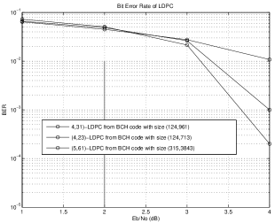
Figure 1: Type I: The error performance of an (4,31) LDPC code with rate $27/31$ and H matrix with size $(124,961)$ based on a BCH code.

VI Conclusion

We introduced two families of regular LDPC codes based on nonprimitive narrow-sense BCH codes and structures of cyclotomic cosets. We gave a systematic method to write every element in the parity check matrix of BCH codes as vector of length $\mu$. We demonstrated that these constructed codes have high rates and a uniform structure that made it easy to compute their dimensions, stopping distance, and bound their minimum distance. Furthermore, one can use standard iterative decoding algorithms to decode these codes. One can easily derive irregular LDPC codes based on these codes and possibly increase performance of the iterative decoding. Also, in future research, these constructed codes can be used to derive quantum LDPC error-correcting codes.

References

- [1] S. A. Aly. A class of quantum LDPC codes constructed from finite geometries. In Proc. 2008 IEEE International Symposium on Information Theory, Toronto, Canada, Submitted 2008. arXiv:quant-ph/0712.4115.
- [2] S. A. Aly and A. Klappenecker. Subsysem code constructions. Phys. Rev. A., on submission. arXiv:quant-ph:0712.4321v2.
- [3] S. A. Aly, A. Klappenecker, and P. K. Sarvepalli. On quantum and classical BCH codes. IEEE Trans. Inform. Theory, 53(3):1183–1188, 2007.
- [4] S. A. Aly, A. Klappenecker, and P. K. Sarvepalli. Primitive quantum BCH codes over finite fields. In Proc. 2006 IEEE International Symposium on Information Theory, pages 1114 – 1118, Seattle, USA, July 2006.
- [5] A. R. Calderbank, E. M. Rains, P. W. Shor, and N. J. A. Sloane. Quantum error correction via codes over GF(4). IEEE Trans. Inform. Theory, 44:1369–1387, 1998.
- [6] M.C. Davey and D.J.C. MacKay. Low density parity check codes over GF(q). IEEE Commun. Lett., 2(6):165–67, 1998.
- [7] C. Di, I.E. Proietti, Telatar, T.J. Richardson, and R. Urbanke. Finite-length analysis of low-density parity check codes on the binary erasure channel. IEEE Trans. Inform. Theory, 48:1570– 1579, June 2000.
- [8] A. M. Evans, Z. W. E. Stephens, J. H. Cole, and L. C. L. Hollenberg. Error correction optimisation in the presence of x/z asymmetry, 2007.
- [9] R.G. Gallager. Low density parity check codes. IRE Trans. Inform. Theory, 8, 1962.
- [10] M. Hagiwara and H. Imai. Quantum quasi-cyclic LDPC codes. Proc. 2007 IEEE International Symposium on Information Theory, 2007. quant-ph 701020v1.
- [11] K. M. Krishnan and P. Shankar. Computing the stopping distance of a tanner graph is NP-hard. IEEE Trans. Inform. Theory, To appear, 2007.
- [12] S. Lin and D.J. Costello. Error Control Coding. Pearson, Prentice Hall, 2004.
- [13] G. Liva, S. Song, Y. Ryan W. Lan, L. Zhang, and S. Lin. Design of LDPC codes: A survey and new results. to appear in J. Comm. Software and Systems, 2006.
- [14] M. G. Luby, M. Mitzenmacher, M. A. Shokrallahi, and D. A. Spielman. Improved low-density parity-check codes using irregular graphs. IEEE Trans. Inform. Theory, 47:585–598, 2001.
- [15] D. J. C. MacKay, G. Mitchison, and P. L. McFadden. Sparse-graph codes for quantum error correction. IEEE Trans. Inform. Theory, 50(10):2315–2330, 2004.
- [16] A. Orlitsky, K. Viswanatham, and J. Zhang. Stopping set distribution of LDPC code ensembles. IEEE Trans. Inform. Theory, 51(3):929–949, March 2005.
- [17] M. Schwartz and A. Vardy. On the stopping distance and the stopping redundancy of codes. IEEE Trans. Inform. Theory, 55(3):922– 932, March 2006.
- [18] S. Song, L. Zeng, S. Lin, and K. Abdel-Ghaffar. Algebraic constructions of nonbinary quasi-cyclic LDPC codes. Proc. 2006 IEEE Intl. Symp. Inform. Theory, pages 83–87, 2006.
- [19] A. M. Steane. Simple quantum error correcting codes. Phys. Rev. Lett., 77:793–797, 1996.
- [20] R.M. Tanner. A recursive approach to low complexity codes. IEEE Trans. Inform. Theory, 27:533–47, 1981.
- [21] R.M. Tanner, D. Sridhara, A. Sridharan, T. Fuja, and D. Costello Jr. LDPC block and convolutional codes based on circulant matricies. IEEE Trans. Inform. Theory, 50(12):2966–2984, December 2004.
- [22] Y. Yi, L. Shaobo, and H. Dawei. Construction of LDPC codes based on narrow-sense primitive BCH codes. Vehicular Technology Conference, 2005, 3:1571 – 1574, 2005.