Quantum theory of electron tunneling into intersubband cavity polariton states

Abstract

Through a non-perturbative quantum theory, we investigate how the quasi-electron excitations of a two-dimensional electron gas are modified by strong coupling to the vacuum field of a microcavity. We show that the electronic dressed states originate from a Fano-like coupling between the bare electron states and the continuum of intersubband cavity polariton excitations. In particular, we calculate the electron spectral function modified by light-matter interactions and its impact on the electronic injection of intersubband cavity polaritons. The domain of validity of the present theoretical results is critically discussed. We show that resonant electron tunneling from a narrow-band injector can selectively excite superradiant states and produce efficient intersubband polariton electroluminescence.

I Introduction

Cavity quantum electrodynamics in the strong coupling regime is presently the subject of many fascinating investigations in several interesting systems, including ultracold atomsColombe , Cooper pair quantum boxes Wallraff and semiconductor nanostructuresHennessy . In the strong coupling regime, the eigenstates of a cavity system are a coherent mixing of photonic and electronic excitations. This occurs when the light-matter interaction, quantified by the so-called vacuum Rabi frequency, is dominant with respect to loss mechanisms for the cavity photon field and for the electronic transition.

Recently, the strong coupling regime has been demonstrated also between a planar microcavity mode and an intersubband transition in a doped semiconductor quantum well. The normal modes of such a system are called intersubband cavity polaritons Dini_PRL ; Aji_APL ; Aji_2006 ; SST ; Ciuti_PRA ; Ciuti_vacuum ; Pere ; Luca_APL ; UltraEx . The active electronic transition is between two conduction subbands, where a dense two-dimensional electron gas populates the lowest one. Large vacuum Rabi frequencies can be achieved thanks to the giant collective dipole associated to the dense electron gas and even an unusual ultra-strong coupling regime can be reachedCiuti_PRA ; Ciuti_vacuum ; Simone_PRL .

Electroluminescence experiments in microcavity-embedded quantum cascade devicesLuca_PRL ; EL_model have recently demonstrated that it is possible to obtain intersubband cavity polariton emission after resonant electrical excitation even at room temperature (and even a lasing mechanism has been proposed Scattering ). A fundamental question to address is how the strong interaction with the microcavity vacuum field modifies the quasi-electron states in the quantum well and how the electron tunneling is affected. In this paper, we present a quantum theory to investigate such fundamental problems. We show that the electronic eigenstates originate from a Fano-like coupling between the bare injected electron and the continuum of cavity polariton modes. Our theory demonstrates that resonant electron tunnelling from a narrow-band injector contact can selectively excite polaritonic states leading to ultraefficient polariton electroluminescence.

The paper is organized as follows: in Sec. II, we introduce the general formalism, by presenting the quantum Hamiltonian, the approximations behind it and by introducing the concept of the electron spectral function in the non-interacting case. In Sec. III we present the calculations leading to the spectrum of the Hamiltonian and to the determination of the electron spectral function in the light-matter interacting case. In Sec. IV we calculate the tunneling coupling and the radiative lifetime of the excited states and present the resulting electroluminescence spectra. Conclusions are drawn in Sec V.

II General formalism

To describe the system to investigate, we consider the following quantum Hamiltonian:

$$H = \sum_{\mathbf{k}}\hbar\omega_{1}(k)c_{1,\mathbf{k}}^{\dagger}c_{1,\mathbf{k}}+\sum_{\mathbf{k}}\hbar\omega_{2}(k)c_{2,\mathbf{k}}^{\dagger}c_{2,\mathbf{k}}+\sum_{\mathbf{q}}\hbar\omega_{c}(q)a_{\mathbf{q}}^{\dagger}a_{\mathbf{q}}$$ (1)

$$+\sum_{\mathbf{k,q}}\hbar\chi(q)a_{\mathbf{q}}c_{1,\mathbf{k}}c_{2,\mathbf{k+q}}^{\dagger}+\sum_{\mathbf{k,q}}\hbar\chi^{*}(q)a_{\mathbf{q}}^{\dagger}c_{2,\mathbf{k+q}}c_{1,\mathbf{k}}^{\dagger}~{},$$

where $\hbar\omega_{1}(k)=\frac{\hbar^{2}\mathbf{k}^{2}}{2m^{\star}}$ and $\hbar\omega_{2}(k)=\hbar\omega_{12}+\frac{\hbar^{2}\mathbf{k^{2}}}{2m^{\star}}$ are the energy dispersions of the two quantum well conduction subbands as a function of the in-plane wavevector $\mathbf{k}$, $m^{\star}$ being the effective mass. The corresponding electron creation operators are $c_{1,\mathbf{k}}^{\dagger}$ and $c_{2,\mathbf{k}}^{\dagger}$. $\omega_{c}(q)$ is the frequency dispersion of the cavity photonic mode and $a_{\mathbf{q}}^{\dagger}$ is the corresponding photon creation operator. Due to the selection rules of intersubband transitions, we omit the photon polarization, which is assumed to be Transverse Magnetic (TM). Being all the interactions spin-conserving, we can omit the electron spin. For simplicity, we consider only a photonic branch, which is quasi-resonant with the intersubband transition, while other cavity modes are supposed to be off-resonance. The interaction between the cavity photon field and the two electronic conduction subbands is quantified by the coupling constant

$$\chi(q)=\sqrt{\frac{\omega_{12}^{2}d_{12}^{2}}{\hbar\epsilon_{0}\epsilon_{r}L_{cav}S\omega_{c}(q)}\frac{q^{2}}{(\pi/L_{cav})^{2}+q^{2}}}~{},$$ (2)

where $c$ is the light speed, $d_{12}$ is the intersubband transition dipole , $\epsilon_{r}$ is the cavity dielectric constant and $S$ is the sample area. Here, we have considered the simple case of a $\lambda/2$-cavity of lenght $L_{cav}$, where $\pi/L_{cav}$ is the cavity photon quantized vector along the growth direction. The geometrical factor $\frac{q^{2}}{(\pi/L_{cav})^{2}+q^{2}}$ is due to the TM-polarization nature of the intersubband transition. Here, for simplicity, we are considering the case of just a single quantum well coupled to the cavity quantum field. Notice that in the Hamiltonian in Eq. (1) the anti-resonant terms of the light-matter interaction have not been included. Therefore, here we can describe the strong coupling for the two subband system, but not all the peculiar features of the ultrastrong coupling regime Ciuti_vacuum ; Ciuti_PRA ; Simone_PRL ; UltraEx .

If one is interested in describing the dynamics of the microcavity under optical excitation, it is possible to use an effective Hopfield Hamiltonian with bosonic operators associated to the intersubband polaritons, which are the elementary optical excitations of the system. If, instead, one is interested in studying microscopically how the electronic injection into to such a microcavity system is modified by non-perturbative light-matter excitation, it is necessary to work with the full fermionic Hamiltonian in Eq. (1). In fact, electrical excitation occurs through injection of (fermionic) carriers: the dynamics must include the (bosonic) optical excitations and the electronic (fermionic) excitations at the same level. As well known in the theory of quantum transportDatta , if we wish to study the tunneling injection of one electron at low temperature, we have to determine the electron spectral function, defined as:

$$A^{+}_{j}(\mathbf{k},\omega)=\sum_{\zeta}\lvert\langle\zeta|c^{\dagger}_{j,\mathbf{k}}|F_{N}\rangle\lvert^{2}\delta(\omega-\omega_{\zeta})~{},$$ (3)

where $|F_{N}\rangle$ is the N-electron Fermi sea ground state times the vacuum state for the cavity photon field and $j=1,2$ is the conduction subband index. The index $\zeta$ labels the excited (N+1)-electron eigenstates and $\hbar\omega_{\zeta}$ are the corresponding eigenenergies. Note that even if in the present paper we consider the case of zero temperature, the theory can be applied as far as $K_{B}T$ is much smaller than the Fermi energy of the two-dimensional electron gas.

As apparent from Eq. (3), the electron spectral function is the density of quasi-electron states, weighted by the overlap with the bare electron state $c^{\dagger}_{j,\mathbf{k}}|F_{N}\rangle$. In other words, it is the many-body equivalent of the single electron density of states. This is the key quantity affecting the electron tunneling and can be non-trivially modified by interactions like in the case of superconductors. For a non-interacting electron gas, $c^{\dagger}_{1,\mathbf{k}}|F_{N}\rangle$ and $c^{\dagger}_{2,\mathbf{k}}|F_{N}\rangle$ are eigenstates of the Hamiltonian and thus all the other eigenstates are orthogonal to them. Therefore the non-interacting spectral functions are

$$A^{+}_{1}(\mathbf{k},\omega) = \delta(\omega-\omega_{1}(k))\theta(k-k_{F}),$$ (4)

$$A^{+}_{2}(\mathbf{k},\omega) = \delta(\omega-\omega_{2}(k)),$$ (5)

where $k_{F}$ is the Fermi wavevector. $\theta(x)$ is the Heaviside function and its presence is due to Pauli blocking: $c^{\dagger}_{1,\mathbf{k}}|F_{N}\rangle=0$ for $k<k_{F}$.

III Spectral function with light-matter interactions

As seen in the previous section, in the non-interacting case, the electron spectral function is just a Dirac delta. Physically, this means that an electron with wavevector $\mathbf{k}$ can be injected in the subband $j=1,2$ only with an energy equal to the bare electron energy $\hbar\omega_{j}(k)$ and that such excitation has an infinite lifetime. By contrast, interactions can profoundly modify the nature of electron excitations and therefore produce qualitative and quantitative changes of the electron spectral functions. In the case of a weakly interacting electron gas, the spectral function has a broadened ”quasi-electron” peak: the spectral broadening is due to the finite lifetime of the electronic excitation. In the case of a strongly interacting electron gas (like in the case of superconductors) the electron spectral function can be qualitatively different from the non-interacting gas. Here, we are interested in how the nature of the quasi-electron excitations is modified by the strong coupling to the vacuum field of a microcavity. In particular, we assume that the light-matter interaction is the strongest one. We will provide here a nonperturbative theory to determine the dressed electronic excitations in such a strong coupling limit and their corresponding spectral function. All other residual interactions will be treated as perturbations. The consistency and limit of validity of such a scheme will be discussed in the next section, where the theoretical results are applied.

In the interacting case, it is easy to verify that $c^{\dagger}_{1,\mathbf{k}}|F_{N}\rangle$ is still an eigenvector of the Hamiltonian in Eq. (1) and thus the first subband spectral function $A_{1}^{+}(\mathbf{k},\omega)$ is still given by Eq. (4). Instead for the electrons in the second subband we have to distinguish between two cases: $\mathbf{k}$ well inside or outside the Fermi sea. In the first case, an electron in the second subband can not emit a photon because all the final states in the first subband are occupied (Pauli blocking), hence the spectral function will be given by the unperturbed one (Eq. (5)). Well outside the Fermi sea, an injected electron can emit and the spectral function will be modified by the light-matter interaction. A smooth transition between the two cases will take place for $\lvert k-k_{F}\lvert$ of the order of the resonant cavity photon wave-vector $q_{res}$, where $\omega_{c}(q_{res})=\omega_{12}$. Being the ratio $q_{res}/k_{F}$ typically very small, of the order of $10^{-2}$ (see Ref. [Aji_excited, ]), we can safely consider an abrupt transition at the Fermi edge.

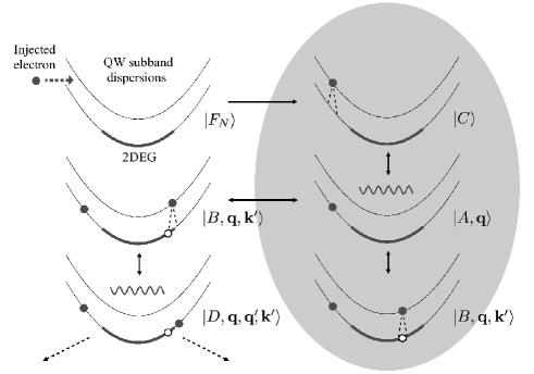
Figure 1: Sketch of the dynamical coupling between quantum states in a microcavity-embedded quantum well (QW) containing a two-dimensional electron gas (2DEG). In the ground state, the first subband is doped with a dense 2DEG (bold lines at the bottom of the dispersions). Black dots represent bare electrons, while white dots denote holes in the 2DEG. The dashed cones depicts the possible final states for an electron radiatively relaxing from the second to the first subband by emission of a cavity photon. The ground state with $N$ electrons is the standard Fermi sea $|F_{N}\rangle$. The injection (e.g., through electron tunneling) of an additional electron in the second subband creates the state $|C\rangle=c^{\dagger}_{2,\mathbf{k}}|F_{N}\rangle$, which, in presence of light-matter interaction, is not an eigenstate. Spontaneous emission of a cavity photon couples the $|C\rangle$ state to the states $|A,\mathbf{q}\rangle=a^{\dagger}_{\mathbf{q}}c^{\dagger}_{1,\mathbf{k-q}}|F_{N}\rangle$. Reabsorption of the emitted cavity photon can couple back to the $|C\rangle$ state or to the states $|B,\mathbf{q,k^{\prime}}\rangle=c^{\dagger}_{2,\mathbf{k^{\prime}+q}}c_{1,\mathbf{k^{\prime}}}c^{\dagger}_{1,\mathbf{k-q}}|F_{N}\rangle$. Spontaneous emission couples the $|B\rangle$ states back to $|A\rangle$ states or to states of the form $|D,\mathbf{q,q^{\prime},k^{\prime}}\rangle=a^{\dagger}_{\mathbf{q^{\prime}}}c_{1,\mathbf{k^{\prime}+q-q^{\prime}}}^{\dagger}c_{1,\mathbf{k^{\prime}}}c^{\dagger}_{1,\mathbf{k-q}}|F_{N}\rangle$. Being the relevant cavity photon wavevectors very small compared to the Fermi wavevector, spontanous emission can occur only on narrow emission cone in momentum space. Due to the small probability of photon absorption by electrons on the border the Fermi sea, we can neglect $|D\rangle$ states and assume that the system always jumps from $|B\rangle$ states to $|A\rangle$ states. Thus the relevant dynamics takes place only between the states in the shaded region. We can thus neglect the other marginal states while diagonalizing the light-matter Hamiltonian.

For evaluating $A_{2}^{+}(\mathbf{k},\omega)$ for $k>k_{F}$ we need to find all the (N+1)-electron eigenstates that have a nonzero overlap with $c^{\dagger}_{2,\mathbf{k}}|F_{N}\rangle$. In order to do this we notice that the Hamiltonian in Eq. (1) commutes with the number of total fermions

$$\hat{N}_{F}=\sum_{j=1,2}\sum_{\mathbf{k}}c_{j,\mathbf{k}}^{\dagger}c_{j,\mathbf{k}},$$

the total in plane wave-vector operator

$$\hat{\mathbf{K}}=\sum_{j=1,2}\sum_{\mathbf{k}}\mathbf{k}~{}c_{j,\mathbf{k}}^{\dagger}c_{j,\mathbf{k}}+\sum_{\mathbf{q}}\mathbf{q}a^{\dagger}_{\mathbf{q}}a_{\mathbf{q}},$$

and the excitation number operator

$$\hat{Q}=\sum_{\mathbf{k}}c_{2,\mathbf{k}}^{\dagger}c_{2,\mathbf{k}}+\sum_{\mathbf{q}}a_{\mathbf{q}}^{\dagger}a_{\mathbf{q}}.$$

Hence the eigenstates $|\zeta\rangle$ of $H$ can be also labeled by the corresponding eigenvalues $N_{\zeta},\mathbf{K_{\zeta}}$ and $Q_{\zeta}$. We will thus identify an eigenstate of $H$ in the subspace $(\hat{N_{F}}=N,\mathbf{\hat{K}=\mathbf{K}},\hat{Q}=Q)$ as $|N,\mathbf{K},Q,\zeta\rangle$, where the index $\zeta$ now runs over all the eigenstates of the subspace The states obtained by applying electron creation or destruction operators on the eigenstates $|{N,\mathbf{K},Q,\zeta}\rangle$ are still eigenstates of $\hat{N}_{F}$, $\hat{\mathbf{K}}$ and $\hat{\mathbf{Q}}$. The state $c_{1,\mathbf{k}}^{\dagger}|{N,\mathbf{K},Q,\zeta}\rangle$ is in the subspace labeled by the quantum numbers $(N+1,\mathbf{K+k},Q)$; $c_{1,\mathbf{k}}|{N,\mathbf{K},Q,\zeta}\rangle$ in $(N-1,\mathbf{K-k},Q)$; $c_{2,\mathbf{k}}^{\dagger}|{N,\mathbf{K},Q,\zeta}\rangle$ in $(N+1,\mathbf{K+k},Q+1)$; $c_{2,\mathbf{k}}|{N,\mathbf{K},Q,\zeta}\rangle$ in $(N-1,\mathbf{K-k},Q-1)$.

Having $|F_{N}\rangle$ quantum numbers (N,0,0) the state $c_{2,\mathbf{k}}^{\dagger}|F\rangle$ is thus in the subspace labeled by the quantum numbers $(N+1,\mathbf{k},1)$. We can limit ourselves to diagonalize $H$ in this subspace, which is spanned by vectors of the form: (i) $c^{\dagger}_{2,\mathbf{k}_{0}}\prod_{j=1}^{N}c^{\dagger}_{1,\mathbf{k}_{j}}|0\rangle$, where $|0\rangle$ is the empty conduction band state and $\sum_{j=1}^{N}\mathbf{k}_{j}=\mathbf{k}-\mathbf{k}_{0}$; (ii) $a^{\dagger}_{\mathbf{q}_{0}}\prod_{j=1}^{N+1}c^{\dagger}_{1,\mathbf{k}_{j}}|0\rangle$ with $\sum_{j=1}^{N+1}\mathbf{k}_{j}=\mathbf{k}-\mathbf{q}_{0}$. For a large number of electrons, the exact diagonalization of the Hamiltonian in this subspace is an unmanageable task. Here, we show that by a judicious approximation, we can considerably simplify the diagonalization problem, keeping the relevant non-perturbative physics. Namely, we claim that the elements of the ($N+1,\mathbf{k},1$) subspace can be well approximated by vectors of the form

$$|N+1,\mathbf{k},1,\zeta\rangle=\left\{\mu_{\zeta}~{}c^{\dagger}_{2,\mathbf{k}}+\sum_{\mathbf{q}}\left[\alpha_{\zeta}(\mathbf{q})~{}a^{\dagger}_{\mathbf{q}}c^{\dagger}_{1,\mathbf{k-q}}+\sum_{\mathbf{\lvert k^{\prime}\lvert}<k_{F}}\beta_{\zeta}~{}(\mathbf{q,k^{\prime}})c^{\dagger}_{2,\mathbf{k^{\prime}+q}}c_{1,\mathbf{k^{\prime}}}c^{\dagger}_{1,\mathbf{k-q}}\right]\right\}|F_{N}\rangle~{}.$$ (6)

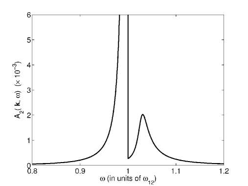
Figure 2: Electron spectral function $A^{+}_{2}(\mathbf{k},\omega)$ for the second subband , for all $k>k_{F}$. The spectral function, defined in Eq. (3), is the density of quasi-electron states, weighted by the overlap with the bare electron state.The integral of the spectral function over the frequency $\omega$ is by construction equal to one. Coupling parameter: $\Omega_{R}(q_{res})=\lvert\chi(q_{res})\lvert\sqrt{N}=0.1\omega_{12}$.

To understand the origin of our approximation, let us consider the time evolution picture sketched in Fig. 1. Suppose that initially the system is in its ground state $|F_{N}\rangle$. After injection of one bare electron, the state of the system is

$$|C\rangle=c^{\dagger}_{2,\mathbf{k}}|F_{N}\rangle.$$

If $\mathbf{k}$ is well inside the Fermi sphere, as we said before, it is Pauli blocked and can not radiatively relax into the first subband. Instead, when $k>k_{F}$, the injected electron can radiatively decay, emitting a photon and falling into the first subband. After the first emission the state will have the form

$$|A,\mathbf{q}\rangle=a^{\dagger}_{\mathbf{q}}c^{\dagger}_{1,\mathbf{k-q}}|F_{N}\rangle.$$

If the cavity system is closed and only the light-matter interaction is considered, the emitted photon will be eventually reabsorbed. The system can evolve back to the state $|C\rangle$ or into one vector of the form

$$|B,\mathbf{q,k^{\prime}}\rangle=c^{\dagger}_{2,\mathbf{k^{\prime}+q}}c_{1,\mathbf{k^{\prime}}}c^{\dagger}_{1,\mathbf{k-q}}|F_{N}\rangle.$$

If $\mathbf{k^{\prime}}$ is well inside the Fermi sea, when the second subband electron decays, the only avaiable final state in the first subband will be the one with wavevector $\mathbf{k^{\prime}}$, that is the system will go back to state $|A,\mathbf{q}\rangle$. If $\mathbf{k^{\prime}}$ is on the border of the Fermi sea, on the contrary, the system can evolve into a state of the form $|D,\mathbf{q,q^{\prime},k^{\prime}}\rangle=a^{\dagger}_{\mathbf{q^{\prime}}}c_{1,\mathbf{k^{\prime}+q-q^{\prime}}}^{\dagger}c_{1,\mathbf{k^{\prime}}}c^{\dagger}_{1,\mathbf{k-q}}|F_{N}\rangle$. The probability of ending in any of the $|D,\mathbf{q,q^{\prime},k^{\prime}}\rangle$ states is negligible. In fact, the probability for $\mathbf{k^{\prime}}$ to be near enough to the border of the Fermi sea for allowing an emission to electronic states with $k>k_{F}$ is proportional to the ratio $q_{res}/k_{F}\ll 1$. Hence, the diagonalization problem can be simplified and we can thus look for vectors of the form shown in Eq. (6).

In such a subspace, spanned by $\{|C\rangle,|A,\mathbf{q}\rangle,|B,\mathbf{q,k^{\prime}}\rangle,|B,\mathbf{q,k^{\prime\prime}}\rangle,\dots,|A,\mathbf{q^{\prime}}\rangle,|B,\mathbf{q^{\prime},k^{\prime}}\rangle,|B,\mathbf{q^{\prime},k^{\prime\prime}}\rangle,\dots\}$, $H$ has the following matrix representation:

$${\mathcal{H}}_{N+1,\mathbf{k},1}=\hbar\left(\begin{array}[]{ccccc}\omega_{2}(k)&v(q)&v(q^{\prime})&v(q^{\prime\prime})&\cdots\\ v(q)^{T}&M(\mathbf{q})&0&0&\cdots\\ v(q^{\prime})^{T}&0&M(\mathbf{q^{\prime}})&0&\cdots\\ v(q^{\prime\prime})^{T}&0&0&M(\mathbf{q^{\prime\prime}})&\ddots\\ \vdots&\vdots&\vdots&\ddots&\ddots\\ \end{array}\right)$$

where $M(\mathbf{q})$ is the Hamiltonian matrix block in the subspace spanned by $\{|A,\mathbf{q}\rangle,|B,\mathbf{q,k^{\prime}}\rangle,|B,\mathbf{q,k^{\prime\prime}}\rangle,\dots\}$, that effectively describes the system in presence of one photon with a well defined wavevector $\mathbf{q}$

$$M(\mathbf{q})=\left(\begin{array}[]{cccc}\omega_{c}(q)+\omega_{1}(|\mathbf{k}-\mathbf{q}|))&\chi^{*}(q)&\chi^{*}(q)&\cdots\\ \chi(q)&\omega_{2}(|\mathbf{k^{\prime}}+\mathbf{q}|)-\omega_{1}(k^{\prime})+\omega_{1}(|\mathbf{k}-\mathbf{q}|)&0&\cdots\\ \chi(q)&0&\omega_{2}(|\mathbf{k^{\prime\prime}}+\mathbf{q}|)-\omega_{1}(k^{\prime\prime})+\omega_{1}(|\mathbf{k}-\mathbf{q}|)&\ddots\\ \vdots&\vdots&\ddots&\ddots\\ \end{array}\right),$$

where $v(q)=[\chi(q),0,0,\dots]$. Since the typical wavevector $q$ of the resonantly coupled cavity photon mode is much smaller than $k_{F}$, we can perform the standard approximation $\omega_{2}(|\mathbf{k^{\prime}}+\mathbf{q}|)-\omega_{1}(k^{\prime})\simeq\omega_{2}(k^{\prime})-\omega_{1}(k^{\prime})=\omega_{12}$. This way, we can exactly diagonalize each of the $M(\mathbf{q})$ blocks. As expected from the theory of optically excited polaritons Ciuti_vacuum , by diagonalizing the matrix $M(\mathbf{q})$ we find two bright electronic states (i.e., with a photonic mixing component)

$$|\pm,\mathbf{q}\rangle = \frac{(\omega_{\pm}(q)-\omega_{12})|A,\mathbf{q}\rangle+\chi(q)\sum_{\mathbf{k}}|B,\mathbf{q,k}\rangle}{\sqrt{\left(\omega_{\pm}(q)-\omega_{12}\right)^{2}+\lvert\chi(q)\lvert^{2}N}}~{},$$ (7)

with energies $\hbar\omega_{1}(k)+\hbar\omega_{\pm}(q)$, where

$$\omega_{\pm}(q)=\frac{\omega_{c}(q)+\omega_{12}}{2}\pm\sqrt{\left(\frac{\omega_{c}(q)-\omega_{12}}{2}\right)^{2}+N\lvert\chi(q)\lvert^{2}}~{}.$$ (8)

Note that $\hbar\omega_{\pm}(q)$ are the energies of the two branches of intersubband cavity polaritons Ciuti_vacuum .

The other orthogonal states are dark (no photonic component), with eigenvalues $\omega_{2}(k)=\omega_{1}(k)+\omega_{12}$ and eigenvectors

$$|l,\mathbf{q}\rangle = \frac{\sum_{\mathbf{k}}\beta_{l}(\mathbf{q,k})|B,\mathbf{q,k}\rangle}{\sqrt{N}}$$ (9)

where the $\beta_{l}(\mathbf{q,k})$ are such that $\sum_{\mathbf{k}}\beta_{l}(\mathbf{q,k})=0$ and $\sum_{\mathbf{k}}\beta_{l}(\mathbf{q,k})\beta_{l^{\prime}}^{*}(\mathbf{q,k})=\delta_{l,l^{\prime}}$.

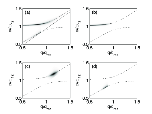
Figure 3: Extracavity electroluminescence spectra $N_{ph}(\mathbf{q},\omega)$. Panel (a): the case of a broadband electrical injector (bandwidth equal to $\omega_{12}$, centered at $\omega=\omega_{12}$). The other panels show the results for a narrow-band injector (width $0.05\omega_{12}$) centered respectively at $\omega=\omega_{12}$ (b), $1.2\omega_{12}$ (c) and $0.8\omega_{12}(d)$. The non-radiative relaxation rate $1/\tau_{nr,\mathbf{k},\zeta}$ has been taken equal to $0.005\omega_{12}$. In all panels, the dashed-dotted lines are the frequency dispersions $\omega_{\pm}(q)$ of the two cavity polariton branches. In the first panel the solid line represents the edge of the light cone Aji_excited .

Since $\langle l,\mathbf{q}|H~{}c_{2,\mathbf{k}}^{\dagger}|F_{N}\rangle=0$, the dark states $|l,\mathbf{q}\rangle$ are also eigenstates of the matrix ${\mathcal{H}}_{N+1,\mathbf{k},1}$ and do not contribute to the electron spectral function, because they have zero overlap with the state $|C\rangle=c_{2,\mathbf{k}}^{\dagger}|F_{N}\rangle=0$. In contrast, this is not the case for the bright eigenstates of each block $M({\mathbf{q}})$, as we find:

$$\langle\pm,\mathbf{q}|H~{}c_{2,\mathbf{k}}^{\dagger}|F_{N}\rangle=\frac{\chi(q)^{*}(\omega_{\pm}(q)-\omega_{12})}{\sqrt{(\omega_{\pm}(q)-\omega_{12})^{2}+\lvert\chi(q)\lvert^{2}N}}=J_{\pm}^{*}(q)~{}.$$ (10)

Therefore, the representation of $H$ in the subspace $\{|C\rangle,|+,\mathbf{q}\rangle,|-,\mathbf{q}\rangle,|+,\mathbf{q^{\prime}}\rangle,|-,\mathbf{q^{\prime}}\rangle,\dots\}$ reads

$${\mathcal{H}^{\prime}}_{N+1,\mathbf{k},1}=\hbar\left(\begin{array}[]{cccccc}\omega_{1}(k)+\omega_{12}&J_{+}^{*}(q)&J_{-}^{*}(q)&J_{+}^{*}(q^{\prime})&J_{-}^{*}(q^{\prime})&\cdots\\ J_{+}(q)&\omega_{1}(k)+\omega_{+}(q)&0&0&0&\cdots\\ J_{-}(q)&0&\omega_{1}(k)+\omega_{-}(q)&0&0&\cdots\\ J_{+}(q^{\prime})&0&0&\omega_{1}(k)+\omega_{+}(q^{\prime})&0&\cdots\\ J_{-}(q^{\prime})&0&0&0&\omega_{1}(k)+\omega_{-}(q^{\prime})&\cdots\\ \vdots&\vdots&\vdots&\vdots&\vdots&\ddots\\ \end{array}\right).$$

Hence, here we have demonstrated that the bare electron state $c_{2,\mathbf{k}}^{\dagger}|F_{N}\rangle$ is coupled to the continuum of the polariton modes with all the different wavevectors q. Since the polariton frequencies $\omega_{\pm}$ and the coupling $J_{\pm}$ depend only on the modulus of q, we can further simplify the diagonalization problem by introducing the ’annular’ bright states

$$|\pm,q\rangle=\frac{1}{\sqrt{Lq}}\sum_{\lvert\mathbf{q}\lvert=q}|\pm,\mathbf{q}\rangle~{},$$ (11)

where $L=\sqrt{S}$ and $2\pi/L$ is the linear density of modes in reciprocal space. All annular states are coupled to $|C\rangle$. Instead, all the orthogonal linear combinations of $|\pm,\mathbf{q}\rangle$ (with $\lvert\mathbf{q}\lvert=q$) are uncoupled and therefore do not contribute to the electron spectral function. The matrix representation of $H$ in the subspace $\{|C\rangle,|+,q\rangle,|-,q\rangle,|+,q^{\prime}\rangle,|-,q^{\prime}\rangle,\dots\}$ reads

$${\mathcal{H}^{\prime\prime}}_{N+1,\mathbf{k},1}=\hbar\left(\begin{array}[]{cccccc}\omega_{1}(k)+\omega_{12}&J_{+}^{*}(q)\sqrt{Lq}&J_{-}^{*}(q)\sqrt{Lq}&J_{+}^{*}(q^{\prime})\sqrt{Lq^{\prime}}&J_{-}^{*}(q^{\prime})\sqrt{Lq^{\prime}}&\cdots\\ J_{+}(q)\sqrt{Lq}&\omega_{1}(k)+\omega_{+}(q)&0&0&0&\cdots\\ J_{-}(q)\sqrt{Lq}&0&\omega_{1}(k)+\omega_{-}(q)&0&0&\cdots\\ J_{+}(q^{\prime})\sqrt{Lq^{\prime}}&0&0&\omega_{1}(k)+\omega_{+}(q^{\prime})&0&\cdots\\ J_{-}(q^{\prime})\sqrt{Lq^{\prime}}&0&0&0&\omega_{1}(k)+\omega_{-}(q^{\prime})&\ddots\\ \vdots&\vdots&\vdots&\vdots&\ddots&\ddots\end{array}\right)$$ (12)

Hence, in the subspace ($N+1,\mathbf{k},1$), we have found that eigenstates of $H$ with a finite overlap with the bare electron have the form

$$|N+1,\mathbf{k},1,\zeta\rangle=\mu_{\zeta}~{}c^{\dagger}_{2\,\mathbf{k}}|F_{N}\rangle+\sum_{q,\sigma=\pm}\lambda_{\zeta,\sigma,q}|\sigma,q\rangle~{}.$$ (13)

The coefficients $\mu_{\zeta}$ and $\lambda_{\zeta,\sigma,q}$ as well as the corresponding energy eigenvalues $\hbar\omega_{\zeta}$ can be calculated though a numerical diagonalization of the matrix in Eq. (12). In conclusion, the spectral function of the second subband reads

$$A^{+}_{2}(\mathbf{k},\omega)=\sum_{\zeta}\lvert\mu_{\zeta}\lvert^{2}\delta(\omega-\omega_{\zeta})\theta(k-k_{F})+\delta(\omega-\omega_{2}(k))\theta(k_{F}-k).$$ (14)

In Fig. 2, we show numerical results using a vacuum Rabi frequency $\Omega_{R}(q_{res})=\lvert\chi(q_{res})\rvert\sqrt{N}=0.1\omega_{12}$. As it appears from Eq. (14), the broadening of the spectral function is intrinsic, being associated to the continuum spectrum of frequencies $\omega_{\zeta}$ corresponding to the dressed electronic states and given by the eigenvalues of the infinite matrix in Eq. (12). At each frequency $\omega_{\zeta}$, the magnitude of the spectral function is given by the spectral weight $\lvert\mu_{\zeta}\lvert^{2}$, depending on the overlap between the dressed state $|N+1,\mathbf{k},1,\zeta\rangle$ and the bare electron state $|C\rangle=c^{\dagger}_{2,\mathbf{k}}|F_{N}\rangle$. As shown in Eq. (12), the electronic eigenstates of the system are given by the Fano-like coupling between the bare electron state and the continuum of cavity polariton excitations. Indeed, the pronounced dip around $\omega=\omega_{12}$ in the spectral function is a quantum interference feature, typical of a Fano resonanceFano .

As we said before the sharp transition in Eq. 14 between $k>k_{F}$ and $k<k_{F}$ is only a consequence of the approximations we made of neglecting the border of the Fermi sea and the effect of the temperature. In a real case both effects will tend to smooth the transition, the first on an energy scale of the order of $\frac{\hbar^{2}k_{F}q_{res}}{m^{*}}$ and the second on an energy scale of $K_{B}T$.

IV Tunneling coupling, losses and electroluminescence

The states $|N+1,\mathbf{k},1,\zeta\rangle$ have been obtained by diagonalizing the Hamiltonian (1), which takes into account only the coupling between the two-subband electronic system and the microcavity photon quantum field. If, as we have assumed, the light-matter interaction is the strongest one, all other residual couplings can be treated perturbatively. These residual interactions include the coupling to the extracavity fields, the interaction with contacts, phonon and impurity scattering as well as Coulomb electron-electron interactionsCoulomb .

The states $|N+1,\mathbf{k},1,\zeta\rangle$ can be excited for example by resonant electron tunneling from a bulk injector or an injection miniband. If $V^{tc}_{\mathbf{k}}$ is the tunneling coupling matrix element between the state $|F\rangle$ and $c^{\dagger}_{2,\mathbf{k}}|F\rangle$ induced by the coupling with the injector we have, using the Fermi golden rule, the following injection rate:

$$\Gamma_{inj}(\mathbf{k},\zeta)=\frac{2\pi}{\hbar}\lvert\mu_{\zeta}\lvert^{2}\lvert V^{tc}_{\mathbf{k}}\lvert^{2}\rho_{inj}(\omega_{\zeta})n_{F}(\omega_{\zeta}),$$ (15)

where $\rho_{inj}(\omega)$ is the density of electronic states inside the contact and $n_{f}(\omega)$ its Fermi distribution. $\rho_{inj}(\omega)n_{f}(\omega)$ determines the spectral shape of the injector. $\mu_{\zeta}$ comes from Eq. (14) and represents the electron spectral weight.

It is worthwhile to notice that the formula in Eq. 15 is quite independent from the model of injector considered. All the relevant informations are contained in the coupling strenght $V^{tc}_{\mathbf{k}}$ and the spectral shape $\rho_{inj}(\omega)n_{f}(\omega)$. Any form of scattering, including in-plane wavevector non-conserving interactions or non-resonant injection, will simply give a different (and possibly broadened) injector spectral shape.

The finite transmission of the cavity mirrors is responsible for a finite lifetime for the cavity photons and consequently for the dressed states $|N+1,\mathbf{k},1,\zeta\rangle$. By using the Fermi golden rule and a quasi-mode coupling to the extracavity field, we find that the radiative lifetime $\tau_{r,\mathbf{k},\zeta}$ reads:

$$\frac{1}{\tau_{r,\mathbf{k},\zeta}} = \frac{2\pi}{\hbar}\sum_{\mathbf{q},q_{z}}|\alpha_{\zeta}(\mathbf{q})\lvert^{2}\lvert V^{qm}_{\mathbf{q},q_{z}}\lvert^{2}\delta(\hbar\omega_{\zeta}-\hbar\omega_{\mathbf{q},q_{z}})\theta(k-k_{F}),$$

where $V^{qm}_{\mathbf{q},q_{z}}$ is the quasi-mode coupling matrix element, $\omega_{\mathbf{q},q_{z}}$ the extracavity photon frequency and $\alpha_{\zeta}(\mathbf{q})=\langle A,\mathbf{q}|N+1,\mathbf{k},1,\zeta\rangle$ as defined in Eq. (6). Having calculated the tunneling injection rate and the radiative lifetime for the different states, we are able to evaluate the electroluminescence spectra. It is convenient to introduce the normalized photon emission distribution corresponding to each eigenstate $|N+1,\mathbf{k},1,\zeta\rangle$, namely

$$L(\mathbf{q},\zeta) = \mathcal{N}\sum_{q_{z}}\lvert\alpha_{\zeta}(\mathbf{q})\lvert^{2}\lvert V^{qm}_{\mathbf{q},q_{z}}\lvert^{2}\delta(\hbar\omega_{\zeta}-\hbar\omega_{\mathbf{q},q_{z}}),$$ (16)

where the normalization $\mathcal{N}$ is fixed by imposing $\sum_{\mathbf{q}}L(\mathbf{q},\zeta)=1$. The number of photons with in-plane wave-vector $\mathbf{q}$ and frequency $\omega$ emitted per unit time is

$$N_{ph}(\mathbf{q},\omega)=\frac{1}{\pi}\sum_{\mathbf{k},\zeta}\Gamma_{inj}(\mathbf{k},\zeta)L(\mathbf{q},\zeta)\frac{1/\tau_{r,\mathbf{k},\zeta}}{(\omega-\omega_{\zeta})^{2}+(1/\tau_{r,\mathbf{k},\zeta}+1/\tau_{nr,\mathbf{k},\zeta})^{2}}~{},$$ (17)

where the last factor accounts for the Lorentzian broadening due to radiative and non-radiative processes. $\tau_{nr,\mathbf{k},\zeta}$ is the non-radiative lifetime of the electronic excitations and $\Gamma_{inj}(\mathbf{k},\zeta)$ is given by Eq. (15). Fig. 3 reports representative electroluminescence spectra in the case of a broadband (panel a) and narrowband (panel b,c,d) injector. In the broadband case, the emission is resonant at the intersubband cavity polariton frequencies (dashed lines) and it is significant in a wide range of in-plane wavectorsEL_model . In contrast, in the case of narrowband electrical injector our theory shows that the photon in-plane momentum and the energy of the cavity polariton emission can be selected by the resonant electron tunneling process, in agreement with what suggested by recent experiments Luca_PRL .

In free-space, the quantum efficiency of electroluminescent devices based on intersubband transitions is poor ($\approx 10^{-5}$ in the mid-infrared) due to the slow radiative recombination of long wavelength transitions. In the microcavity case, the efficiency of the emission from an excited state $|N+1,\mathbf{k},1,\zeta\rangle$ is given by $(1+\tau_{r,\mathbf{k},\zeta}/\tau_{nr,\mathbf{k},\zeta})^{-1}$. Being $1/\tau_{nr,\mathbf{k},\zeta}$ essentially proportional to the matter component of the excitation and $1/\tau_{r,\mathbf{k},\zeta}$ to its photonic fraction, we have found that it is possible to obtain a quantum efficiency approaching unity by selectively injecting electrons into dressed states with a high photonic fraction. In particular, this is achievable by avoiding injection resonant with the central peak of the electron spectral function in Fig.2, which corresponds to states with strong overlap with the bare electron state.

In the present theory, we have not considered the role of electronic disorder, which is known to break the in-plane translational invariance. However, in the limit of large vacuum Rabi energies (i.e., significantly larger than the energy scale of the disorder potential), the inhomogenous broadening is expected to have a perturbative role.

Let us point out clearly that in order to achieve a high quantum efficiency, it is necessary to have a considerably narrow spectral width for the injector, on the order of a small fraction ($10^{-2}$) of the intersubband transition energy $\hbar\omega_{12}$. This is essential in order to be able to inject electrons selectively into the superradiant states, while avoiding both the peak associated to the dark excitations at the bare electron energy and the states with $k<k_{F}$ that can not radiatively decay. In the experiments in Ref. Luca_PRL, , the spectral width of the injector (a heavily doped superlattice) is comparable to the polariton vacuum Rabi frequency and hence such selective excitations of the superradiant states cannot be reached. In order to have an injector with narrower spectral width, several electronic designs could be implemented. For example, one can grow a ”filter” quantum well between the superlattice injector and the active quantum well: resonant electron tunneling through the intermediate quantum well can significantly enhance the resonant character of the excitation. Moreover, for a given injector, improved microcavity samples with larger vacuum Rabi frequency would allow the system a more resonant excitation of the superradiant electronic states.

V Conclusions

In conclusion, we have determined in a non-perturbative way the quasi-electron states in a microcavity-embedded two-dimensional electron gas. Such states originate from a Fano-like coupling between the bare electron state and the continuum of cavity polariton excitations. We have proven that these states can be selectively excited by resonant electron tunneling and that the use of narrow-band injector may give rise to efficient intersubband polariton electroluminescence. Our theoretical work shows that the strong coupling to the vacuum electromagnetic field can modify significantly the fundamental electron injection processes.

VI Acknowledgements

qWe thanks Iacopo Carusotto, Raffaele Colombelli, Alberto Santagostino, Luca Sapienza, Carlo Sirtori, Yanko Todorov and Angela Vasanelli for discussions.

References

- (1) Y. Colombe, T. Steinmetz, G. Dubois, L. Linke, D. Hunger, and J. Reichel, Nature 450, 272-276 (2007).
- (2) A. Wallraff, D. I. Schuster, A. Blais, L. Frunzio, R.-S. Huang, J. Majer, S. Kumar, S. M. Girvin and R. J. Schoelkopf, Nature 431, 162 (2004).
- (3) K. Hennessy, A. Badolato, M. Winger, D. Gerace, M. Atature, S. Gulde, S. Falt, E. L. Hu, and A. Imamoglu, Nature 445, 896 (2007).
- (4) D. Dini, R. Kohler, A. Tredicucci, G. Biasiol, and L. Sorba, Phys. Rev. Lett. 90, 116401 (2003).
- (5) A. A. Anappara, A. Tredicucci, G. Biasiol, L. Sorba, Appl. Phys. Lett. 87, 051105 (2005).
- (6) A. A. Anappara, A. Tredicucci, F. Beltram, G. Biasiol, L. Sorba,Appl. Phys. Lett. 89, 171109 (2006).
- (7) R. Colombelli, C. Ciuti, Y. Chassagneux, C. Sirtori, Semicond. Sci. Technol. 20, 985 (2005).
- (8) A. A. Anappara, S. De Liberato, A. Tredicucci, C. Ciuti, G. Biasiol, L. Sorba, F. Beltram, arXiv:0808.3720.
- (9) C. Ciuti, G. Bastard, I. Carusotto, Phys. Rev. B 72, 115303 (2005).
- (10) C. Ciuti, I. Carusotto, Phys. Rev. A 74, 033811 (2006).
- (11) M. F. Pereira, Phys. Rev. B 75, 195301 (2007).
- (12) L. Sapienza, A. Vasanelli, C. Ciuti, C. Manquest, C. Sirtori, R. Colombelli, and U. Gennser, Appl. Phys. Lett. 90, 201101 (2007).
- (13) S. De Liberato, C. Ciuti, I. Carusotto, Phys. Rev. Lett. 98, 103602 (2007).
- (14) L. Sapienza, A. Vasanelli, R. Colombelli, C. Ciuti, Y.Chassagneux, C. Manquest, U. Gennser, C. Sirtori , Phys. Rev. Lett., 100, 136806 (2008).
- (15) S. De Liberato and C. Ciuti, arXiv:0806.1691.
- (16) S. De Liberato and C. Ciuti, Phys. Rev. B, 77, 155321 (2008)
- (17) S. Datta, Quantum Transport: Atom to Transistor (Cambridge University Press 2005).
- (18) A. A. Anappara, A. Tredicucci, F. Beltram, G. Biasiol, L. Sorba, S. De Liberato, C. Ciuti, Appl. Phys. Lett. 91, 231118 (2007)
- (19) U. Fano, Phys. Rev. 124, 1866-1878 (1961).
- (20) D. E. Nikonov, A. Imamoglu, L. V. Butov, and H. Schmidt , Phys. Rev. Lett. 79, 4633 (1997).