The Rich Structure of Minkowski Space

Abstract

Minkowski Space is the simplest four-dimensional Lorentzian Manifold, being topologically trivial and globally flat, and hence the simplest model of spacetime—from a General-Relativistic point of view. But this does not mean that it is altogether structurally trivial. In fact, it has a very rich structure, parts of which will be spelled out in detail in this contribution, which is written for Minkowski Spacetime: A Hundred Years Later, edited by Vesselin Petkov, to appear in 2008 in the Springer Series on Fundamental Theories of Physics, Springer Verlag, Berlin.

1 General Introduction

There are many routes to Minkowski space. But the most physical one still seems to me via the law of inertia. And even along these lines alternative approaches exist. Many papers were published in physics and mathematics journals over the last 100 years in which incremental progress was reported as regards the minimal set of hypotheses from which the structure of Minkowski space could be deduced. One could imagine a Hesse-diagram-like picture in which all these contributions (being the nodes) together with their logical dependencies (being the directed links) were depicted. It would look surprisingly complex.

From a General-Relativistic point of view, Minkowski space just models an empty spacetime, that is, a spacetime devoid of any material content. It is worth keeping in mind, that this was not Minkowski’s view. Close to the beginning of Raum und Zeit he stated:

In order to not leave a yawning void, we wish to imagine that at every place and at every time something perceivable exists.

This already touches upon a critical point. Our modern theoretical view of spacetime is much inspired by the typical hierarchical thinking of mathematics of the late 19th and first half of the 20th century, in which the set comes first, and then we add various structures on it. We first think of spacetime as a set and then structure it according to various physical inputs. But what are the elements of this set? Recall how Georg Cantor, in his first article on transfinite set-theory, defined a set:

By a ‘set’ we understand any gathering-together $M$ of determined well-distinguished objects $m$ of our intuition or of our thinking (which are called the ‘elements’ of $M$) into a whole.

Do we think of spacetime points as “determined well-distinguished objects of our intuition or of our thinking”? I think Minkowski felt a need to do so, as his statement quoted above indicates, and also saw the problematic side of it: If we mentally individuate the points (elements) of spacetime, we—as physicists—have no other means to do so than to fill up spacetime with actual matter, hoping that this could be done in such a diluted fashion that this matter will not dynamically affect the processes that we are going to describe. In other words: The whole concept of a rigid background spacetime is, from its very beginning, based on an assumption of—at best—approximate validity. It is important to realise that this does not necessarily refer to General Relativity: Even if the need to incorporate gravity by a variable and matter-dependent spacetime geometry did not exist would the concept of a rigid background spacetime be of approximate nature, provided we think of spacetime points as individuated by actual physical events.

It is true that modern set theory regards Cantor’s original definition as too naïve, and that for good reasons. It allows too many “gatherings-together” with self-contradictory properties, as exemplified by the infamous antinomies of classical set theory. Also, modern set theory deliberately stands back from any characterisation of elements in order to not confuse the axioms themselves with their possible interpretations. However, applications to physics require interpreted axioms, where it remains true that elements of sets are thought of as definite as in Cantors original definition.

Modern textbooks on Special Relativity have little to say about this, though an increasing unease seems to raise its voice from certain directions in the philosophy-of-science community; see, e.g., [11][10]. Physicists sometimes tend to address points of spacetime as potential events, but that always seemed to me like poetry, begging the question how a mere potentiality is actually used for individuation. To me the right attitude seems to admit that the operational justification of the notion of spacetime events is only approximately possible, but nevertheless allow it as primitive element of theorising. The only thing to keep in mind is to not take mathematical rigour for ultimate physical validity. The purpose of mathematical rigour is rather to establish the tightest possible bonds between basic assumptions (axioms) and decidable consequences. Only then can we—in principle—learn anything through falsification.

The last remark opens another general issue, which is implicit in much of theoretical research, namely how to balance between attempted rigour in drawing consequences and attempted closeness to reality when formulating once starting platform (at the expense of rigour when drawing consequences). As the mathematical physicists Glance & Wightman once formulated it in a different context (that of superselection rules in Quantum Mechanics):

The theoretical results currently available fall into two categories: rigorous results on approximate models and approximate results in realistic models. ([48], p. 204)

To me this seems to be the generic situation in theoretical physics. In that respect, Minkowski space is certainly an approximate model, but to a very good approximation indeed: as global model of spacetime if gravity plays no dynamical rôle, and as local model of spacetime in far more general situations. This justifies looking at some of its rich mathematical structures in detail. Some mathematical background material is provided in the Appendices.

2 Minkowski space and its partial automorphisms

2.1 Outline of general strategy

Consider first the general situation where one is given a set $S$. Without any further structure being specified, the automorphisms group of $S$ would be the group of bijections of $S$, i.e. maps $f:S\rightarrow S$ which are injective (into) and surjective (onto). It is called $\mathrm{Perm}(S)$, where ‘Perm’ stands for ‘permutations’. Now endow $S$ with some structure $\Delta$; for example, it could be an equivalence relation on $S$, that is, a partition of $S$ into an exhaustive set of mutually disjoint subsets (cf. Sect. A.1). The automorphism group of $(S,\Delta)$ is then the subgroup of $\mathrm{Perm}(S\mid\Delta)\subseteq\mathrm{Perm}(S)$ that preserves $\Delta$. Note that $\mathrm{Perm}(S\mid\Delta)$ contains only those maps $f$ preserving $\Delta$ whose inverse, $f^{-1}$, also preserve $\Delta$. Now consider another structure, $\Delta^{\prime}$, and form $\mathrm{Perm}(S\mid\Delta^{\prime})$. One way in which the two structures $\Delta$ and $\Delta^{\prime}$ may be compared is to compare their automorphism groups $\mathrm{Perm}(S\mid\Delta)$ and $\mathrm{Perm}(S\mid\Delta^{\prime})$. Comparing the latter means, in particular, to see whether one is contained in the other. Containedness clearly defines a partial order relation on the set of subgroups of $\mathrm{Perm}(S)$, which we can use to define a partial order on the set of structures. One structure, $\Delta$, is said to be strictly stronger than (or equally strong as) another structure, $\Delta^{\prime}$, in symbols $\Delta\geq\Delta^{\prime}$, iff the automorphism group of the former is properly contained in (or is equal to) the automorphism group of the latter. In symbols: $\Delta\geq\Delta^{\prime}\Leftrightarrow\mathrm{Perm}(S\mid\Delta)\subseteq\mathrm{Perm}(S\mid\Delta^{\prime})$. Note that in this way of speaking a substructure (i.e. one being defined by a subset of conditions, relations, objects, etc.) of a given structure is said to be weaker than the latter. This way of thinking of structures in terms of their automorphism group is adopted from Felix Klein’s Erlanger Programm [34] in which this strategy is used in an attempt to classify and compare geometries.

This general procedure can be applied to Minkowski space, endowed with its usual structure (see below). We can than ask whether the automorphism group of Minkowski space, which we know is the inhomogeneous Lorentz group $\mathsf{ILor}$, also called the Poincaré group, is already the automorphism group of a proper substructure. If this were the case we would say that the original structure is redundant. It would then be of interest to try and find a minimal set of structures that already imply the Poincaré group. This can be done by trial and error: one starts with some more or less obvious substructure, determine its automorphism group, and compare it to the Poincaré group. Generically it will turn out larger, i.e. to properly contain $\mathsf{ILor}$. The obvious questions to ask then are: how much larger? and: what would be a minimal extra condition that eliminates the difference?

2.2 Definition of Minkowski space and Poincaré group

These questions have been asked in connection with various substructures of Minkowski space, whose definition is as follows:

Definition 1.

Minkowski space of $n\geq 2$ dimensions, denoted by $\mathbb{M}^{n}$, is a real $n$-dimensional affine space, whose associated real $n$-dimensional vector space $V$ is endowed with a non-degenerate symmetric bilinear form $g:V\times V\rightarrow\mathbb{R}$ of signature $(1,n-1)$ (i.e. there exists a basis $\{e_{0},e_{1},\cdots,e_{n-1}\}$ of $V$ such that $g(e_{a},e_{b})=\mathrm{diag}(1,-1,\cdots,-1)$). $\mathbb{M}^{n}$ is also endowed with the standard differentiable structure of $\mathbb{R}^{n}$.

We refer to Appendix A.2 for the definition of affine spaces. Note also that the last statement concerning differentiable structures is put in in view of the strange fact that just for the physically most interesting case, $n=4$, there exist many inequivalent differentiable structures of $\mathbb{R}^{4}$. Finally we stress that, at this point, we did not endow Minkowski space with an orientation or time orientation.

Definition 2.

The Poincaré group in $n\geq 2$ dimensions, which is the same as the inhomogeneous Lorentz group in $n\geq 2$ dimensions and therefore will be denoted by $\mathsf{ILor}^{n}$, is that subgroup of the general affine group of real $n$-dimensional affine space, for which the uniquely associated linear maps $f:V\rightarrow V$ are elements of the Lorentz group $\mathsf{Lor}^{n}$, that is, preserve $g$ in the sense that $g\bigl{(}f(v),f(w)\bigr{)}=g(v,w)$ for all $v,w\in V$.

See Appendix A.3 for the definition of affine maps and the general affine group. Again we stress that since we did not endow Minkowski space with any orientation, the Poincaré group as defined here would not respect any such structure.

As explained in A.4, any choice of an affine frame allows us to identify the general affine group in $n$ dimensions with the semi-direct product $\mathbb{R}^{n}\rtimes\mathsf{GL}(n)$. That identification clearly depends on the choice of the frame. If we restrict the bases to those where $g(e_{a},e_{b})=\mathrm{diag}(1,-1,\cdots,-1)$, then $\mathsf{ILor}^{n}$ can be identified with $\mathbb{R}^{n}\rtimes\mathsf{O}(1,n-1)$.

We can further endow Minkowski space with an orientation and, independently, a time orientation. An orientation of an affine space is equivalent to an orientation of its associated vector space $V$. A time orientation is also defined trough a time orientation of $V$, which is explained below. The subgroup of the Poincaré group preserving the overall orientation is denoted by $\mathsf{ILor}_{+}^{n}$ (proper Poincaré group), the one preserving time orientation by $\mathsf{ILor}_{\uparrow}^{n}$ (orthochronous Poincaré group), and $\mathsf{ILor}_{+\uparrow}^{n}$ denotes the subgroup preserving both (proper orthochronous Poincaré group).

Upon the choice of a basis we may identify $\mathsf{ILor}_{+}^{n}$ with $\mathbb{R}^{n}\rtimes\mathsf{SO}(1,n-1)$ and $\mathsf{ILor}_{+\uparrow}^{n}$ with $\mathbb{R}^{n}\rtimes\mathsf{SO}_{0}(1,n-1)$, where $\mathsf{SO}_{0}(1,n-1)$ is the component of the identity of $\mathsf{SO}(1,n-1)$.

Let us add a few more comments about the elementary geometry of Minkowski space. We introduce the following notations:

$$v\cdot w\,:=\,g(v,w)\,\qquad\text{and}\qquad\|v\|_{g}:=\sqrt{|g(v,v)|}\,.$$ (1)

We shall also simply write $v^{2}$ for $v\cdot v$. A vector $v\in V$ is called timelike, lightlike, or spacelike according to $v^{2}$ being $>0$, $=0$, or $<0$ respectively. Non-spacelike vectors are also called causal and their set, $\mathcal{\bar{C}}\subset V$, is called the causal-doublecone. Its interior, $\mathcal{C}$, is called the chronological-doublecone and its boundary, $\mathcal{L}$, the light-doublecone:

$$\mathcal{\bar{C}} :\,=\,\{v\in V\mid v^{2}\geq 0\}\,,$$ (2a)

$$\mathcal{C} :\,=\,\{v\in V\mid v^{2}>0\}\,,$$ (2b)

$$\mathcal{L} :\,=\,\{v\in V\mid v^{2}=0\}\,.$$ (2c)

A linear subspace $V^{\prime}\subset V$ is called timelike, lightlike, or spacelike according to $g\big{|}_{V^{\prime}}$ being indefinite, negative semi-definite but not negative definite, or negative definite respectively. Instead of the usual Cauchy-Schwarz-inequality we have

$$v^{2}w^{2} \,\leq\,(v\cdot w)^{2}\quad \text{for $\mbox{span}\{v,w\}$ timelike}\,,$$ (3a)

$$v^{2}w^{2} \,=\,(v\cdot w)^{2}\quad \text{for $\mbox{span}\{v,w\}$ lightlike}\,,$$ (3b)

$$v^{2}w^{2} \,\geq\,(v\cdot w)^{2}\quad \text{for $\mbox{span}\{v,w\}$ spacelike}\,.$$ (3c)

Given a set $W\subset V$ (not necessarily a subspace), its $g$-orthogonal complement is the subspace

$$W^{\perp}:=\{v\in V\mid v\cdot w=0,\,\forall w\in W\}\,.$$ (4)

If $v\in V$ is lightlike then $v\in v^{\perp}$. In fact, $v^{\perp}$ is the unique lightlike hyperplane (cf. Sect. A.2) containing $v$. In this case the hyperplane $v^{\perp}$ is called degenerate because the restriction of $g$ to $v^{\perp}$ is degenerate. On the other hand, if $v$ is timelike/spacelike $v^{\perp}$ is spacelike/timelike and $v\not\in v^{\perp}$. Now the hyperplane $v^{\perp}$ is called non-degenerate because the restriction of $g$ to $v^{\perp}$ is non-degenerate.

Given any subset $W\subset V$, we can attach it to a point $p$ in $\mathbb{M}^{n}$:

$$W_{p}:=p+W:=\{p+w\mid w\in W\}\,.$$ (5)

In particular, the causal-, chronological-, and light-doublecones at $p\in\mathbb{M}^{n}$ are given by:

$$\mathcal{\bar{C}}_{p} :\,=\,p+\mathcal{\bar{C}}\,,$$ (6a)

$$\mathcal{C}_{p} :\,=\,p+\mathcal{C}\,,$$ (6b)

$$\mathcal{L}_{p} :\,=\,p+\mathcal{L}\,.$$ (6c)

If $W$ is a subspace of $V$ then $W_{p}$ is an affine subspace of $\mathbb{M}^{n}$ over $W$. If $W$ is time-, light-, or spacelike then $W_{p}$ is also called time-, light-, or spacelike. Of particular interest are the hyperplanes $v_{p}^{\perp}$ which are timelike, lightlike, or spacelike according to $v$ being spacelike, lightlike, or timelike respectively.

Two points $p,q\in\mathbb{M}^{n}$ are said to be timelike-, lightlike-, or spacelike separated if the line joining them (equivalently: the vector $p-q$) is timelike, lightlike, or spacelike respectively. Non-spacelike separated points are also called causally separated and the line though them is called a causal line.

It is easy to show that the relation $v\sim w\Leftrightarrow v\cdot w>0$ defines an equivalence relation (cf. Sect.  A.1) on the set of timelike vectors. (Only transitivity is non-trivial, i.e. if $u\cdot v>0$ and $v\cdot w>0$ then $u\cdot w>0$. To show this, decompose $u$ and $w$ into their components parallel and perpendicular to $v$.) Each of the two equivalence classes is a cone in $V$, that is, a subset closed under addition and multiplication with positive numbers. Vectors in the same class are said to have the same time orientation. In the same fashion, the relation $v\sim w\Leftrightarrow v\cdot w\geq 0$ defines an equivalence relation on the set of causal vectors, with both equivalence classes being again cones. The existence of these equivalence relations is expressed by saying that $\mathbb{M}^{n}$ is time orientable. Picking one of the two possible time orientations is then equivalent to specifying a single timelike reference vector, $v_{*}$, whose equivalence class of directions may be called the future. This being done we can speak of the future (or forward, indicated by a superscript $+$) and past (or backward, indicated by a superscript $-$) cones:

$$\mathcal{\bar{C}}^{\pm} :\,=\,\{v\in\mathcal{\bar{C}}\mid v\cdot v_{*}\gtrless 0\}\,,$$ (7a)

$$\mathcal{C}^{\pm} :\,=\,\{v\in\mathcal{C}\mid v\cdot v_{*}\gtrless 0\}\,,$$ (7b)

$$\mathcal{L}^{\pm} :\,=\,\{v\in\mathcal{L}\mid v\cdot v_{*}\gtrless 0\}\,.$$ (7c)

Note that $\mathcal{\bar{C}}^{\pm}=\mathcal{C}^{\pm}\cup\mathcal{L}^{\pm}$ and $\mathcal{C}^{\pm}\cap\mathcal{L}^{\pm}=\emptyset$. Usually $\mathcal{L}^{+}$ is called the future and $\mathcal{L}^{-}$ the past lightcone. Mathematically speaking this is an abuse of language since, in contrast to $\mathcal{\bar{C}}^{\pm}$ and $\mathcal{C}^{\pm}$, they are not cones: They are each invariant (as sets) under multiplication with positive real numbers, but adding to vectors in $\mathcal{L}^{\pm}$ will result in a vector in $\mathcal{C}^{\pm}$ unless the vectors were parallel.

As before, these cones can be attached to the points in $\mathbb{M}^{n}$. We write in a straightforward manner:

$$\mathcal{\bar{C}}_{p}^{\pm} :\,=\,p+\mathcal{\bar{C}}^{\pm}\,,$$ (8a)

$$\mathcal{C}_{p}^{\pm} :\,=\,p+\mathcal{C}^{\pm}\,,$$ (8b)

$$\mathcal{L}_{p}^{\pm} :\,=\,p+\mathcal{L}^{\pm}\,.$$ (8c)

The Cauchy-Schwarz inequalities (3) result in various generalised triangle-inequalities. Clearly, for spacelike vectors, one just has the ordinary triangle inequality. But for causal or timelike vectors one has to distinguish the cases according to the relative time orientations. For example, for timelike vectors of equal time orientation, one obtains the reversed triangle inequality:

$$\|v+w\|_{g}\geq\|v\|_{g}+\|w\|_{g}\,,$$ (9)

with equality iff $v$ and $w$ are parallel. It expresses the geometry behind the ‘twin paradox’.

Sometimes a Minkowski ‘distance function’ $d:\mathbb{M}^{n}\times\mathbb{M}^{n}\rightarrow\mathbb{R}$ is introduced through

$$d(p,q):=\|p-q\|_{g}\,.$$ (10)

Clearly this is not a distance function in the ordinary sense, since it is neither true that $d(p,q)=0\Leftrightarrow p=q$ nor that $d(p,w)+d(w,q)\geq d(p,q)$ for all $p,q,w$.

2.3 From metric to affine structures

In this section we consider general isometries of Minkowski space. By this we mean general bijections $F:\mathbb{M}^{n}\rightarrow\mathbb{M}^{n}$ (no requirement like continuity or even linearity is made) which preserve the Minkowski distance (10) as well as the time or spacelike character; hence

$$\bigl{(}F(p)-F(q)\bigr{)}^{2}=(p-q)^{2}\qquad\text{for all}\quad p,q\in\mathbb{M}^{n}\,.$$ (11)

Poincaré transformations form a special class of such isometries, namely those which are affine. Are there non-affine isometries? One might expect a whole Pandora’s box full of wild (discontinuous) ones. But, fortunately, they do not exist: Any map $f:V\rightarrow V$ satisfying $(f(v))^{2}=v^{2}$ for all $v$ must be linear. As a warm up, we show

Theorem 1.

Let $f:V\rightarrow V$ be a surjection (no further conditions) so that $f(v)\cdot f(w)=v\cdot w$ for all $v,w\in V$, then $f$ is linear.

Proof.

Consider $I:=\bigl{(}af(u)+bf(v)-f(au+bv)\bigr{)}\cdot w$. Surjectivity allows to write $w=f(z)$, so that $I=a\,u\cdot z+b\,v\cdot z-(au+bv)\cdot z$, which vanishes for all $z\in V$. Hence $I=0$ for all $w\in V$, which by non-degeneracy of $g$ implies the linearity of $f$. ∎

This shows in particular that any bijection $F:\mathbb{M}^{n}\rightarrow\mathbb{M}^{n}$ of Minkowski space whose associated map $f:V\rightarrow V$, defined by $f(v):=F(o+v)-F(o)$ for some chosen basepoint $o$, preserves the Minkowski metric must be a Poincaré transformation. As already indicated, this result can be considerably strengthened. But before going into this, we mention a special and important class of linear isometries of $(V,g)$, namely reflections at non-degenerate hyperplanes. The reflection at $v^{\perp}$ is defined by

$$\rho_{v}(x):=x-2\,v\ \frac{x\cdot v}{v^{2}}\,.$$ (12)

Their significance is due to the following

Theorem 2 (Cartan, Dieudonné).

Let the dimension of $V$ be $n$. Any isometry of $(V,g)$ is the composition of at most $n$ reflections.

Proof.

Comprehensive proofs may be found in [31] or [5]. The easier proof for at most $2n-1$ reflections is as follows: Let $\phi$ be a linear isometry and $v\in V$ so that $v^{2}\neq 0$ (which certainly exists). Let $w=\phi(v)$, then $(v+w)^{2}+(v-w)^{2}=4v^{2}\neq 0$ so that $w+v$ and $w-v$ cannot simultaneously have zero squares. So let $(v\mp w)^{2}\neq 0$ (understood as alternatives), then $\rho_{v\mp w}(v)=\pm w$ and $\rho_{v\mp w}(w)=\pm v$. Hence $v$ is eigenvector with eigenvalue $1$ of the linear isometry given by

$$\phi^{\prime}=\begin{cases}\rho_{v-w}\circ\phi&\text{if}\ (v-w)^{2}\neq 0\,,\\ \rho_{v}\circ\rho_{v+w}\circ\phi&\text{if}\ (v-w)^{2}=0\,.\end{cases}$$ (13)

Consider now the linear isometry $\phi^{\prime}\big{|}_{v^{\perp}}$ on $v^{\perp}$ with induced bilinear form $g\big{|}_{v^{\perp}}$, which is non-degenerated due to $v^{2}\neq 0$. We conclude by induction: At each dimension we need at most two reflections to reduce the problem by one dimension. After $n-1$ steps we have reduced the problem to one dimension, where we need at most one more reflection. Hence we need at most $2(n-1)+1=2n-1$ reflections which upon composition with $\phi$ produce the identity. Here we use that any linear isometry in $v^{\perp}$ can be canonically extended to $\mbox{span}\{v\}\oplus v^{\perp}$ by just letting it act trivially on $\mbox{span}\{v\}$. ∎

Note that this proof does not make use of the signature of $g$. In fact, the theorem is true for any signatures; it only depends on $g$ being symmetric and non degenerate.

2.4 From causal to affine structures

As already mentioned, Theorem 1 can be improved upon, in the sense that the hypothesis for the map being an isometry is replaced by the hypothesis that it merely preserve some relation that derives form the metric structure, but is not equivalent to it. In fact, there are various such relations which we first have to introduce.

The family of cones $\{\mathcal{\bar{C}}_{q}^{+}\mid q\in\mathbb{M}^{n}\}$ defines a partial-order relation (cf. Sect. A.1), denoted by $\geq$, on spacetime as follows: $p\geq q$ iff $p\in\mathcal{\bar{C}}^{+}_{q}$, i.e. iff $p-q$ is causal and future pointing. Similarly, the family $\{\mathcal{C}^{+}_{q}\mid q\in\mathbb{M}^{n}\}$ defines a strict partial order, denoted by $>$, as follows: $p>q$ iff $p\in\mathcal{C}^{+}_{q}$, i.e. if $p-q$ is timelike and future pointing. There is a third relation, called $\gtrdot$, defined as follows: $p\gtrdot q$ iff $p\in\mathcal{L}_{q}^{+}$, i.e. $p$ is on the future lightcone at $q$. It is not a partial order due to the lack of transitivity, which, in turn, is due to the lack of the lightcone being a cone (in the proper mathematical sense explained above). Replacing the future ($+$) with the past ($-$) cones gives the relations $\leq$, $<$, and $\lessdot$.

It is obvious that the action of $\mathsf{ILor}^{\uparrow}$ (spatial reflections are permitted) on $\mathbb{M}^{n}$ maps each of the six families of cones (8) into itself and therefore leave each of the six relations invariant. For example: Let $p>q$ and $F\in\mathsf{ILor}^{\uparrow}$, then $(p-q)^{2}>0$ and $p-q$ future pointing, but also $(F(p)-F(q))^{2}>0$ and $F(p)-F(q)$ future pointing, hence $F(p)>F(q)$. Another set of ‘obvious’ transformations of $\mathbb{M}^{n}$ leaving these relations invariant is given by all dilations:

$$d_{(\lambda,m)}:\mathbb{M}^{n}\rightarrow\mathbb{M}^{n}\,,\quad p\mapsto d_{(\lambda,m)}(p):=\lambda(p-m)+m\,,$$ (14)

where $\lambda\in\mathbb{R}_{+}$ is the constant dilation-factor and $m\in\mathbb{M}^{n}$ the centre. This follows from $\bigl{(}d_{\lambda,m}(p)-d_{\lambda,m}(q)\bigr{)}^{2}=\lambda^{2}(p-q)^{2}$, $\bigl{(}d_{\lambda,m}(p)-d_{\lambda,m}(q)\bigr{)}\cdot v_{*}=\lambda(p-q)\cdot v_{*}$, and the positivity of $\lambda$. Since translations are already contained in $\mathsf{ILor}^{\uparrow}$, the group generated by $\mathsf{ILor}^{\uparrow}$ and all $d_{\lambda,m}$ is the same as the group generated by $\mathsf{ILor}^{\uparrow}$ and all $d_{\lambda,m}$ for fixed $m$.

A seemingly difficult question is this: What are the most general transformations of $\mathbb{M}^{n}$ that preserve those relations? Here we understand ‘transformation’ synonymously with ‘bijective map’, so that each transformation $f$ has in inverse $f^{-1}$. ‘Preserving the relation’ is taken to mean that $f$ and $f^{-1}$ preserve the relation. Then the somewhat surprising answer to the question just posed is that, in three or more spacetime dimensions, there are no other such transformations besides those already listed:

Theorem 3.

Let $\succ$ stand for any of the relations $\geq,>,\gtrdot$ and let $F$ be a bijection of $\mathbb{M}^{n}$ with $n\geq 3$, such that $p\succ q$ implies $F(p)\succ F(q)$ and $F^{-1}(p)\succ F^{-1}(q)$. Then $F$ is the composition of an Lorentz transformation in $\mathsf{ILor}^{\uparrow}$ with a dilation.

Proof.

These results were proven by A.D. Alexandrov and independently by E.C. Zeeman. A good review of Alexandrov’s results is [1]; Zeeman’s paper is [49]. The restriction to $n\geq 3$ is indeed necessary, as for $n=2$ the following possibility exists: Identify $\mathbb{M}^{2}$ with $\mathbb{R}^{2}$ and the bilinear form $g(z,z)=x^{2}-y^{2}$, where $z=(x,y)$. Set $u:=x-y$ and $v:=x+y$ and define $f:\mathbb{R}^{2}\rightarrow\mathbb{R}^{2}$ by $f(u,v):=(h(u),h(v))$, where $h:\mathbb{R}\rightarrow\mathbb{R}$ is any smooth function with $h^{\prime}>0$. This defines an orientation preserving diffeomorphism of $\mathbb{R}^{2}$ which transforms the set of lines $u=$ const. and $v=$ const. respectively into each other. Hence it preserves the families of cones (8a). Since these transformations need not be affine linear they are not generated by dilations and Lorentz transformations. ∎

These results may appear surprising since without a continuity requirement one might expect all sorts of wild behaviour to allow for more possibilities. However, a little closer inspection reveals a fairly obvious reason for why continuity is implied here. Consider the case in which a transformation $F$ preserves the families $\{\mathcal{C}^{+}_{q}\mid q\in\mathbb{M}^{n}\}$ and $\{\mathcal{C}^{-}_{q}\mid q\in\mathbb{M}^{n}\}$. The open diamond-shaped sets (usually just called ‘open diamonds’),

$$U(p,q):=(\mathcal{C}^{+}_{p}\cap\mathcal{C}^{-}_{q})\cup(\mathcal{C}^{+}_{q}\cap\mathcal{C}^{-}_{p})\,,$$ (15)

are obviously open in the standard topology of $\mathbb{M}^{n}$ (which is that of $\mathbb{R}^{n}$). Note that at least one of the intersections in (15) is always empty. Conversely, is is also easy to see that each open set of $\mathbb{M}^{n}$ contains an open diamond. Hence the topology that is defined by taking the $U(p,q)$ as sub-base (the basis being given by their finite intersections) is equivalent to the standard topology of $\mathbb{M}^{n}$. But, by hypothesis, $F$ and $F^{-1}$ preserves the cones $\mathcal{C}^{\pm}_{q}$ and therefore open sets, so that $F$ must, in fact, be a homeomorphism.

There is no such obvious continuity input if one makes the strictly weaker requirement that instead of the cones (8) one only preserves the doublecones (6). Does that allow for more transformations, except for the obvious time reflection? The answer is again in the negative. The following result was shown by Alexandrov (see his review [1]) and later, in a different fashion, by Borchers and Hegerfeld [8]:

Theorem 4.

Let $\sim$ denote any of the relations: $p\sim q$ iff $(p-q)^{2}\geq 0$, $p\sim q$ iff $(p-q)^{2}>0$, or $p\sim q$ iff $(p-q)^{2}=0$. Let $F$ be a bijection of $\mathbb{M}^{n}$ with $n\geq 3$, such that $p\sim q$ implies $F(p)\sim F(q)$ and $F^{-1}(p)\sim F^{-1}(q)$. Then $F$ is the composition of an Lorentz transformation in $\mathsf{ILor}$ with a dilation.

All this shows that, up to dilations, Lorentz transformations can be characterised by the causal structure of Minkowski space. Let us focus on a particular sub-case of Theorem 4, which says that any bijection $F$ of $\mathbb{M}^{n}$ with $n\geq 3$, which satisfies $\|p-q\|_{g}=0\Leftrightarrow\|F(p)-F(q)\|_{g}=0$ must be the composition of a dilation and a transformation in $\mathsf{ILor}$. This is sometimes referred to as Alexandrov’s theorem. It gives a precise answer to the following physical question: To what extent does the principle of the constancy of a finite speed of light alone determine the relativity group? The answer is, that it determines it to be a subgroup of the 11-parameter group of Poincaré transformations and constant rescalings, which is as close to the Poincaré group as possibly imaginable.

Alexandrov’s Theorem is, to my knowledge, the closest analog in Minkowskian geometry to the famous theorem of Beckman and Quarles [3], which refers to Euclidean geometry and reads as follows:

Theorem 5 (Beckman and Quarles 1953).

Let $\mathbb{R}^{n}$ for $n\geq 2$ be endowed with the standard Euclidean inner product $\langle\cdot\mid\cdot\rangle$. The associated norm is given by $\|x\|:=\sqrt{\langle x\mid x\rangle}$. Let $\delta$ be any fixed positive real number and $f:\mathbb{R}^{n}\rightarrow\mathbb{R}^{n}$ any map such that $\|x-y\|=\delta\Rightarrow\|f(x)-f(y)\|=\delta$; then $f$ is a Euclidean motion, i.e. $f\in\mathbb{R}^{n}\rtimes\mathsf{O}(n)$.

Note that there are three obvious points which let the result of Beckman and Quarles in Euclidean space appear somewhat stronger than the theorem of Alexandrov in Minkowski space:

• The conclusion of Theorem 5 holds for any $\delta\in\mathbb{R}_{+}$, whereas Alexandrov’s theorem singles out lightlike distances.

• In Theorem 5, $n=2$ is not excluded.

• In Theorem 5, $f$ is not required to be a bijection, so that we did not assume the existence of an inverse map $f^{-1}$. Correspondingly, there is no assumption that $f^{-1}$ also preserves the distance $\delta$.

2.5 The impact of the law of inertia

In this subsection we wish to discuss the extent to which the law of inertia already determines the automorphism group of spacetime.

The law of inertia privileges a subset of paths in spacetime form among all paths; it defines a so-called path structure [18][16]. These privileged paths correspond to the motions of privileged objects called free particles. The existence of such privileged objects is by no means obvious and must be taken as a contingent and particularly kind property of nature. It has been known for long [35][45][44] how to operationally construct timescales and spatial reference frames relative to which free particles will move uniformly and on straight lines respectively—all of them! (A summary of these papers is given in [25].) These special timescales and spatial reference frames were termed inertial by Ludwig Lange [35]. Their existence must again be taken as a very particular and very kind feature of Nature. Note that ‘uniform in time’ and ‘spatially straight’ together translate to ‘straight in spacetime’. We also emphasise that ‘straightness’ of ensembles of paths can be characterised intrinsically, e.g., by the Desargues property [41]. All this is true if free particles are given. We do not discuss at this point whether and how one should characterise them independently (cf. [23]).

The spacetime structure so defined is usually referred to as projective. It it not quite that of an affine space, since the latter provides in addition each straight line with a distinguished two-parameter family of parametrisations, corresponding to a notion of uniformity with which the line is traced through. Such a privileged parametrisation of spacetime paths is not provided by the law of inertia, which only provides privileged parametrisations of spatial paths, which we already took into account in the projective structure of spacetime. Instead, an affine structure of spacetime may once more be motivated by another contingent property of Nature, shown by the existence of elementary clocks (atomic frequencies) which do define the same uniformity structure on inertial world lines—all of them! Once more this is a highly non-trivial and very kind feature of Nature. In this way we would indeed arrive at the statement that spacetime is an affine space. However, as we shall discuss in this subsection, the affine group already emerges as automorphism group of inertial structures without the introduction of elementary clocks.

First we recall the main theorem of affine geometry. For that we make the following

Definition 3.

Three points in an affine space are called collinear iff they are contained in a single line. A map between affine spaces is called a collineation iff it maps each triple of collinear points to collinear points.

Note that in this definition no other condition is required of the map, like, e.g., injectivity. The main theorem now reads as follows:

Theorem 6.

A bijective collineation of a real affine space of dimension $n\geq 2$ is necessarily an affine map.

A proof may be found in [6]. That the theorem is non-trivial can, e.g., be seen from the fact that it is not true for complex affine spaces. The crucial property of the real number field is that it does not allow for a non-trivial automorphisms (as field).

A particular consequence of Theorem 6 is that bijective collineation are necessarily continuous (in the natural topology of affine space). This is of interest for the applications we have in mind for the following reason: Consider the set $P$ of all lines in some affine space $S$. $P$ has a natural topology induced from $S$. Theorem 6 now implies that bijective collineations of $S$ act as homeomorphism of $P$. Consider an open subset $\Omega\subset P$ and the subset of all collineations that fix $\Omega$ (as set, not necessarily its points). Then these collineations also fix the boundary $\partial\Omega$ of $\Omega$ in $P$. For example, if $\Omega$ is the set of all timelike lines in Minkowski space, i.e., with a slope less than some chosen value relative to some fixed direction, then it follows that the bijective collineations which together with their inverse map timelike lines to timelike lines also maps the lightcone to the lightcone. It immediately follows that it must be the composition of a Poincaré transformation as a constant dilation. Note that this argument also works in two spacetime dimensions, where the Alexandrov-Zeeman result does not hold.

The application we have in mind is to inertial motions, which are given by lines in affine space. In that respect Theorem 6 is not quite appropriate. Its hypotheses are weaker than needed, insofar as it would suffice to require straight lines to be mapped to straight lines. But, more importantly, the hypotheses are also stronger than what seems physically justifiable, insofar as not every line is realisable by an inertial motion. In particular, one would like to know whether Theorem 6 can still be derived by restricting to slow collineations, which one may define by the property that the corresponding lines should have a slope less than some non-zero angle (in whatever measure, as long as the set of slow lines is open in the set of all lines) from a given (time-)direction. This is indeed the case, as one may show from going through the proof of Theorem 6. Slightly easier to prove is the following:

Theorem 7.

Let $F$ be a bijection of real $n$-dimensional affine space that maps slow lines to slow lines, then $F$ is an affine map.

A proof may be found in [26]. If ‘slowness’ is defined via the lightcone of a Minkowski metric $g$, one immediately obtains the result that the affine maps must be composed from Poincaré transformations and dilations. The reason is

Lemma 8.

Let $V$ be a finite dimensional real vector space of dimension $n\geq 2$ and $g$ be a non-degenerate symmetric bilinear form on $V$ of signature $(1,n-1)$. Let $h$ be any other symmetric bilinear form on $V$. The ‘light cones’ for both forms are defined by $\mathcal{L}_{g}:=\{v\in V\mid g(v,v)=0\}$ and $\mathcal{L}_{h}:=\{v\in V\mid h(v,v)=0\}$. Suppose $\mathcal{L}_{g}\subseteq\mathcal{L}_{h}$, then $h=\alpha\,g$ for some $\alpha\in\mathbb{R}$.

Proof.

Let $\{e_{0},e_{1},\cdots,e_{n-1}\}$ be a basis of $V$ such that $g_{ab}:=g(e_{a},e_{b})=\mathrm{diag}(1,-1,\cdots,-1)$. Then $(e_{0}\pm e_{a})\in\mathcal{L}_{g}$ for $1\leq a\leq n-1$ implies (we write $h_{ab}:=h(e_{a},e_{b})$): $h_{0a}=0$ and $h_{00}+h_{aa}=0$. Further, $(\sqrt{2}e_{0}+e_{a}+e_{b})\in\mathcal{L}_{g}$ for $1\leq a<b\leq n-1$ then implies $h_{ab}=0$ for $a\neq b$. Hence $h=\alpha\,g$ with $\alpha=h_{00}$. ∎

This can be applied as follows: If $F:S\rightarrow S$ is affine and maps lightlike lines to lightlike lines, then the associated linear map $f:V\rightarrow V$ maps lightlike vectors to lightlike vectors. Hence $h(v,v):=g(f(v),f(v))$ vanishes if $g(v,v)$ vanishes and therefore $h=\alpha g$ by Lemma 8. Since $f(v)$ is timelike if $v$ is timelike, $\alpha$ is positive. Hence we may define $f^{\prime}:=f/\sqrt{\alpha}$ and have $g(f^{\prime}(v),f^{\prime}(v))=g(v,v)$ for all $v\in v$, saying that $f^{\prime}$ is a Lorentz transformation. $f$ is the composition of a Lorentz transformation and a dilation by $\sqrt{\alpha}$.

2.6 The impact of relativity

As is well known, the two main ingredients in Special Relativity are the Principle of Relativity (henceforth abbreviated by PR) and the principle of the constancy of light. We have seen above that, due to Alexandrov’s Theorem, the latter almost suffices to arrive at the Poincaré group. In this section we wish to address the complementary question: Under what conditions and to what extent can the RP alone justify the Poincaré group?

This question was first addressed by Ignatowsky [30], who showed that under a certain set of technical assumptions (not consistently spelled out by him) the RP alone suffices to arrive at a spacetime symmetry group which is either the inhomogeneous Galilei or the inhomogeneous Lorentz group, the latter for some yet undetermined limiting velocity $c$.

More precisely, what is actually shown in this fashion is, as we will see, that the relativity group must contain either the proper orthochronous Galilei or Lorentz group, if the group is required to comprise at least spacetime translations, spatial rotations, and boosts (velocity transformations). What we hence gain is the group-theoretic insight of how these transformations must combine into a common group, given that they form a group at all. We do not learn anything about other transformations, like spacetime reflections or dilations, whose existence we neither required nor ruled out at this level.

The work of Ignatowsky was put into a logically more coherent form by Franck & Rothe [21][22], who showed that some of the technical assumptions could be dropped. Further formal simplifications were achieved by Berzi & Gorini [7]. Below we shall basically follow their line of reasoning, except that we do not impose the continuity of the transformations as a requirement, but conclude it from their preservation of the inertial structure plus bijectivity. See also [2] for an alternative discussion on the level of Lie algebras.

For further determination of the automorphism group of spacetime we invoke the following principles:

• Homogeneity of spacetime.

• Isotropy of space.

• Galilean principle of relativity.

We take ST1 to mean that the sought-for group should include all translations and hence be a subgroup of the general affine group. With respect to some chosen basis, it must be of the form $\mathbb{R}^{4}\rtimes\mathsf{G}$, where $\mathsf{G}$ is a subgroup of $\mathsf{GL}(4,\mathbb{R})$. ST2 is interpreted as saying that $G$ should include the set of all spatial rotations. If, with respect to some frame, we write the general element $A\in\mathsf{GL}(4,\mathbb{R})$ in a $1+3$ split form (thinking of the first coordinate as time, the other three as space), we want $\mathsf{G}$ to include all

$$R(\mathbf{D})=\begin{pmatrix}1&\vec{0}^{\top}\\ \vec{0}&\mathbf{D}\end{pmatrix}\,,\qquad\text{where}\quad\mathbf{D}\in\mathsf{SO}(3)\,.$$ (16)

Finally, ST3 says that velocity transformations, henceforth called ‘boosts’, are also contained in $\mathsf{G}$. However, at this stage we do not know how boosts are to be represented mathematically. Let us make the following assumptions:

• Boosts $B(\vec{v})$ are labelled by a vector $\vec{v}\in B_{c}(\mathbb{R}^{3})$, where $B_{c}(\mathbb{R}^{3})$ is the open ball in $\mathbb{R}^{3}$ of radius $c$. The physical interpretation of $\vec{v}$ shall be that of the boost velocity, as measured in the system from which the transformation is carried out. We allow $c$ to be finite or infinite ($B_{\infty}(\mathbb{R}^{3})=\mathbb{R}^{3}$). $\vec{v}=\vec{0}$ corresponds to the identity transformation, i.e. $B(\vec{0})=\text{id}_{\mathbb{R}^{4}}$. We also assume that $\vec{v}$, considered as coordinate function on the group, is continuous.

• As part of ST2 we require equivariance of boosts under rotations:

  $$R(\mathbf{D})\cdot B(\vec{v})\cdot R(\mathbf{D}^{-1})=B(\mathbf{D}\cdot\vec{v})\,.$$ (17)

The latter assumption allows us to restrict attention to boost in a fixed direction, say that of the positive $x$-axis. Once their analytical form is determined as function of $v$, where $\vec{v}=v\vec{e}_{x}$, we deduce the general expression for boosts using (17) and (16). We make no assumptions involving space reflections. We now restrict attention to $\vec{v}=v\vec{e}_{x}$. We wish to determine the most general form of $B(\vec{v})$ compatible with all requirements put so far. We proceed in several steps:

1. Using an arbitrary rotation $\mathbf{D}$ around the $x$-axis, so that $\mathbf{D}\cdot\vec{v}=\vec{v}$, equation (17) allows to prove that

   $$B(v\vec{e}_{x})=\begin{pmatrix}\mathbf{A}(v)&0\\ 0&\alpha(v)\mathbf{1}_{2}\end{pmatrix}\,,$$ (18)

   where here we wrote the $4\times 4$ matrix in a $2+2$ decomposed form. (i.e. $\mathbf{A}(v)$ is a $2\times 2$ matrix and $\mathbf{1}_{2}$ is the $2\times 2$ unit-matrix). Applying (17) once more, this time using a $\pi$-rotation about the $y$-axis, we learn that $\alpha$ is an even function, i.e.

   $$\alpha(v)=\alpha(-v)\,.$$ (19)

   Below we will see that $\alpha(v)\equiv 1$.

2. Let us now focus on $\mathbf{A}(v)$, which defines the action of the boost in the $t-x$ plane. We write

   $$\begin{pmatrix}t\\ x\end{pmatrix}\mapsto\begin{pmatrix}t^{\prime}\\ x^{\prime}\end{pmatrix}=\mathbf{A}(v)\cdot\begin{pmatrix}t\\ x\end{pmatrix}=\begin{pmatrix}a(v)&b(v)\\ c(v)&d(v)\end{pmatrix}\cdot\begin{pmatrix}t\\ x\end{pmatrix}\,.$$ (20)

   We refer to the system with coordinates $(t,x)$ as $K$ and that with coordinates $(t^{\prime},x^{\prime})$ as $K^{\prime}$. From (20) and the inverse (which is elementary to compute) one infers that the velocity $v$ of $K^{\prime}$ with respect to $K$ and the velocity $v^{\prime}$ of $K$ with respect to $K^{\prime}$ are given by

   $$v\, =\, -\,c(v)/d(v)\,,$$ (21a)

   $$v^{\prime}\, =\, -\,v\,d(v)/a(v)\,=:\,\varphi(v)\,.$$ (21b)

   Since the transformation $K^{\prime}\rightarrow K$ is the inverse of $K\rightarrow K^{\prime}$, the function $\varphi:(-c,c)\rightarrow(-c,c)$ obeys

   $$\mathbf{A}(\varphi(v))=(\mathbf{A}(v))^{-1}\,.$$ (22)

   Hence $\varphi$ is a bijection of the open interval $(-c,c)$ onto itself and obeys

   $$\varphi\circ\varphi=\text{id}_{(-c,c)}\,.$$ (23)

3. Next we determine $\varphi$. Once more using (17), where $\mathbf{D}$ is a $\pi$-rotation about the $y$-axis, shows that the functions $a$ and $d$ in (18) are even and the functions $b$ and $c$ are odd. The definition (21b) of $\varphi$ then implies that $\varphi$ is odd. Since we assumed $\vec{v}$ to be a continuous coordinatisation of a topological group, the map $\varphi$ must also be continuous (since the inversion map, $g\mapsto g^{-1}$, is continuous in a topological group). A standard theorem now states that a continuous bijection of an interval of $\mathbb{R}$ onto itself must be strictly monotonic. Together with (23) this implies that $\varphi$ is either the identity or minus the identity map. If it is the identity map, evaluation of (22) shows that either the determinant of $\mathbf{A}(v)$ must equals $-1$, or that $\mathbf{A}(v)$ is the identity for all $\vec{v}$. We exclude the second possibility straightaway and the first one on the grounds that we required $\mathbf{A}(v)$ be the identity for $v=0$. Also, in that case, (22) implies $A^{2}(v)=\text{id}$ for all $v\in(-c,c)$. We conclude that $\varphi=-\text{id}$, which implies that the relative velocity of $K$ with respect to $K^{\prime}$ is minus the relative velocity of $K^{\prime}$ with respect to $K$. Plausible as it might seem, there is no a priori reason why this should be so.. On the face of it, the RP only implies (23), not the stronger relation $\varphi(v)=-v$. This was first pointed out in [7].

4. We briefly revisit (19). Since we have seen that $B(-v\vec{e}_{x})$ is the inverse of $B(v\vec{e}_{x})$, we must have $\alpha(-v)=1/\alpha(v)$, so that (19) implies $\alpha(v)\equiv\pm 1$. But only $\alpha(v)\equiv+1$ is compatible with our requirement that $B(\vec{0})$ be the identity.

5. Now we return to the determination of $\mathbf{A}(v)$. Using (21) and $\varphi=-\text{id}$, we write

   $$\mathbf{A}(v)=\begin{pmatrix}a(v)&b(v)\\ -va(v)&a(v)\end{pmatrix}$$ (24)

   and

   $$\Delta(v):=\det\bigl{(}\mathbf{A}(v)\bigr{)}=a(v)\bigl{[}a(v)+vb(v)\bigr{]}\,.$$ (25)

   Equation $\mathbf{A}(-v)=(\mathbf{A}(v))^{-1}$ is now equivalent to

   $$a(-v) \,=\,a(v)/\Delta(v)\,,$$ (26a)

   $$b(-v) \,=\,-\,b(v)/\Delta(v)\,.$$ (26b)

   Since, as already seen, $a$ is an even and $b$ is an odd function, (26) is equivalent to $\Delta(v)\equiv 1$, i.e. the unimodularity of $B(\vec{v})$. Equation (25) then allows to express $b$ in terms of $a$:

   $$b(v)=\frac{a(v)}{v}\left[\frac{1}{a^{2}(v)}-1\right]\,.$$ (27)

6. Our problem is now reduced to the determination of the single function $a$. This we achieve by employing the requirement that the composition of two boosts in the same direction results again in a boost in that direction, i.e.

   $$\mathbf{A}(v)\cdot\mathbf{A}(v^{\prime})=\mathbf{A}(v^{\prime\prime})\,.$$ (28)

   According to (24) each matrix $\mathbf{A}(v)$ has equal diagonal entries. Applied to the product matrix on the left hand side of (28) this implies that $v^{-2}(a^{-2}(v)-1)$ is independent of $v$, i.e. equal to some constant $k$ whose physical dimension is that of an inverse velocity squared. Hence we have

   $$a(v)=\frac{1}{\sqrt{1+kv^{2}}}\,,$$ (29)

   where we have chosen the positive square root since we require $a(0)=1$. The other implications of (28) are

   $$a(v)a(v^{\prime})(1-kvv^{\prime}) \,=\,a(v^{\prime\prime})\,,$$ (30a)

   $$a(v)a(v^{\prime})(1+vv^{\prime}) \,=\,v^{\prime\prime}a(v^{\prime\prime})\,,$$ (30b)

   from which we deduce

   $$v^{\prime\prime}=\frac{v+v^{\prime}}{1-kvv^{\prime}}\,.$$ (31)

   Conversely, (29) and (31) imply (30). We conclude that (28) is equivalent to (29) and (31).

7. So far a boost in $x$ direction has been shown to act non-trivially only in the $t-x$ plane, where its action is given by the matrix that results from inserting (27) and (29) into (24):

   $$\mathbf{A}(v)=\begin{pmatrix}a(v)&kv\,a(v)\\ -v\,a(v)&a(v)\,,\end{pmatrix}\qquad\text{where}\quad a(v)=1/\sqrt{1+kv^{2}}\,.$$ (32)

   • If $k>0$ we rescale $t\mapsto\tau:=t/\sqrt{k}$ and set $\sqrt{k}\,v:=\tan\alpha$. Then (32) is seen to be a Euclidean rotation with angle $\alpha$ in the $\tau-x$ plane. The velocity spectrum is the whole real line plus infinity, i.e. a circle, corresponding to $\alpha\in[0,2\pi]$, where $0$ and $2\pi$ are identified. Accordingly, the composition law (31) is just ordinary addition for the angle $\alpha$. This causes several paradoxa when $v$ is interpreted as velocity. For example, composing two finite velocities $v,v^{\prime}$ which satisfy $vv^{\prime}=1/k$ results in $v^{\prime\prime}=\infty$, and composing two finite and positive velocities, each of which is greater than $1/\sqrt{k}$, results in a finite but negative velocity. In this way the successive composition of finite positive velocities could also result in zero velocity. The group $\mathsf{G}\subset\mathsf{GL}(n,\mathbb{R})$ obtained in this fashion is, in fact, $\mathsf{SO}(4)$. This group may be uniquely characterised as the largest connected group of bijections of $\mathbb{R}^{4}$ that preserves the Euclidean distance measure. In particular, it treats time symmetrically with all space directions, so that no invariant notion of time-orientability can be given in this case.

   • For $k=0$ the transformations are just the ordinary boosts of the Galilei group. The velocity spectrum is the whole real line (i.e. $v$ is unbounded but finite) and $\mathsf{G}$ is the Galilei group. The law for composing velocities is just ordinary vector addition.

   • Finally, for $k<0$, one infers from (31) that $c:=1/\sqrt{-k}$ is an upper bound for all velocities, in the sense that composing two velocities taken from the interval $(-c,c)$ always results in a velocity from within that interval. Writing $\tau:=ct$, $v/c=:\beta=:\tanh\rho$, and $\gamma=1/\sqrt{1-\beta^{2}}$, the matrix (32) is seen to be a Lorentz boost or hyperbolic motion in the $\tau-x$ plane:

     $$\begin{pmatrix}\tau\\ x\end{pmatrix}\mapsto\begin{pmatrix}\gamma&-\beta\gamma\\ -\beta\gamma&\gamma\end{pmatrix}\cdot\begin{pmatrix}\tau\\ x\end{pmatrix}=\begin{pmatrix}\cosh\rho&-\sinh\rho\\ -\sinh\rho&\cosh\rho\end{pmatrix}\cdot\begin{pmatrix}\tau\\ x\end{pmatrix}\,.$$ (33)

     The quantity

     $$\rho:=\tanh^{-1}(v/c)=\tanh^{-1}(\beta)$$ (34)

     is called rapidity. If rewritten in terms of the corresponding rapidities the composition law (31) reduces to ordinary addition: $\rho^{\prime\prime}=\rho+\rho^{\prime}$.

This shows that only the Galilei and the Lorentz group survive as candidates for any symmetry group implementing the RP. Once the Lorentz group for velocity parameter $c$ is chosen, one may fully characterise it by its property to leave a certain symmetric bilinear form invariant. In this sense we geometric structure of Minkowski space can be deduced. This closes the circle to where we started from in Section 2.3.

2.7 Local versions

In the previous sections we always understood an automorphisms of a structured set (spacetime) as a bijection. Mathematically this seems an obvious requirement, but from a physical point of view this is less clear. The physical law of inertia provides us with distinguished motions locally in space and time. Hence one may attempt to relax the condition for structure preserving maps, so as to only preserve inertial motions locally. Hence we ask the following question: What are the most general maps that locally map segments of straight lines to segments of straight lines? This local approach has been pursued by [20].

To answer this question completely, let us (locally) identify spacetime with $\mathbb{R}^{n}$ where $n\geq 2$ and assume the map to be $C^{3}$, that is, three times continuously differentiable. So let $U\subseteq\mathbb{R}^{n}$ be an open subset and determine all $C^{3}$ maps $f:U\rightarrow\mathbb{R}^{n}$ that map straight segments in $U$ into straight segments in $\mathbb{R}^{n}$. In coordinates we write $x=(x^{1},\cdots,x^{n})\in U$ and $y=(y^{1},\cdots,y^{n})\in f(U)\subseteq\mathbb{R}^{n}$, so that $y^{\mu}:=f^{\mu}(x)$. A straight segment in $U$ is a curve $\gamma:I\rightarrow U$ (the open interval $I\subseteq\mathbb{R}$ is usually taken to contain zero) whose acceleration is pointwise proportional to its velocity. This is equivalent to saying that it can be parametrised so as to have zero acceleration, i.e., $\gamma(s)=as+b$ for some $a,b\in\mathbb{R}^{n}$.

For the image path $f\circ\gamma$ to be again straight its acceleration, $(f^{\prime\prime}\circ\gamma)(a,a)$, must be proportional to its velocity, $(f^{\prime}\circ\gamma)(a)$, where the factor of proportionality, $C$, depends on the point of the path and separately on $a$. Hence, in coordinates, we have

$$f^{\mu}_{,\lambda\sigma}(as+b)a^{\lambda}a^{\sigma}=f^{\mu}_{,\nu}(as+b)a^{\nu}\,C(as+b,a)$$ (35)

For each $b$ this must be valid for all $(a,s)$ in a neighbourhood of zero in $\mathbb{R}^{n}\times\mathbb{R}$. Taking the second derivatives with respect to $a$, evaluation at $a=0$, $s=0$ leads to

$$f^{\mu}_{,\lambda\sigma}=\Gamma^{\nu}_{\lambda\sigma}f^{\mu}_{,\nu}\,,$$ (36a)

where

$$\Gamma^{\nu}_{\lambda\sigma} \,:=\,\delta^{\nu}_{\lambda}\psi_{\sigma}+\delta^{\nu}_{\sigma}\psi_{\lambda}$$ (36b)

$$\psi_{\sigma} \,:=\,\frac{\partial C(\cdot,a)}{\partial a^{\sigma}}\bigg{|}_{a=0}$$ (36c)

Here we suppressed the remaining argument $b$. Equation (36) is valid at each point in $U$. Integrability of (36a) requires that its further differentiation is totally symmetric with respect to all lower indices (here we use that the map $f$ is $C^{3}$). This leads to

$$R^{\mu}_{\phantom{\mu}\alpha\beta\gamma}:=\partial_{\beta}\Gamma_{\alpha\gamma}^{\mu}+\Gamma^{\nu}_{\sigma\beta}\Gamma^{\sigma}_{\alpha\gamma}\,-\,(\beta\leftrightarrow\gamma)\,=\,0\,.$$ (37)

Inserting (36b) one can show (upon taking traces over $\mu\alpha$ and $\mu\gamma$) that the resulting equation is equivalent to

$$\psi_{\alpha,\beta}=\psi_{\alpha}\psi_{\beta}\,.$$ (38)

In particular $\psi_{\alpha,\beta}=\psi_{\beta,\alpha}$ so that there is a local function $\psi:U\rightarrow\mathbb{R}$ (if $U$ is simply connected, as we shall assume) for which $\psi_{\alpha}=\psi_{,\alpha}$. Equation (38) is then equivalent to $\partial_{\alpha}\partial_{\beta}\exp(-\psi)=0$ so that $\psi(x)=-\ln(p\cdot x+q)$ for some $p\in\mathbb{R}^{n}$ and $q\in\mathbb{R}$. Using $\psi_{\sigma}=\psi_{,\sigma}$ and (38), equation (36a) is equivalent to $\partial_{\lambda}\partial_{\sigma}\bigl{[}f^{\mu}\exp(-\psi)\bigr{]}=0$, which finally leads to the result that the most general solution for $f$ is given by

$$f(x)=\frac{A\cdot x+a}{p\cdot x+q}\,.$$ (39)

Here $A$ is a $n\times n$ matrix, $a$ and $q$ vectors in $\mathbb{R}^{n}$, and $q\in\mathbb{R}$. $p$ and $q$ must be such that $U$ does not intersect the hyperplane $H(p,q):=\{x\in\mathbb{R}^{n}\mid p\cdot x+q=0\}$ where $f$ becomes singular, but otherwise they are arbitrary. Iff $H(p,q)\neq\emptyset$, i.e. iff $p\neq 0$, the transformations (39) are not affine. In this case they are called proper projective.

Are there physical reasons to rule out such proper projective transformations? A structural argument is that they do not leave any subset of $\mathbb{R}^{n}$ invariant and that they hence cannot be considered as automorphism group of any subdomain. A physical argument is that two separate points that move with the same velocity cease to do so if their worldlines are transformed by by a proper projective transformation. In particular, a rigid motion of an extended body (undergoing inertial motion) ceases to be rigid if so transformed (cf.[17], p. 16). An illustrative example is the following: Consider the one-parameter ($\sigma$) family of parallel lines $x(s,\sigma)=se_{0}+\sigma e_{1}$ (where $s$ is the parameter along each line), and the proper projective map $f(x)=x/(-e_{0}\cdot x+1)$ which becomes singular on the hyperplane $x^{0}=1$. The one-parameter family of image lines

$$y(s,\sigma):=f\bigl{(}x(s,\sigma)\bigr{)}=\frac{se_{0}+\sigma e_{1}}{1-s}$$ (40)

have velocities

$$\partial_{s}y(s,\sigma)=\frac{qe_{0}+\sigma e_{1}}{(1-s)^{2}}$$ (41)

whose directions are independent of $s$, showing that they are indeed straight. However, the velocity directions now depend on $\sigma$, showing that they are not parallel anymore.

Let us, regardless of this, for the moment take seriously the transformations (39). One may reduce them to the following form of generalised boosts, discarding translations and rotations and using equivariance with respect to the latter (we restrict to four spacetime dimensions from now on):

$$t^{\prime} \,=\,\frac{a(v)t+b(v)\vec{(}v\cdot\vec{x})}{A(v)+B(v)t+D(v)(\vec{v}\cdot\vec{x})}\,,$$ (42a)

$$\vec{x}^{\prime}_{\|} \,=\,\frac{d(v)\vec{v}t+e(v)\vec{x}_{\|}}{A(v)+B(v)t+D(v)(\vec{v}\cdot\vec{x})}\,,$$ (42b)

$$\vec{x}^{\prime}_{\perp} \,=\,\frac{f(v)\vec{x}_{\perp}}{A(v)+B(v)t+D(v)(\vec{v}\cdot\vec{x})}\,.$$ (42c)

where $\vec{v}\in\mathbb{R}^{3}$ represents the boost velocity, $v:=\|\vec{v}\|$ its modulus, and all functions of $v$ are even. The subscripts $\|$ and $\perp$ refer to the components parallel and perpendicular to $\vec{v}$. Now one imposes the following conditions which allow to determine the eight functions $a,b,d,e,f,A,B,D$, of which only seven are considered independent since common factors of the numerator and denominator cancel (we essentially follow [38]):

1. The origin $\vec{x}^{\prime}=0$ has velocity $\vec{v}$ in the unprimed coordinates, leading to $e(v)=-d(v)$ and thereby eliminating $e$ as independent function.

2. The origin $\vec{x}=0$ has velocity $-\vec{v}$ in the primed coordinates, leading to $d(v)=-a(v)$ and thereby eliminating $d$ as independent function.

3. Reciprocity: The transformation parametrised by $-\vec{v}$ is the inverse of that parametrised by $\vec{v}$, leading to relations $A=A(a,b,v)$, $B=B(D,a,b,v)$, and $f=A$, thereby eliminating $A,B,f$ as independent functions. Of the remaining three functions $a,b,D$ an overall factor in the numerator and denominator can be split off so that two free functions remain.

4. Transitivity: The composition of two transformations of the type (42) with parameters $\vec{v}$ and $\vec{v}^{\prime}$ must be again of this form with some parameter $\vec{v}^{\prime\prime}(\vec{v},\vec{v}^{\prime})$, which turns out to be the same function of the velocities $\vec{v}$ and $\vec{v}^{\prime}$ as in Special Relativity (Einstein’s addition law), for reasons to become clear soon. This allows to determine the last two functions in terms of two constants $c$ and $R$ whose physical dimensions are that of a velocity and of a length respectively. Writing, as usual, $\gamma(v):=1/\sqrt{1-v^{2}/c^{2}}$ the final form is given by

$$t^{\prime} \,=\,\frac{\gamma(v)(t-\vec{v}\cdot\vec{x}/c^{2})}{1-\bigl{(}\gamma(v)-1\bigr{)}ct/R+\gamma(v)\vec{v}\cdot\vec{x}/Rc}\,,$$ (43a)

$$\vec{x}^{\prime}_{\|} \,=\,\frac{\gamma(v)(\vec{x}_{\|}-\vec{v}t)}{1-\bigl{(}\gamma(v)-1\bigr{)}ct/R+\gamma(v)\vec{v}\cdot\vec{x}/Rc}\,,$$ (43b)

$$\vec{x}^{\prime}_{\perp} \,=\,\frac{\vec{x}_{\perp}}{1-\bigl{(}\gamma(v)-1\bigr{)}ct/R+\gamma(v)\vec{v}\cdot\vec{x}/Rc}\,.$$ (43c)

In the limit as $R\rightarrow\infty$ this approaches an ordinary Lorentz boost:

$$L(\vec{v}):(t,\vec{x}_{\|},\vec{x}_{\perp})\mapsto\bigl{(}\gamma(v)(t-\vec{v}\cdot\vec{x}/c^{2})\,,\,\gamma(v)(\vec{x}_{\|}-\vec{v}t)\,,\,\vec{x}_{\perp}\bigr{)}\,.$$ (44)

Moreover, for finite $R$ the map (43) is conjugate to (44) with respect to a time dependent deformation. To see this, observe that the common denominator in (43) is just $(R+ct)/(R+ct^{\prime})$, whereas the numerators correspond to (44). Hence, introducing the deformation map

$$\phi:(t,\vec{x})\mapsto\left(\frac{t}{1-ct/R}\,,\,\frac{\vec{x}}{1-ct/R}\right)$$ (45)

and denoting the map $(t,\vec{x})\mapsto(t^{\prime},\vec{x}^{\prime})$ in (43) by $f$, we have

$$f=\phi\circ L(\vec{v})\circ\phi^{-1}\,.$$ (46)

Note that $\phi$ is singular at the hyperplane $t=R/c$ and has no point of the hyperplane $t=-R/c$ in its image. The latter hyperplane is the singularity set of $\phi^{-1}$. Outside the hyperplanes $t=\pm R/c$ the map $\phi$ relates the following time slabs in a diffeomorphic fashion:

$$0 \,\leq\, \ t\, \,<\, R/c \quad\mapsto\quad 0 \,\leq\, \ t\, \,<\, \infty\,,$$ (47a)

$$R/c \,<\, \ t\, \,<\, \infty \quad\mapsto\quad- \infty \,<\, \ t\, \,<\,- R/c\,,$$ (47b)

$$- \infty \,<\, \ t\, \leq 0 \quad\mapsto\quad- R/c \,<\, \ t\, \,\leq\, 0\,.$$ (47c)

Since boosts leave the upper-half spacetime, $t>0$, invariant (as set), (47a) shows that $f$ just squashes the linear action of boosts in $0<t<\infty$ into a non-linear action within $0<t<R/c$, where $R$ now corresponds to an invariant scale. Interestingly, this is the same deformation of boosts that have been recently considered in what is sometimes called Doubly Special Relativity (because there are now two, rather than just one, invariant scales, $R$ and $c$), albeit there the deformation of boosts take place in momentum space where $R$ then corresponds to an invariant energy scale; see [37] and also [32].

3 Selected structures in Minkowski space

In this section we wish to discuss in more detail some of the non-trivial structures in Minkowski. I have chosen them so as to emphasise the difference to the corresponding structures in Galilean spacetime, and also because they do not seem to be much discussed in other standard sources.

3.1 Simultaneity

Let us start right away by characterising those vectors for which we have an inverted Cauchy-Schwarz inequality:

Lemma 9.

Let $V$ be of dimension $n>2$ and $v\in V$ be some non-zero vector. The strict inverted Cauchy-Schwarz inequality,

$$v^{2}w^{2}<(v\cdot w)^{2}\,,$$ (48)

holds for all $w\in V$ linearly independent of $v$ iff $v$ is timelike.

Proof.

Obviously $v$ cannot be spacelike, for then we would violate (48) with any spacelike $w$. If $v$ is lightlike then $w$ violates (48) iff it is in the set $v^{\perp}-\mbox{span}\{v\}$, which is non-empty iff $n>2$. Hence $v$ cannot be lightlike if $n>2$. If $v$ is timelike we decompose $w=av+w^{\prime}$ with $w^{\prime}\in v^{\perp}$ so that $w^{\prime 2}\leq 0$, with equality iff $v$ and $w$ are linearly dependent. Hence

$$(v\cdot w)^{2}-v^{2}w^{2}=-v^{2}\,w^{\prime 2}\geq 0\,,$$ (49)

with equality iff $v$ and $w$ are linearly dependent. ∎

The next Lemma deals with the intersection of a causal line with a light cone, a situation depicted in Fig. 1.

Lemma 10.

Let $\mathcal{L}_{p}$ be the light-doublecone with vertex $p$ and $\ell:=\{r+\lambda v\mid r\in\mathbb{R}\}$ be a non-spacelike line, i.e. $v^{2}\geq 0$, through $r\not\in\mathcal{L}_{p}$. If $v$ is timelike $\ell\cap\mathcal{L}_{p}$ consists of two points. If $v$ is lightlike this intersection consists of one point if $p-r\not\in v^{\perp}$ and is empty if $p-r\in v^{\perp}$. Note that the latter two statements are independent of the choice of $r\in\ell$—as they must be—, i.e. are invariant under $r\mapsto r^{\prime}:=r+\sigma v$, where $\sigma\in\mathbb{R}$.

Proof.

We have $r+\lambda v\in\mathcal{L}_{p}$ iff

$$(r+\lambda v-p)^{2}=0\ \Longleftrightarrow\ \lambda^{2}v^{2}+2\lambda v\cdot(r-p)+(r-p)^{2}=0\,.$$ (50)

For $v$ timelike we have $v^{2}>0$ and (50) has two solutions

$$\lambda_{1{,}2}=\frac{1}{v^{2}}\left\{-v\cdot(r-p)\pm\sqrt{\bigl{(}v\cdot(r-p)\bigr{)}^{2}-v^{2}(r-p)^{2}}\,\right\}\,.$$ (51)

Indeed, since $r\not\in\mathcal{L}_{p}$, the vectors $v$ and $r-p$ cannot be linearly dependent so that Lemma 9 implies the positivity of the expression under the square root. If $v$ is lightlike (50) becomes a linear equation which is has one solution if $v\cdot(r-p)\neq 0$ and no solution if $v\cdot(r-p)=0$ [note that $(r-p)^{2}\neq 0$ since $q\not\in\mathcal{L}_{p}$ by hypothesis]. ∎

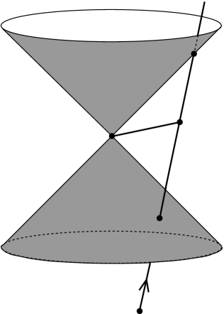
Figure 1: A timelike line $\ell=\{r+\lambda v\mid\lambda\in\mathbb{R}\}$ intersects the light-cone with vertex $p\not\in\ell$ in two points: $q_{+}$, its intersection with the future light-cone and $q_{-}$, its intersection with past the light cone. $q$ is a point in between $q_{+}$ and $q_{-}$.

Proposition 11.

Let $\ell$ and $\mathcal{L}_{p}$ as in Lemma 10 with $v$ timelike. Let $q_{+}$ and $q_{-}$ be the two intersection points of $\ell$ with $\mathcal{L}_{p}$ and $q\in\ell$ a point between them. Then

$$\|q-p\|_{g}^{2}=\|q_{+}-q\|_{g}\,\|q-q_{-}\|_{g}\,.$$ (52)

Moreover, $\|q_{+}-q\|_{g}=\|q-q_{-}\|_{g}$ iff $p-q$ is perpendicular to $v$.

Proof.

The vectors $(q_{+}-p)=(q-p)+(q_{+}-q)$ and $(q_{-}-p)=(q-p)+(q_{-}-q)$ are lightlike, which gives (note that $q-p$ is spacelike):

$$\|q-p\|_{g}^{2} \,=\,-(q-p)^{2} \,=\,(q_{+}-q)^{2}+2(q-p)\cdot(q_{+}-q)\,,$$ (53a)

$$\|q-p\|_{g}^{2} \,=\,-(q-p)^{2} \,=\,(q_{-}-q)^{2}+2(q-p)\cdot(q_{-}-q)\,.$$ (53b)

Since $q_{+}-q$ and $q-q_{-}$ are parallel we have $q_{+}-q=\lambda(q-q_{-})$ with $\lambda\in\mathbb{R}_{+}$ so that $(q_{+}-q)^{2}=\lambda\|q_{+}-q\|_{g}\|q-q_{-}\|_{g}$ and $\lambda(q_{-}-q)^{2}=\|q_{+}-q\|_{g}\|q-q_{-}\|_{g}$. Now, multiplying (53b) with $\lambda$ and adding this to (53a) immediately yields

$$(1+\lambda)\,\|q-p\|_{g}^{2}=(1+\lambda)\,\,\|q_{+}-q\|_{g}\|q-q_{-}\|_{g}\,.\\$$ (54)

Since $1+\lambda\neq 0$ this implies (52). Finally, since $q_{+}-q$ and $q_{-}-q$ are antiparallel, $\|q_{+}-q\|_{g}=\|q_{-}-q\|_{g}$ iff $(q_{+}-q)=-(q_{-}-q)$. Equations (53) now show that this is the case iff $(q-p)\cdot(q_{\pm}-q)=0$, i.e. iff $(q-p)\cdot v=0$. Hence we have shown

$$\|q_{+}-q\|_{g}=\|q-q_{-}\|_{g}\ \Longleftrightarrow\ (q-p)\cdot v=0\,.$$ (55)

In other words, $q$ is the midpoint of the segment $\overline{q_{+}q_{-}}$ iff the line through $p$ and $q$ is perpendicular (wrt. $g$) to $\ell$. ∎

The somewhat surprising feature of the first statement of this proposition is that (52) holds for any point of the segment $\overline{q_{+}q_{-}}$, not just the midpoint, as it would have to be the case for the corresponding statement in Euclidean geometry.

The second statement of Proposition 11 gives a convenient geometric characterisation of Einstein-simultaneity. Recall that an event $q$ on a timelike line $\ell$ (representing an inertial observer) is defined to be Einstein-simultaneous with an event $p$ in spacetime iff $q$ bisects the segment $\overline{q_{+}q_{-}}$ between the intersection points $q_{+},q_{-}$ of $\ell$ with the double-lightcone at $p$. Hence Proposition 11 implies

Corollary 12.

Einstein simultaneity with respect to a timelike line $\ell$ is an equivalence relation on spacetime, the equivalence classes of which are the spacelike hyperplanes orthogonal (wrt. $g$) to $\ell$.

The first statement simply follows from the fact that the family of parallel hyperplanes orthogonal to $\ell$ form a partition (cf. Sect. A.1) of spacetime.

From now on we shall use the terms ‘timelike line’ and ‘inertial observer’ synonymously. Note that Einstein simultaneity is only defined relative to an inertial observer. Given two inertial observers,

$$\ell \,=\,\{r+\lambda v\mid\lambda\in\mathbb{R}\}\qquad \text{first observer}\,,$$ (56a)

$$\ell^{\prime} \,=\,\{r^{\prime}+\lambda^{\prime}v^{\prime}\mid\lambda^{\prime}\in\mathbb{R}\}\qquad \text{second observer}\,,$$ (56b)

we call the corresponding Einstein-simultaneity relations $\ell$-simultaneity and $\ell^{\prime}$-simultaneity. Obviously they coincide iff $\ell$ and $\ell^{\prime}$ are parallel ($v$ and $v^{\prime}$ are linearly dependent). In this case $q^{\prime}\in\ell^{\prime}$ is $\ell$-simultaneous to $q\in\ell$ iff $q\in\ell$ is $\ell^{\prime}$-simultaneous to $q^{\prime}\in\ell^{\prime}$. If $\ell$ and $\ell^{\prime}$are not parallel (skew or intersecting in one point) it is generally not true that if $q^{\prime}\in\ell^{\prime}$ is $\ell$-simultaneous to $q\in\ell$ then $q\in\ell$ is also $\ell^{\prime}$-simultaneous to $q^{\prime}\in\ell^{\prime}$. In fact, we have

Proposition 13.

Let $\ell$ and $\ell^{\prime}$ two non-parallel timelike likes. There exists a unique pair $(q,q^{\prime})\in\ell\times\ell^{\prime}$ so that $q^{\prime}$ is $\ell$-simultaneous to $q$ and $q$ is $\ell^{\prime}$ simultaneous to $q^{\prime}$.

Proof.

We parameterise $\ell$ and $\ell^{\prime}$ as in (56). The two conditions for $q^{\prime}$ being $\ell$-simultaneous to $q$ and $q$ being $\ell^{\prime}$-simultaneous to $q^{\prime}$ are $(q-q^{\prime})\cdot v=0=(q-q^{\prime})\cdot v^{\prime}$. Writing $q=r+\lambda v$ and $q^{\prime}=r^{\prime}+\lambda^{\prime}v^{\prime}$ this takes the form of the following matrix equation for the two unknowns $\lambda$ and $\lambda^{\prime}$:

$$\begin{pmatrix}v^{2}&-v\cdot v^{\prime}\\ v\cdot v^{\prime}&-v^{\prime 2}\end{pmatrix}\begin{pmatrix}\lambda\\ \lambda^{\prime}\end{pmatrix}=\begin{pmatrix}(r^{\prime}-r)\cdot v\\ (r^{\prime}-r)\cdot v^{\prime}\end{pmatrix}\,.$$ (57)

This has a unique solution pair $(\lambda,\lambda^{\prime})$, since for linearly independent timelike vectors $v$ and $v^{\prime}$ Lemma 9 implies $(v\cdot v^{\prime})^{2}-v^{2}v^{\prime 2}>0$. Note that if $\ell$ and $\ell^{\prime}$ intersect $q=q^{\prime}=\text{intersection point}$. ∎

Clearly, Einstein-simultaneity is conventional and physics proper should not depend on it. For example, the fringe-shift in the Michelson-Morley experiment is independent of how we choose to synchronise clocks. In fact, it does not even make use of any clock. So what is the general definition of a ‘simultaneity structure’? It seems obvious that it should be a relation on spacetime that is at least symmetric (each event should be simultaneous to itself). Going from one-way simultaneity to the mutual synchronisation of two clocks, one might like to also require reflexivity (if $p$ is simultaneous to $q$ then $q$ is simultaneous to $p$), though this is not strictly required in order to one-way synchronise each clock in a set of clocks with one preferred ‘master clock’, which is sufficient for many applications.

Moreover, if we like to speak of the mutual simultaneity of sets of more than two events we need an equivalence relation on spacetime. The equivalence relation should be such that each inertial observer intersect each equivalence class precisely once. Let us call such a simultaneity structure ‘admissible’. Clearly there are zillions of such structures: just partition spacetime into any set of appropriate spacelike hypersurfaces (there are more possibilities at this point, like families of forward or backward lightcones). An absolute admissible simultaneity structure would be one which is invariant (cf. Sect. A.1) under the automorphism group of spacetime. We have

Proposition 14.

There exits precisely one admissible simultaneity structure which is invariant under the inhomogeneous proper orthochronous Galilei group and none that is invariant under the inhomogeneous proper orthochronous Lorentz group.

A proof is given in [24]. There is a group-theoretic reason that highlights this existential difference:

Proposition 15.

Let $G$ be a group with transitive action on a set $S$. Let $\mathrm{Stab}(p)\subset G$ be the stabiliser subgroup for $p\in S$ (due to transitivity all stabiliser subgroups are conjugate). Then $S$ admits a $G$-invariant equivalence relation $R\subset S\times S$ iff $\mathrm{Stab}(p)$ is not maximal, that is, iff $\mathrm{Stab}(p)$ is properly contained in a proper subgroup $H$ of $G$: $\mathrm{Stab}(p)\subsetneq H\subsetneq G$.

A proof of this may be found in [31] (Theorem 1.12). Regarding the action of the inhomogeneous Galilei and Lorentz groups on spacetime, their stabilisers are the corresponding homogeneous groups. Now, the homogeneous Lorentz group is maximal in the inhomogeneous one, whereas the homogeneous Galilei group is not maximal in the inhomogeneous one, since it can still be supplemented by time translations without the need to also invoke space translations. This, according to Proposition 15, is the group theoretic origin of the absence of any invariant simultaneity structure in the Lorentzian case.

However, one may ask whether there are simultaneity structures relative to some additional structure $X$. As additional structure, $X$, one could, for example, take an inertial reference frame, which is characterised by a foliation of spacetime by parallel timelike lines. The stabiliser subgroup of that structure within the proper orthochronous Poincaré group is given by the semidirect product of spacetime translations with all rotations in the hypersurfaces perpendicular to the lines in $X$:

$$\mathrm{Stab}_{X}(\mathsf{ILor}_{\uparrow+})\cong\mathbb{R}^{4}\rtimes\mathsf{SO}(3)\,.$$ (58)

Here the $\mathsf{SO}(3)$ only acts on the spatial translations, so that the group is also isomorphic to $\mathbb{R}\times\mathsf{E}(3)$, where $\mathsf{E}(3)$ is the group of Euclidean motions in 3-dimensions (the hyperplanes perpendicular to the lines in $X$). We can now ask: how many admissible $\mathrm{Stab}_{X}(\mathsf{ILor}_{\uparrow+})$ – invariant equivalence relations are there. The answer is

Proposition 16.

There exits precisely one admissible simultaneity structure which is invariant under $\mathrm{Stab}_{X}(\mathsf{ILor}_{\uparrow+})$, where $X$ represents am inertial reference frame (a foliation of spacetime by parallel timelike lines). It is given by Einstein simultaneity, that is, the equivalence classes are the hyperplanes perpendicular to the lines in $X$.

The proof is given in [24]. Note again the connection to quoted group-theoretic result: The stabiliser subgroup of a point in $\mathrm{Stab}_{X}(\mathsf{ILor}_{\uparrow+})$ is $\mathsf{SO(3)}$, which is clearly not maximal in $\mathrm{Stab}_{X}(\mathsf{ILor}_{\uparrow+})$ since it is a proper subgroup of $\mathsf{E}(3)$ which, in turn, is a proper subgroup of $\mathrm{Stab}_{X}(\mathsf{ILor}_{\uparrow+})$.

3.2 The lattices of causally and chronologically complete sets

Here we wish to briefly discuss another important structure associated with causality relations in Minkowski space, which plays a fundamental rôle in modern Quantum Field Theory (see e.g. [27]). Let $S_{1}$ and $S_{2}$ be subsets of $\mathbb{M}^{n}$. We say that $S_{1}$ and $S_{2}$ are causally disjoint or spacelike separated iff $p_{1}-p_{2}$ is spacelike, i.e. $(p_{1}-p_{2})^{2}<0$, for any $p_{1}\in S_{1}$ and $p_{2}\in S_{2}$. Note that because a point is not spacelike separated from itself, causally disjoint sets are necessarily disjoint in the ordinary set-theoretic sense—the converse being of course not true.

For any subset $S\subseteq\mathbb{M}^{n}$ we denote by $S^{\prime}$ the largest subset of $\mathbb{M}^{n}$ which is causally disjoint to $S$. The set $S^{\prime}$ is called the causal complement of $S$. The procedure of taking the causal complement can be iterated and we set $S^{\prime\prime}:=(S^{\prime})^{\prime}$ etc. $S^{\prime\prime}$ is called the causal completion of $S$. It also follows straight from the definition that $S_{1}\subseteq S_{2}$ implies $S^{\prime}_{1}\supseteq S^{\prime}_{2}$ and also $S^{\prime\prime}\supseteq S$. If $S^{\prime\prime}=S$ we call $S$ causally complete. We note that the causal complement $S^{\prime}$ of any given $S$ is automatically causally complete. Indeed, from $S^{\prime\prime}\supseteq S$ we obtain $(S^{\prime})^{\prime\prime}\subseteq S^{\prime}$, but the first inclusion applied to $S^{\prime}$ instead of $S$ leads to $(S^{\prime})^{\prime\prime}\supseteq S^{\prime}$, showing $(S^{\prime})^{\prime\prime}=S^{\prime}$. Note also that for any subset $S$ its causal completion, $S^{\prime\prime}$, is the smallest causally complete subset containing $S$, for if $S\subseteq K\subseteq S^{\prime\prime}$ with $K^{\prime\prime}=K$, we derive from the first inclusion by taking ^′′ that $S^{\prime\prime}\subseteq K$, so that the second inclusion yields $K=S^{\prime\prime}$. Trivial examples of causally complete subsets of $\mathbb{M}^{n}$ are the empty set, single points, and the total set $\mathbb{M}^{n}$. Others are the open diamond-shaped regions (15) as well as their closed counterparts:

$$\bar{U}(p,q):=(\mathcal{\bar{C}}^{+}_{p}\cap\mathcal{\bar{C}}^{-}_{q})\cup(\mathcal{\bar{C}}^{+}_{q}\cap\mathcal{\bar{C}}^{-}_{p})\,.$$ (59)

We now focus attention to the set $\mathrm{Caus}(\mathbb{M}^{n})$ of causally complete subsets of $\mathbb{M}^{n}$, including the empty set, $\emptyset$, and the total set, $\mathbb{M}^{n}$, which are mutually causally complementary. It is partially ordered by ordinary set-theoretic inclusion $(\subseteq)$ (cf. Sect. A.1) and carries the ‘dashing operation’ $(^{\prime})$ of taking the causal complement. Moreover, on $\mathrm{Caus}(\mathbb{M}^{n})$ we can define the operations of ‘meet’ and ‘join’, denoted by $\wedge$ and $\vee$ respectively, as follows: Let $S_{i}\in\mathrm{Caus}(\mathbb{M}^{n})$ where $i=1,2$, then $S_{1}\wedge S_{2}$ is the largest causally complete subset in the intersection $S_{1}\cap S_{2}$ and $S_{1}\vee S_{2}$ is the smallest causally complete set containing the union $S_{1}\cup S_{2}$.

The operations of $\wedge$ and $\vee$ can be characterised in terms of the ordinary set-theoretic intersection $\cap$ together with the dashing-operation. To see this, consider two causally complete sets, $S_{i}$ where $i=1,2$, and note that the set of points that are spacelike separated from $S_{1}$ and $S_{2}$ are obviously given by $S^{\prime}_{1}\cap S^{\prime}_{2}$, but also by $(S_{1}\cup S_{2})^{\prime}$, so that

$$S^{\prime}_{1}\cap S^{\prime}_{2} \,=\,(S_{1}\cup S_{2})^{\prime}\,,$$ (60a)

$$S_{1}\cap S_{2} \,=\,(S^{\prime}_{1}\cup S^{\prime}_{2})^{\prime}\,.$$ (60b)

Here (60a) and (60b) are equivalent since any $S_{i}\in\mathrm{Caus}(\mathbb{M}^{n})$ can be written as $S_{i}=P^{\prime}_{i}$, namely $P_{i}=S^{\prime}_{i}$. If $S_{i}$ runs through all sets in $\mathrm{Caus}(\mathbb{M}^{n})$ so does $P_{i}$. Hence any equation that holds generally for all $S_{i}\in\mathrm{Caus}(\mathbb{M}^{n})$ remains valid if the $S_{i}$ are replaced by $S^{\prime}_{i}$.

Equation (60b) immediately shows that $S_{1}\cap S_{2}$ is causally complete (since it is the ^′ of something). Taking the causal complement of (60a) we obtain the desired relation for $S_{1}\vee S_{2}:=(S_{1}\cup S_{2})^{\prime\prime}$. Together we have

$$S_{1}\wedge S_{2} \,=\,S_{1}\cap S_{2}\,,$$ (61a)

$$S_{1}\vee S_{2} \,=\,(S^{\prime}_{1}\cap S^{\prime}_{2})^{\prime}\,.$$ (61b)

From these we immediately derive

$$(S_{1}\wedge S_{2})^{\prime} \,=\,S^{\prime}_{1}\vee S^{\prime}_{2}\,,$$ (62a)

$$(S_{1}\vee S_{2})^{\prime} \,=\,S^{\prime}_{1}\wedge S^{\prime}_{2}\,.$$ (62b)

All what we have said so far for the set $\mathrm{Caus}(\mathbb{M}^{n})$ could be repeated verbatim for the set $\mathrm{Chron}(\mathbb{M}^{n})$ of chronologically complete subsets. We say that $S_{1}$ and $S_{2}$ are chronologically disjoint or non-timelike separated, iff $S_{1}\cap S_{2}=\emptyset$ and $(p_{1}-p_{2})^{2}\leq 0$ for any $p_{1}\in S_{1}$ and $p_{2}\in S_{2}$. $S^{\prime}$, the chronological complement of $S$, is now the largest subset of $\mathbb{M}^{n}$ which is chronologically disjoint to $S$. The only difference between the causal and the chronological complement of $S$ is that the latter now contains lightlike separated points outside $S$. A set $S$ is chronologically complete iff $S=S^{\prime\prime}$, where the dashing now denotes the operation of taking the chronological complement. Again, for any set $S$ the set $S^{\prime}$ is automatically chronologically complete and $S^{\prime\prime}$ is the smallest chronologically complete subset containing $S$. Single points are chronologically complete subsets. All the formal properties regarding ^′, $\wedge$, and $\vee$ stated hitherto for $\mathrm{Caus}(\mathbb{M}^{n})$ are the same for $\mathrm{Chron}(\mathbb{M}^{n})$.

One major difference between $\mathrm{Caus}(\mathbb{M}^{n})$ and $\mathrm{Chron}(\mathbb{M}^{n})$ is that the types of diamond-shaped sets they contain are different. For example, the closed ones, (59), are members of both. The open ones, (15), are contained in $\mathrm{Caus}(\mathbb{M}^{n})$ but not in $\mathrm{Chron}(\mathbb{M}^{n})$. Instead, $\mathrm{Chron}(\mathbb{M}^{n})$ contains the closed diamonds whose ‘equator’ have been removed. An essential structural difference between $\mathrm{Caus}(\mathbb{M}^{n})$ and $\mathrm{Chron}(\mathbb{M}^{n})$ will be stated below, after we have introduced the notion of a lattice to which we now turn.

To put all these formal properties into the right frame we recall the definition of a lattice. Let $(L,\leq)$ be a partially ordered set and $a,b$ any two elements in $L$. Synonymously with $a\leq b$ we also write $b\geq a$ and say that $a$ is smaller than $b$, $b$ is bigger than $a$, or $b$ majorises $a$. We also write $a<b$ if $a\leq b$ and $a\neq b$. If, with respect to $\leq$, their greatest lower and least upper bound exist, they are denoted by $a\wedge b$—called the ‘meet of $a$ and $b$’—and $a\vee b$—called the ‘join of $a$ and $b$’—respectively. A partially ordered set for which the greatest lower and least upper bound exist for any pair $a,b$ of elements from $L$ is called a lattice.

We now list some of the most relevant additional structural elements lattices can have: A lattice is called complete if greatest lower and least upper bound exist for any subset $K\subseteq L$. If $K=L$ they are called $0$ (the smallest element in the lattice) and $1$ (the biggest element in the lattice) respectively. An atom in a lattice is an element $a$ which majorises only $0$, i.e. $0\leq a$ and if $0\leq b\leq a$ then $b=0$ or $b=a$. The lattice is called atomic if each of its elements different from $0$ majorises an atom. An atomic lattice is called atomistic if every element is the join of the atoms it majorises. An element $c$ is said to cover $a$ if $a<c$ and if $a\leq b\leq c$ either $a=b$ or $b=c$. An atomic lattice is said to have the covering property if, for every element $b$ and every atom $a$ for which $a\wedge b=0$, the join $a\vee b$ covers $b$.

The subset $\{a,b,c\}\subseteq L$ is called a distributive triple if

$$a\wedge(b\vee c) \,=\,(a\wedge b)\vee(a\wedge c)\quad \text{and $(a,b,c)$ cyclically permuted}\,,$$ (63a)

$$a\vee(b\wedge c) \,=\,(a\vee b)\wedge(a\vee c)\quad \text{and $(a,b,c)$ cyclically permuted}\,.$$ (63b)

Definition 4.

A lattice is called distributive or Boolean if every triple $\{a,b,c\}$ is distributive. It is called modular if every triple $\{a,b,c\}$ with $a\leq b$ is distributive.

It is straightforward to check from (63) that modularity is equivalent to the following single condition:

$$\text{modularity}\Leftrightarrow a\vee(b\wedge c)=b\wedge(a\vee c)\quad\text{for all $a,b,c\in L$ s.t. $a\leq b$.}$$ (64)

If in a lattice with smallest element $0$ and greatest element $1$ a map $L\rightarrow L$, $a\mapsto a^{\prime}$, exist such that

$$a^{\prime\prime}:=(a^{\prime})^{\prime}=a\,,$$ (65a)

$$a\leq b\Rightarrow b^{\prime}\leq a^{\prime}\,,$$ (65b)

$$a\wedge a^{\prime}=0\,,\quad a\vee a^{\prime}=1\,,$$ (65c)

the lattice is called orthocomplemented. It follows that whenever the meet and join of a subset $\{a_{i}\mid i\in I\}$ ($I$ is some index set) exist one has De Morgan’s laws:

$$\bigl{(}\textstyle{\bigwedge_{i\in I}}\ a_{i}\bigr{)}^{\prime} \,=\,\textstyle{\bigvee_{i\in I}}\ a^{\prime}_{i}\,,$$ (66a)

$$\bigl{(}\textstyle{\bigvee_{i\in I}}\ a_{i}\bigr{)}^{\prime} \,=\,\textstyle{\bigwedge_{i\in I}}\ a^{\prime}_{i}\,.$$ (66b)

For orthocomplemented lattices there is a still weaker version of distributivity than modularity, which turns out to be physically relevant in various contexts:

Definition 5.

An orthocomplemented lattice is called orthomodular if every triple $\{a,b,c\}$ with $a\leq b$ and $c\leq b^{\prime}$ is distributive.

From (64) and using that $b\wedge c=0$ for $b\leq c^{\prime}$ one sees that this is equivalent to the single condition (renaming $c$ to $c^{\prime}$):

orthomod. $$\Leftrightarrow\quad a\,=\,b\wedge(a\vee c^{\prime})\quad a,b,c\in L a\leq b\leq c$$ for all s.t.  , (67a)

$$\Leftrightarrow a\,=\,b\vee(a\wedge c^{\prime})\quad a,b,c\in L a\geq b\geq c$$ for all s.t.  , (67b)

where the second line follows from the first by taking its orthocomplement and renaming $a^{\prime},b^{\prime},c$ to $a,b,c^{\prime}$. It turns out that these conditions can still be simplified by making them independent of $c$. In fact, (67) are equivalent to

orthomod. $$\Leftrightarrow\quad a=b\wedge(a\vee b^{\prime})\quad a,b\in L a\leq b$$ for all s.t.  , (68a)

$$\Leftrightarrow a=b\vee(a\wedge b^{\prime})\quad a,b\in L a\geq b$$ for all s.t.  . (68b)

It is obvious that (67) implies (68) (set $c=b$). But the converse is also true. To see this, take e.g. (68b) and choose any $c\leq b$. Then $c^{\prime}\geq b^{\prime}$, $a\geq b$ (by hypothesis), and $a\geq a\wedge c^{\prime}$ (trivially), so that $a\geq b\vee(a\wedge c^{\prime})$. Hence $a\geq b\vee(a\wedge c^{\prime})\geq b\vee(a\wedge b^{\prime})=a$, which proves (67b).

Complete orthomodular atomic lattices are automatically atomistic. Indeed, let $b$ be the join of all atoms majorised by $a\neq 0$. Assume $a\neq b$ so that necessarily $b<a$, then (68b) implies $a\wedge b^{\prime}\neq 0$. Then there exists an atom $c$ majorised by $a\wedge b^{\prime}$. This implies $c\leq a$ and $c\leq b^{\prime}$, hence also $c\not\leq b$. But this is a contradiction, since $b$ is by definition the join of all atoms majorised by $a$.

Finally we mention the notion of compatibility or commutativity, which is a symmetric, reflexive, but generally not transitive relation $R$ on an orthomodular lattice (cf. Sec. A.1). We write $a\natural b$ for $(a,b)\in R$ and define:

$$a\natural b\quad \Leftrightarrow\quad a \,=\,(a\wedge b)\vee(a\wedge b^{\prime})\,,$$ (69a)

$$\Leftrightarrow\quad b \,=\,(b\wedge a)\vee(b\wedge a^{\prime})\,.$$ (69b)

The equivalence of these two lines, which shows that the relation of being compatible is indeed symmetric, can be demonstrated using orthomodularity as follows: Suppose (69a) holds; then $b\wedge a^{\prime}=b\wedge(b^{\prime}\vee a^{\prime})\wedge(b\vee a^{\prime})=b\wedge(b^{\prime}\vee a^{\prime})$, where we used the orthocomplement of (69a) to replace $a^{\prime}$ in the first expression and the trivial identity $b\wedge(b\vee a^{\prime})=b$ in the second step. Now, applying (68b) to $b\geq a\wedge b$ we get $b=(b\wedge a)\vee[b\wedge(b^{\prime}\vee a^{\prime})]=(b\wedge a)\vee(b\wedge a^{\prime})$, i.e. (69b). The converse, $(\ref{eq:DefCompatibility2})\Rightarrow(\ref{eq:DefCompatibility1})$, is of course entirely analogous.

From (69) a few things are immediate: $a\natural b$ is equivalent to $a\natural b^{\prime}$, $a\natural b$ is implied by $a\leq b$ or $a\leq b^{\prime}$, and the elements $0$ and $1$ are compatible with all elements in the lattice. The centre of a lattice is the set of elements which are compatible with all elements in the lattice. In fact, the centre is a Boolean sublattice. If the centre contains no other elements than $0$ and $1$ the lattice is said to be irreducible. The other extreme is a Boolean lattice, which is identical to its own centre. Indeed, if $(a,b,b^{\prime})$ is a distributive triple, one has $a=a\wedge 1=a\wedge(b\vee b^{\prime})=(a\wedge b)\vee(a\wedge b^{\prime})\Rightarrow(\ref{eq:DefCompatibility1})$.

After these digression into elementary notions of lattice theory we come back to our examples of the sets $\mathrm{Caus}(\mathbb{M}^{n})$ $\mathrm{Chron}(\mathbb{M}^{n})$. Our statements above amount to saying that they are complete, atomic, and orthocomplemented lattices. The partial order relation $\leq$ is given by $\subseteq$ and the extreme elements $0$ and $1$ correspond to the empty set $\emptyset$ and the total set $\mathbb{M}^{n}$, the points of which are the atoms. Neither the covering property nor modularity is shared by any of the two lattices, as can be checked by way of elementary counterexamples. In particular, neither of them is Boolean. However, in [15] it was shown that $\mathrm{Chron}(\mathbb{M}^{n})$ is orthomodular; see also [13] which deals with more general spacetimes. Note that by the argument given above this implies that $\mathrm{Chron}(\mathbb{M}^{n})$ is atomistic. In contrast, $\mathrm{Caus}(\mathbb{M}^{n})$ is definitely not orthomodular, as is e.g. seen by the counterexample given in Fig. 2. It is also not difficult to prove that $\mathrm{Chron}(\mathbb{M}^{n})$ is irreducible.

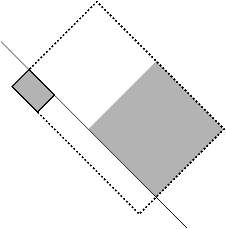
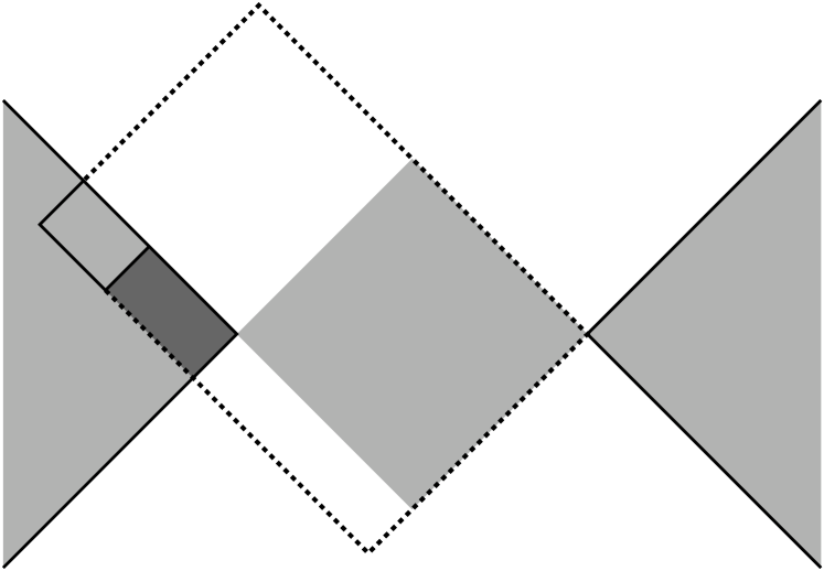
Figure 2: The two figures show that $\text{Caus}(\mathbb{M}^{n})$ is not orthomodular. The first thing to note is that $\text{Caus}(\mathbb{M}^{n})$ contains open (15) as well as closed (59) diamond sets. In the left picture we consider the join of a small closed diamond $a$ with a large open diamond $b^{\prime}$. (Closed sets are indicated by a solid boundary line.) Their edges are aligned along the lightlike line $\ell$. Even though these regions are causally disjoint, their causal completion is much larger than their union and given by the open (for $n>2$) enveloping diamond $a\vee b^{\prime}$ framed by the dashed line. (This also shows that the join of two regions can be larger than the domain of dependence of their union; compare footnote 19.) . Next we consider the situation depicted on the right side. The closed double-wedge region $b$ contains the small closed diamond $a$. The causal complement $b^{\prime}$ of $b$ is the open diamond in the middle. $a\vee b^{\prime}$ is, according to the first picture, given by the large open diamond enclosed by the dashed line. The intersection of $a\vee b^{\prime}$ with $b$ is strictly larger than $a$, the difference being the dark-shaded region in the left wedge of $b$ below $a$. Hence $a\neq b\wedge(a\vee b^{\prime})$, in contradiction to (68a).

It is well known that the lattices of propositions for classical systems are Boolean, whereas those for quantum systems are merely orthomodular. In classical physics the elements of the lattice are measurable subsets of phase space, with $\leq$ being ordinary set-theoretic inclusion $\subseteq$, and $\wedge$ and $\vee$ being ordinary set-theoretic intersection $\cap$ and union $\cup$ respectively. The orthocomplement is the ordinary set-theoretic complement. In Quantum Mechanics the elements of the lattice are the closed subspaces of Hilbert space, with $\leq$ being again ordinary inclusion, $\wedge$ ordinary intersection, and $\vee$ is given by $a\vee b:=\overline{\mbox{span}\{a,b\}}$. The orthocomplement of a closed subset is the orthogonal complement in Hilbert space. For comprehensive discussions see [33] and [4].

One of the main questions in the foundations of Quantum Mechanics is whether one could understand (derive) the usage of Hilbert spaces and complex numbers from somehow more fundamental principles. Even though it is not a priori clear what ones measure of fundamentality should be at this point, an interesting line of attack consists in deriving the mentioned structures from the properties of the lattice of propositions (Quantum Logic). It can be shown that a lattice that is complete, atomic, irreducible, orthomodular, and that satisfies the covering property is isomorphic to the lattice of closed subspaces of a linear space with Hermitean inner product. The complex numbers are selected if additional technical assumptions are added. For the precise statements of these reconstruction theorems see [4].

It is now interesting to note that, on a formal level, there is a similar transition in going from Galilei invariant to Lorentz invariant causality relations. In fact, in Galilean spacetime one can also define a chronological complement: Two points are chronologically related if they are connected by a worldline of finite speed and, accordingly, two subsets in spacetime are chronologically disjoint if no point in one set is chronologically related to a point of the other. For example, the chronological complement of a point $p$ are all points simultaneous to, but different from, $p$. More general, it is not hard to see that the chronologically complete sets are just the subsets of some $t=\text{const.}$ hypersurface. The lattice of chronologically complete sets is then the continuous disjoint union of sublattices, each of which is isomorphic to the Boolean lattice of subsets in $\mathbb{R}^{3}$. For details see [14].

As we have seen above, $\text{Chron}(\mathbb{M}^{n})$ is complete, atomic, irreducible, and orthomodular (hence atomistic). The main difference to the lattice of propositions in Quantum Mechanics, as regards the formal aspects discussed here, is that $\text{Chron}(\mathbb{M}^{n})$ does not satisfy the covering property. Otherwise the formal similarities are intriguing and it is tempting to ask whether there is a deeper meaning to this. In this respect it would be interesting to know whether one could give a lattice-theoretic characterisation for $\text{Chron}(M)$ ($M$ some fixed spacetime), comparable to the characterisation of the lattices of closed subspaces in Hilbert space alluded to above. Even for $M=\mathbb{M}^{n}$ such a characterisation seems, as far as I am aware, not to be known.

3.3 Rigid motion

As is well known, the notion of a rigid body, which proves so useful in Newtonian mechanics, is incompatible with the existence of a universal finite upper bound for all signal velocities [36]. As a result, the notion of a perfectly rigid body does not exist within the framework of SR. However, the notion of a rigid motion does exist. Intuitively speaking, a body moves rigidly if, locally, the relative spatial distances of its material constituents are unchanging.

The motion of an extended body is described by a normalised timelike vector field $u:\Omega\rightarrow\mathbb{R}^{n}$, where $\Omega$ is an open subset of Minkowski space, consisting of the events where the material body in question ‘exists’. We write $g(u,u)=u\cdot u=u^{2}$ for the Minkowskian scalar product. Being normalised now means that $u^{2}=c^{2}$ (we do not choose units such that $c=1$). The Lie derivative with respect to $u$ is denoted by $L_{u}$.

For each material part of the body in motion its local rest space at the event $p\in\Omega$ can be identified with the hyperplane through $p$ orthogonal to $u_{p}$:

$$H_{p}:=p+u_{p}^{\perp}\,.$$ (70)

$u_{p}^{\perp}$ carries a Euclidean inner product, $h_{p}$, given by the restriction of $-g$ to $u_{p}^{\perp}$. Generally we can write

$$h=c^{-2}\,u^{\flat}\otimes u^{\flat}-g\,,$$ (71)

where $u^{\flat}=g^{\downarrow}(u):=g(u,\cdot)$ is the one-form associated to $u$. Following [9] the precise definition of ‘rigid motion’ can now be given as follows:

Definition 6 (Born 1909).

Let $u$ be a normalised timelike vector field $u$. The motion described by its flow is rigid if

$$L_{u}h=0\,.$$ (72)

Note that, in contrast to the Killing equations $L_{u}g=0$, these equations are non linear due to the dependence of $h$ upon $u$.

We write $\Pi_{h}:=\text{id}-c^{-2}\,u\otimes u^{\flat}\in\mbox{End}(\mathbb{R}^{n})$ for the tensor field over spacetime that pointwise projects vectors perpendicular to $u$. It acts on one forms $\alpha$ via $\Pi_{h}(\alpha):=\alpha\circ\Pi_{h}$ and accordingly on all tensors. The so extended projection map will still be denoted by $\Pi_{h}$. Then we e.g. have

$$h=-\Pi_{h}g:=-g(\Pi_{h}\cdot,\Pi_{h}\cdot)\,.$$ (73)

It is not difficult to derive the following two equations:

$$L_{fu}h \,=\,fL_{u}h\,,$$ (74)

$$L_{u}h \,=\,-L_{u}(\Pi_{h}g)=-\Pi_{h}(L_{u}g)\,,$$ (75)

where $f$ is any differentiable real-valued function on $\Omega$.

Equation (74) shows that the normalised vector field $u$ satisfies (72) iff any rescaling $fu$ with a nowhere vanishing function $f$ does. Hence the normalization condition for $u$ in (72) is really irrelevant. It is the geometry in spacetime of the flow lines and not their parameterisation which decide on whether motions (all, i.e. for any parameterisation, or none) along them are rigid. This has be the case because, generally speaking, there is no distinguished family of sections (hypersurfaces) across the bundle of flow lines that would represent ‘the body in space’, i.e. mutually simultaneous locations of the body’s points. Distinguished cases are those exceptional ones in which $u$ is hypersurface orthogonal. Then the intersection of $u$’s flow lines with the orthogonal hypersurfaces consist of mutually Einstein synchronous locations of the points of the body. An example is discussed below.

Equation (75) shows that the rigidity condition is equivalent to the ‘spatially’ projected Killing equation. We call the flow of the timelike normalised vector field $u$ a Killing motion (i.e. a spacetime isometry) if there is a Killing field $K$ such that $u=cK/\sqrt{K^{2}}$. Equation (75) immediately implies that Killing motions are rigid. What about the converse? Are there rigid motions that are not Killing? This turns out to be a difficult question. Its answer in Minkowski space is: ‘yes, many, but not as many as naïvely expected.’

Before we explain this, let us give an illustrative example for a Killing motion, namely that generated by the boost Killing-field in Minkowski space. We suppress all but one spatial directions and consider boosts in $x$ direction in two-dimensional Minkowski space (coordinates $ct$ and $x$; metric $ds^{2}=c^{2}dt^{2}-dx^{2}$). The Killing field is

$$K=x\,\partial_{ct}+ct\,\partial_{x}\,,$$ (76)

which is timelike in the region $|x|>|ct|$. We focus on the ‘right wedge’ $x>|ct|$, which is now our region $\Omega$. Consider a rod of length $\ell$ which at $t=0$ is represented by the interval $x\in(r,r+\ell)$, where $r>0$. The flow of the normalised field $u=cK/\sqrt{K^{2}}$ is

$$ct(\tau) \,=\,x_{0}\,\sinh\bigl{(}c\tau/x_{0})\,,$$ (77a)

$$x(\tau) \,=\,x_{0}\,\cosh\bigl{(}c\tau/x_{0})\,,$$ (77b)

where $x_{0}=x(\tau=0)\in(r,r+\ell)$ labels the elements of the rod at $\tau=0$. We have $x^{2}-c^{2}t^{2}=x_{0}^{2}$, showing that the individual elements of the rod move on hyperbolae (‘hyperbolic motion’). $\tau$ is the proper time along each orbit, normalised so that the rod lies on the $x$ axis at $\tau=0$.

The combination

$$\lambda:=c\tau/x_{0}$$ (78)

is just the flow parameter for $K$ (76), sometimes referred to as ‘Killing time’ (though it is dimensionless). From (77) we can solve for $\lambda$ and $\tau$ as functions of $ct$ and $x$:

$$\lambda \,=\,f(ct,x) \,:=\,\tanh^{-1}\bigl{(}ct/x\bigr{)}\,,$$ (79a)

$$\tau \,=\,\hat{f}(ct,x) \,:=\,\underbrace{\sqrt{(x/c)^{2}-t^{2}}}_{x_{0}/c}\,\tanh^{-1}\bigl{(}ct/x\bigr{)}\,,$$ (79b)

from which we infer that the hypersurfaces of constant $\lambda$ are hyperplanes which all intersect at the origin. Moreover, we also have $df=K^{\flat}/K^{2}$ ($d$ is just the ordinary exterior differential) so that the hyperplanes of constant $\lambda$ intersect all orbits of $u$ (and $K$) orthogonally. Hence the hyperplanes of constant $\lambda$ qualify as the equivalence classes of mutually Einstein-simultaneous events in the region $x>|ct|$ for a family of observers moving along the Killing orbits. This does not hold for the hypersurfaces of constant $\tau$, which are curved.

The modulus of the spacetime-acceleration (which is the same as the modulus of the spatial acceleration measured in the local rest frame) of the material part of the rod labelled by $x_{0}$ is

$$\|a\|_{g}=c^{2}/x_{0}\,.$$ (80)

As an aside we generally infer from this that, given a timelike curve of local acceleration (modulus) $\alpha$, infinitesimally nearby orthogonal hyperplanes intersect at a spatial distance $c^{2}/\alpha$. This remark will become relevant in the discussion of part 2 of the Noether-Herglotz theorem given below.

In order to accelerate the rod to the uniform velocity $v$ without deforming it, its material point labelled by $x_{0}$ has to accelerate for the eigentime (this follows from (77))

$$\tau=\frac{x_{0}}{c}\tanh^{-1}(v/c)\,,$$ (81)

which depends on $x_{0}$. In contrast, the Killing time is the same for all material points and just given by the final rapidity. In particular, judged from the local observers moving with the rod, a rigid acceleration requires accelerating the rod’s trailing end harder but shorter than pulling its leading end.

In terms of the coordinates $(\lambda,x_{0})$, which are co-moving with the flow of $K$, and $(\tau,x_{0})$, which are co-moving with the flow of $u$, we just have $K=\partial/\partial\lambda$ and $u=\partial/\partial\tau$ respectively. The spacetime metric $g$ and the projected metric $h$ in terms of these coordinates are:

$$h \,=\,dx_{0}^{2}\,,$$ (82a)

$$g \,=\,x_{0}^{2}\,d\lambda^{2}-dx_{0}^{2}=c^{2}\bigl{(}d\tau-(\tau/x_{0})\,dx_{0}\bigr{)}^{2}-dx_{0}^{2}\,.$$ (82b)

Note the simple form $g$ takes in terms of $x_{0}$ and $\lambda$, which are also called the ‘Rindler coordinates’ for the region $|x|>|ct|$ of Minkowski space. They are the analogs in Lorentzian geometry to polar coordinates (radius $x_{0}$, angle $\lambda$) in Euclidean geometry.

Let us now return to the general case. We decompose the derivative of the velocity one-form $u^{\flat}:=g^{\downarrow}(u)$ as follows:

$$\nabla u^{\flat}=\theta+\omega+c^{-2}\,u^{\flat}\otimes a^{\flat}\,,$$ (83)

where $\theta$ and $\omega$ are the projected symmetrised and antisymmetrised derivatives respectively

$$2\theta \,=\,\Pi_{h}(\nabla\vee u^{\flat}) \,=\,\nabla\vee u^{\flat}-c^{-2}\,u^{\flat}\vee a^{\flat}\,,$$ (84a)

$$2\omega \,=\,\Pi_{h}(\nabla\wedge u^{\flat}) \,=\,\nabla\wedge u^{\flat}-c^{-2}\,u^{\flat}\wedge a^{\flat}\,.$$ (84b)

The symmetric part, $\theta$, is usually further decomposed into its traceless and pure trace part, called the shear and expansion of $u$ respectively. The antisymmetric part $\omega$ is called the vorticity of $u$.

Now recall that the Lie derivative of $g$ is just twice the symmetrised derivative, which in our notation reads:

$$L_{u}g=\nabla\vee u^{\flat}\,.$$ (85)

This implies in view of (72), (75), and (84a)

Proposition 17.

Let $u$ be a normalised timelike vector field $u$. The motion described by its flow is rigid iff $u$ is of vanishing shear and expansion, i.e. iff $\theta=0$.

Vector fields generating rigid motions are now classified according to whether or not they have a vanishing vorticity $\omega$: if $\omega=0$ the flow is called irrotational, otherwise rotational. The following theorem is due to Herglotz [29] and Noether [40]:

Theorem 18 (Noether & Herglotz, part 1).

A rotational rigid motion in Minkowski space must be a Killing motion.

An example of such a rotational motion is given by the Killing field

$$K=\partial_{t}+\kappa\,\partial_{\varphi}$$ (86)

inside the region

$$\Omega=\{(t,z,\rho,\varphi)\mid\kappa\rho<c\}\,,$$ (87)

where $K$ is timelike. This motion corresponds to a rigid rotation with constant angular velocity $\kappa$ which, without loss of generality, we take to be positive. Using the co-moving angular coordinate $\psi:=\varphi-\kappa t$, the split (71) is now furnished by

$$u^{\flat} \,=\,c\,\sqrt{1-(\kappa\rho/c)^{2}}\left\{c\,dt-\frac{\kappa\rho/c}{1-(\kappa\rho/c)^{2}}\ \rho\,d\psi\right\}\,,$$ (88a)

$$h \,=\,dz^{2}+d\rho^{2}+\frac{\rho^{2}\,d\psi^{2}}{1-(\kappa\rho/c)^{2}}\,.$$ (88b)

The metric $h$ is curved (cf. Lemma 19). But the rigidity condition (72) means that $h$, and hence its curvature, cannot change along the motion. Therefore, even though we can keep a body in uniform rigid rotational motion, we cannot put it into this state from rest by purely rigid motions, since this would imply a transition from a flat to a curved geometry of the body. This was first pointed out by Ehrenfest [19]. Below we will give a concise analytical expression of this fact (cf. equation (92)). All this is in contrast to the translational motion, as we will also see below.

The proof of Theorem 18 relies on arguments from differential geometry proper and is somewhat tricky. Here we present the essential steps, basically following [42] and [46] in a slightly modernised notation. Some straightforward calculational details will be skipped. The argument itself is best broken down into several lemmas.

At the heart of the proof lies the following general construction: Let $M$ be the spacetime manifold with metric $g$ and $\Omega\subset M$ the open region in which the normalised vector field $u$ is defined. We take $\Omega$ to be simply connected. The orbits of $u$ foliate $\Omega$ and hence define an equivalence relation on $\Omega$ given by $p\sim q$ iff $p$ and $q$ lie on the same orbit. The quotient space $\hat{\Omega}:=\Omega/\!\!\sim$ is itself a manifold. Tensor fields on $\hat{\Omega}$ can be represented by (i.e. are in bijective correspondence to) tensor fields $T$ on $\Omega$ which obey the two conditions:

$$\Pi_{h}\,T \,=\,T\,,$$ (89a)

$$L_{u}T \,=\,0\,.$$ (89b)

Tensor fields satisfying (89a) are called horizontal, those satisfying both conditions (89) are called projectable. The $(n-1)$-dimensional metric tensor $h$, defined in (71), is an example of a projectable tensor if $u$ generates a rigid motion, as assumed here. It turns $(\hat{\Omega},h)$ into a $(n-1)$-dimensional Riemannian manifold. The covariant derivative $\hat{\nabla}$ with respect to the Levi-Civita connection of $h$ is given by the following operation on projectable tensor fields:

$$\hat{\nabla}:=\Pi_{h}\circ\nabla$$ (90)

i.e. by first taking the covariant derivative $\nabla$ (Levi-Civita connection in $(M,g)$) in spacetime and then projecting the result horizontally. This results again in a projectable tensor, as a straightforward calculation shows.

The horizontal projection of the spacetime curvature tensor can now be related to the curvature tensor of $\hat{\Omega}$ (which is a projectable tensor field). Without proof we state

Lemma 19.

Let $u$ generate a rigid motion in spacetime. Then the horizontal projection of the totally covariant (i.e. all indices down) curvature tensor $R$ of $(\Omega,g)$ is related to the totally covariant curvature tensor $\hat{R}$ of $(\hat{\Omega},h)$ by the following equation:

$$\Pi_{h}R=-\hat{R}-3\,(\text{\rm id}-\Pi_{\wedge})\omega\otimes\omega\,,$$ (91)

where $\Pi_{\wedge}$ is the total antisymmetriser, which here projects tensors of rank four onto their totally antisymmetric part.

Formula (91) is true in any spacetime dimension $n$. Note that the projector $(\text{id}-\Pi_{\wedge})$ guarantees consistency with the first Bianchi identities for $R$ and $\hat{R}$, which state that the total antisymmetrisation in their last three slots vanish identically. This is consistent with (91) since for tensors of rank four with the symmetries of $\omega\otimes\omega$ the total antisymmetrisation on tree slots is identical to $\Pi_{\wedge}$, the symmetrisation on all four slots. The claim now simply follows from $\Pi_{\wedge}\circ(\text{id}-\Pi_{\wedge})=\Pi_{\wedge}-\Pi_{\wedge}=0$.

We now restrict to spacetime dimensions of four or less, i.e. $n\leq 4$. In this case $\Pi_{\wedge}\circ\Pi_{h}=0$ since $\Pi_{h}$ makes the tensor effectively live over $n-1$ dimensions, and any totally antisymmetric four-tensor in three or less dimensions must vanish. Applied to (91) this means that $\Pi_{\wedge}(\omega\otimes\omega)=0$, for horizontality of $\omega$ implies $\omega\otimes\omega=\Pi_{h}(\omega\otimes\omega)$. Hence the right hand side of (91) just contains the pure tensor product $-3\,\omega\otimes\omega$.

Now, in our case $R=0$ since $(M,g)$ is flat Minkowski space. This has two interesting consequences: First, $(\hat{\Omega},h)$ is curved iff the motion is rotational, as exemplified above. Second, since $\hat{R}$ is projectable, its Lie derivative with respect to $u$ vanishes. Hence (91) implies $L_{u}\omega\otimes\omega+\omega\otimes L_{u}\omega=0$, which is equivalent to

$$L_{u}\omega=0\,.$$ (92)

This says that the vorticity cannot change along a rigid motion in flat space. It is the precise expression for the remark above that you cannot rigidly set a disk into rotation. Note that it also provides the justification for the global classification of rigid motions into rotational and irrotational ones.

A sharp and useful criterion for whether a rigid motion is Killing or not is given by the following

Lemma 20.

Let $u$ be a normalised timelike vector field on a region $\Omega\subseteq M$. The motion generated by $u$ is Killing iff it is rigid and $a^{\flat}$ is exact on $\Omega$.

Proof.

That the motion generated by $u$ be Killing is equivalent to the existence of a positive function $f:\Omega\rightarrow\mathbb{R}$ such that $L_{fu}g=0$, i.e. $\nabla\vee(fu^{\flat})=0$. In view of (84a) this is equivalent to

$$2\theta+(d\ln f+c^{-2}a^{\flat})\vee u^{\flat}=0\,,$$ (93)

which, in turn, is equivalent to $\theta=0$ and $a^{\flat}=-c^{2}\,d\ln f$. This is true since $\theta$ is horizontal, $\Pi_{h}\theta=\theta$, whereas the first term in (93) vanishes upon applying $\Pi_{h}$. The result now follows from reading this equivalence both ways: 1) The Killing condition for $K:=fu$ implies rigidity for $u$ and exactness of $a^{\flat}$. 2) Rigidity of $u$ and $a^{\flat}=-d\Phi$ imply that $K:=fu$ is Killing, where $f:=\exp(\Phi/c^{2})$. ∎

We now return to the condition (92) and express $L_{u}\omega$ in terms of $du^{\flat}$. For this we recall that $L_{u}u^{\flat}=a^{\flat}$ (cf. footnote 21) and that Lie derivatives on forms commute with exterior derivatives. Hence we have

$$2\,L_{u}\omega=L_{u}(\Pi_{h}du^{\flat})=\Pi_{h}da^{\flat}=da^{\flat}-c^{-2}u^{\flat}\wedge L_{u}a^{\flat}\,.$$ (94)

Here we used the fact that the additional terms that result from the Lie derivative of the projection tensor $\Pi_{h}$ vanish, as a short calculation shows, and also that on forms the projection tensor $\Pi_{h}$ can be written as $\Pi_{h}=\text{id}-c^{-2}u^{\flat}\wedge i_{u}$, where $i_{u}$ denotes the map of insertion of $u$ in the first slot.

Now we prove

Lemma 21.

Let $u$ generate a rigid motion in flat space such that $\omega\neq 0$, then

$$L_{u}a^{\flat}=0\,.$$ (95)

Proof.

Equation (92) says that $\omega$ is projectable (it is horizontal by definition). Hence $\hat{\nabla}\omega$ is projectable, which implies

$$L_{u}\hat{\nabla}\omega=0\,.$$ (96)

Using (83) with $\theta=0$ one has

$$\hat{\nabla}\omega=\Pi_{h}\nabla\omega=\Pi_{h}\nabla\nabla u^{\flat}-c^{-2}\Pi_{h}(\nabla u^{\flat}\otimes a^{\flat})\,.$$ (97)

Antisymmetrisation in the first two tensor slots makes the first term on the right vanish due to the flatness on $\nabla$. The antisymmetrised right hand side is hence equal to $-c^{-2}\omega\otimes a^{\flat}$. Taking the Lie derivative of both sides makes the left hand side vanish due to (96), so that

$$L_{u}(\omega\otimes a^{\flat})=\omega\otimes L_{u}a^{\flat}=0$$ (98)

where we also used (92). So we see that $L_{u}a^{\flat}=0$ if $\omega\neq 0$. ∎

The last three lemmas now constitute a proof for Theorem 18. Indeed, using (95) in (94) together with (92) shows $da^{\flat}=0$, which, according to Lemma 20, implies that the motion is Killing.

Next we turn to the second part of the theorem of Noether and Herglotz, which reads as follows:

Theorem 22 (Noether & Herglotz, part 2).

All irrotational rigid motions in Minkowski space are given by the following construction: take a twice continuously differentiable curve $\tau\mapsto z(\tau)$ in Minkowski space, where w.l.o.g $\tau$ is the eigentime, so that ${\dot{z}}^{2}=c^{2}$. Let $H_{\tau}:=z(\tau)+({\dot{z}(\tau)})^{\perp}$ be the hyperplane through $z(\tau)$ intersecting the curve $z$ perpendicularly. Let $\Omega$ be a the tubular neighbourhood of $z$ in which no two hyperplanes $H_{\tau},H_{\tau^{\prime}}$ intersect for any pair $z(\tau),z(\tau^{\prime})$ of points on the curve. In $\Omega$ define $u$ as the unique (once differentiable) normalised timelike vector field perpendicular to all $H_{\tau}\cap\Omega$. The flow of $u$ is the sought-for rigid motion.

Proof.

We first show that the flow so defined is indeed rigid, even though this is more or less obvious from its very definition, since we just defined it by ‘rigidly’ moving a hyperplane through spacetime. In any case, analytically we have,

$$H_{\tau}=\{x\in\mathbb{M}^{n}\mid f(\tau,x):={\dot{z}}(\tau)\cdot\bigl{(}x-z(\tau)\bigr{)}=0\}\,.$$ (99)

In $\Omega$ any $x$ lies on exactly one such hyperplane, $H_{\tau}$, which means that there is a function $\sigma:\Omega\rightarrow\mathbb{R}$ so that $\tau=\sigma(x)$ and hence $F(x):=f(\sigma(x),x)\equiv 0$. This implies $dF=0$. Using the expression for $f$ from (99) this is equivalent to

$$d\sigma=\dot{z}^{\flat}\circ\sigma/[c^{2}-({\ddot{z}}\circ\sigma)\cdot(\text{id}-z\circ\sigma)]\,,$$ (100)

where ‘id’ denotes the ‘identity vector-field’, $x\mapsto x^{\mu}\partial_{\mu}$, in Minkowski space. Note that in $\Omega$ we certainly have $\partial_{\tau}f(\tau,x)\neq 0$ and hence $\ddot{z}\cdot(x-z)\neq c^{2}$. In $\Omega$ we now define the normalised timelike vector field

$$u:=\dot{z}\circ\sigma\,.$$ (101)

Using (100), its derivative is given by

$$\nabla u^{\flat}=d\sigma\otimes({\ddot{z}}^{\flat}\circ\sigma)=\bigl{[}({\dot{z}}^{\flat}\circ\sigma)\otimes({\ddot{z}}^{\flat}\circ\sigma)\bigr{]}/(N^{2}c^{2})\,,$$ (102)

where

$$N:=1-(\ddot{z}\circ\sigma)\cdot(\text{id}-z\circ\sigma)/c^{2}\,.$$ (103)

This immediately shows that $\Pi_{h}\nabla u^{\flat}=0$ (since $\Pi_{h}{\dot{z}}^{\flat}=0$) and therefore that $\theta=\omega=0$. Hence $u$, as defined in (101), generates an irrotational rigid motion.

For the converse we need to prove that any irrotational rigid motion is obtained by such a construction. So suppose $u$ is a normalised timelike vector field such that $\theta=\omega=0$. Vanishing $\omega$ means $\Pi_{h}(\nabla\wedge u^{\flat})=\Pi_{h}(du^{\flat})=0$. This is equivalent to $u^{\flat}\wedge du^{\flat}=0$, which according to the Frobenius theorem in differential geometry is equivalent to the integrability of the distribution $u^{\flat}=0$, i.e. the hypersurface orthogonality of $u$. We wish to show that the hypersurfaces orthogonal to $u$ are hyperplanes. To this end consider a spacelike curve $z(s)$, where $s$ is the proper length, running within one hypersurface perpendicular to $u$. The component of its second $s$-derivative parallel to the hypersurface is given by (to save notation we now simply write $u$ and $u^{\flat}$ instead of $u\circ z$ and $u^{\flat}\circ z$)

$$\Pi_{h}\ddot{z}=\ddot{z}-c^{-2}u\,u^{\flat}(\ddot{z})=\ddot{z}+c^{-2}u\,\theta(\dot{z},\dot{z})=\ddot{z}\,,$$ (104)

where we made a partial differentiation in the second step and then used $\theta=0$. Geodesics in the hypersurface are curves whose second derivative with respect to proper length have vanishing components parallel to the hypersurface. Now, (104) implies that geodesics in the hypersurface are geodesics in Minkowski space (the hypersurface is ‘totally geodesic’), i.e. given by straight lines. Hence the hypersurfaces are hyperplanes. ∎

Theorem 22 precisely corresponds to the Newtonian counterpart: The irrotational motion of a rigid body is determined by the worldline of any of its points, and any timelike worldline determines such a motion. We can rigidly put an extended body into any state of translational motion, as long as the size of the body is limited by $c^{2}/\alpha$, where $\alpha$ is the modulus of its acceleration. This also shows that (95) is generally not valid for irrotational rigid motions. In fact, the acceleration one-form field for (101) is

$$a^{\flat}=(\ddot{z}^{\flat}\circ\sigma)/N$$ (105)

from which one easily computes

$$da^{\flat}=(\dot{z}^{\flat}\circ\sigma)\wedge\left\{(\Pi_{h}\dddot{z}^{\flat}\circ\sigma)+(\ddot{z}^{\flat}\circ\sigma)\frac{(\Pi_{h}\dddot{z}\circ\sigma)\cdot(\text{id}-z\circ\sigma)}{Nc^{2}}\right\}N^{-2}c^{-2}\,.$$ (106)

From this one sees, for example, that for constant acceleration, defined by $\Pi_{h}\dddot{z}=0$ (constant acceleration in time as measured in the instantaneous rest frame), we have $da^{\flat}=0$ and hence a Killing motion. Clearly, this is just the motion (77) for the boost Killing field (76). The Lie derivative of $a^{\flat}$ is now easily obtained:

$$L_{u}a^{\flat}=i_{u}da^{\flat}=(\Pi_{h}\dddot{z}^{\flat}\circ\sigma)N^{-2}\,,$$ (107)

showing explicitly that it is not zero except for motions of constant acceleration, which were just seen to be Killing motions.

In contrast to the irrotational case just discussed, we have seen that we cannot put a body rigidly into rotational motion. In the old days this was sometimes expressed by saying that the rigid body in SR has only three instead of six degrees of freedom. This was clearly thought to be paradoxical as long as one assumed that the notion of a perfectly rigid body should also make sense in the framework of SR. However, this hope was soon realized to be physically untenable [36].

Appendix A Appendices

In this appendix we spell out in detail some of the mathematical notions that were used in the main text.

A.1 Sets and group actions

Given a set $S$, recall that an equivalence relation is a subset $R\subset S\times S$ such that for all $p,q,r\in S$ the following conditions hold: 1) $(p,p)\in R$ (called ‘reflexivity’), 2) if $(p,q)\in R$ then $(q,p)\in R$ (called ‘symmetry’), and 3) if $(p,q)\in R$ and $(q,r)\in R$ then $(p,r)\in R$ (called ‘transitivity’). Once $R$ is given, one often conveniently writes $p\sim q$ instead of $(p,q)\in R$. Given $p\in S$, its equivalence class, $[p]\subseteq S$, is given by all points $R$-related to $p$, i.e. $[p]:=\{q\in S\mid(p,q)\in R\}$. One easily shows that equivalence classes are either identical or disjoint. Hence they form a partition of $S$, that is, a covering by mutually disjoint subsets. Conversely, given a partition of a set $S$, it defines an equivalence relation by declaring two points as related iff they are members of the same cover set. Hence there is a bijective correspondence between partitions of and equivalence relations on a set $S$. The set of equivalence classes is denoted by $S/R$ or $S/\!\!\sim$. There is a natural surjection $S\rightarrow S/R$, $p\mapsto[p]$.

If in the definition of equivalence relation we exchange symmetry for antisymmetry, i.e. $(p,q)\in R$ and $(q,p)\in R$ implies $p=q$, the relation is called a partial order, usually written as $p\geq q$ for $(p,q)\in R$. If, instead, reflexivity is dropped and symmetry is replaced by asymmetry, i.e. $(p,q)\in R$ implies $(q,p)\not\in R$, one obtains a relation called a strict partial order, usually denoted by $p>q$ for $(p,q)\in R$.

An left action of a group $G$ on a set $S$ is a map $\phi:G\times S\rightarrow S$, such that $\phi(e,s)=s$ ($e=$ group identity) and $\phi(gh,s)=\phi(g,\phi(h,s))$. If instead of the latter equation we have $\phi(gh,s)=\phi(h,\phi(g,s))$ one speaks of a right action. For left actions one sometimes conveniently writes $\phi(g,s)=:g\cdot s$, for right actions $\phi(g,s)=:s\cdot g$. An action is called transitive if for every pair $(s,s^{\prime})\in S\times S$ there is a $g\in G$ such that $\phi(g,s)=s^{\prime}$, and simply transitive if, in addition, $(s,s^{\prime})$ determine $g$ uniquely, that is, $\phi(g,s)=\phi(g^{\prime},s)$ for some $s$ implies $g=g^{\prime}$. The action is called effective if $\phi(g,s)=s$ for all $s$ implies $g=e$ (‘every $g\neq e$ moves something’) and free if $\phi(g,s)=s$ for some $s$ implies $g=e$ (‘no $g\neq e$ has a fixed point’). It is obvious that simple transitivity implies freeness and that, conversely, freeness and transitivity implies simple transitivity. Moreover, for Abelian groups, effectivity and transitivity suffice to imply simple transitivity. Indeed, suppose $g\cdot s=g^{\prime}\cdot s$ holds for some $s\in S$, then we also have $k\cdot(g\cdot s)=k\cdot(g^{\prime}\cdot s)$ for all $k\in G$ and hence $g\cdot(k\cdot s)=g^{\prime}\cdot(k\cdot s)$ by commutativity. This implies that $g\cdot s=g^{\prime}\cdot s$ holds, in fact, for all $s$.

For any $s\in S$ we can consider the stabilizer subgroup

$$\mathrm{Stab}(s):=\{g\in G\mid\phi(g,s)=s\}\subseteq G\,.$$ (108)

If $\phi$ is transitive, any two stabilizer subgroups are conjugate: $\mathrm{Stab}(g\cdot s)=g\mathrm{Stab}(s)g^{-1}$. By definition, if $\phi$ is free all stabilizer subgroups are trivial (consist of the identity element only). In general, the intersection $G^{\prime}:=\bigcap_{s\in S}\mathrm{Stab}(s)\subseteq G$ is the normal subgroup of elements acting trivially on $S$. If $\phi$ is an action of $G$ on $S$, then there is an effective action $\hat{\phi}$ of $\hat{G}:=G/G^{\prime}$ on $S$, defined by $\hat{\phi}([g],s):=\phi(g,s)$, where $[g]$ denotes the $G^{\prime}$-coset of $G^{\prime}$ in $G$.

The orbit of $s$ in $S$ under the action $\phi$ of $G$ is the subset

$$\mathrm{Orb}(s):=\{\phi(g,s)\mid g\in G\}\subseteq S\,.$$ (109)

It is easy to see that group orbits are either disjoint or identical. Hence they define a partition of $S$, that is, an equivalence relation.

A relation $R$ on $S$ is said to be invariant under the self map $f:S\rightarrow S$ if $(p,q)\in R\Leftrightarrow(f(p),f(q))\in R$. It is said to be invariant under the action $\phi$ of $G$ on $S$ if $(p,q)\in R\Leftrightarrow(\phi(g,p),\phi(g,q))\in R$ for all $g\in G$. If $R$ is such a $G$-invariant equivalence relation, there is an action $\phi^{\prime}$ of $G$ on the set $S/R$ of equivalence classes, defined by $\phi^{\prime}(g,[p]):=[\phi(g,p)]$. A general theorem states that invariant equivalence relations exist for transitive group actions, iff the stabilizer subgroups (which in the transitive case are all conjugate) are maximal (e.g. Theorem 1.12 in [31]).

A.2 Affine spaces

Definition 7.

An $n$-dimensional affine space over the field $\mathbb{F}$ (usually $\mathbb{R}$ or $\mathbb{C}$) is a triple $(S,V,\Phi)$, where $S$ is a non-empty set, $V$ an $n$-dimensional vector space over $\mathbb{F}$, and $\Phi$ an effective and transitive action $\Phi:V\times S\rightarrow S$ of $V$ (considered as Abelian group with respect to addition of vectors) on $S$.

We remark that an effective and transitive action of an Abelian group is necessarily simply transitive. Hence, without loss of generality, we could have required a simply transitive action in Definition 7 straightaway. We also note that even though the action $\Phi$ only refers to the Abelian group structure of $V$, it is nevertheless important for the definition of an affine space that $V$ is, in fact, a vector space (see below). Any ordered pair of points $(p,q)\in S\times S$ uniquely defines a vector $v$, namely that for which $p=q+v$. It can be thought of as the difference vector pointing from $q$ to $p$. We write $v=\Delta(q,p)$, where $\Delta:S\times S\rightarrow V$ is a map which satisfies the conditions

$$\Delta(p,q)+\Delta(q,r)=\Delta(p,r)\qquad \text{for all}\quad p,q,r\in S\,,$$ (110a)

$$\Delta_{q}:p\ni S\mapsto\Delta(p,q)\in V\quad\text{is a bijection}\qquad \text{for all}\quad p\in S\,.$$ (110b)

Conversely, these conditions suffice to characterise an affine space, as stated in the following proposition, the proof of which is left to the reader:

Proposition 23.

Let $S$ be a non-empty set, $V$ an $n$-dimensional vector space over $\mathbb{F}$ and $\Delta:S\times S\rightarrow V$ a map satisfying conditions (110). Then $S$ is an $n$-dimensional affine space over $\mathbb{F}$ with action $\Phi(v,p):=\Delta^{-1}_{p}(v)$.

One usually writes $\Phi(v,p)=:p+v$, which defines what is meant by ‘$+$’ between an element of an affine space and an element of $V$. Note that addition of two points in affine space is not defined. The property of being an action now states $p+0=p$ and $(p+v)+w=p+(v+w)$, so that in the latter case we may just write $p+v+w$. Similarly we write $\Delta(p,q)=:q-p$, defining what is meant by ‘$-$’ between two elements of affine space. The minus sign also makes sense between an element of affine space and an element of vector space if one defines $p+(-v)=:p-v$. We may now write equations like

$$p+(q-r)=q+(p-r)\,,$$ (111)

the formal proof of which is again left to the reader. It implies that

Considered as Abelian group, any linear subspace $W\subset V$ defines a subgroup. The orbit of that subgroup in $S$ through $p\in S$ is an affine subspace, denoted by $W_{p}$, i.e.

$$W_{p}=p+W:=\{p+w\mid w\in W\}\,,$$ (112)

which is an affine space over $W$ in its own right of dimension $\mathrm{dim}(W)$. One-dimensional affine subspaces are called (straight) lines, two-dimensional ones planes, and those of co-dimension one are called hyperplanes.

A.3 Affine maps

Affine morphisms, or simply affine maps, are structure preserving maps between affine spaces. To define them in view of Definition 7 we recall once more the significance of $V$ being a vector space and not just an Abelian group. This enters the following definition in an essential way, since there are considerably more automorphisms of $V$ as Abelian group, i.e. maps $f:V\rightarrow V$ that satisfy $f(v+w)=f(v)+f(w)$ for all $v,w\in V$, than automorphisms of $V$ as linear space which, in addition, need to satisfy $f(av)=af(v)$ for all $v\in V$ and all $a\in\mathbb{F}$). In fact, the difference is precisely that the latter are all continuous automorphisms of $V$ (considered as topological Abelian group), whereas there are plenty (uncountably many) discontinuous ones, see [28].

Definition 8.

Let $(S,V,\Phi)$ and $(S^{\prime},V^{\prime},\Phi^{\prime})$ be two affine spaces. An affine morphism or affine map is a pair of maps $F:S\rightarrow S^{\prime}$ and $f:V\rightarrow V^{\prime}$, where $f$ is linear, such that

$$F\circ\Phi=\Phi^{\prime}\circ f\times F\,.$$ (113)

In the convenient way of writing introduced above, this is equivalent to

$$F(q+v)=F(q)+f(v)\,,$$ (114)

for all $q\in S$ and all $v\in V$. (Note that the $+$ sign on the left refers to the action $\Phi$ of $V$ on $S$, whereas that on the right refers to the action $\Phi^{\prime}$ of $V^{\prime}$ on $S^{\prime}$.) This shows that an affine map $F$ is determined once the linear map $f$ between the underlying vector spaces is given and the image $q^{\prime}$ of an arbitrary point $q$ is specified. Equation (114) can be rephrased as follows:

Corollary 24.

Let $(S,V,\Phi)$ and $(S^{\prime},V^{\prime},\Phi^{\prime})$ be two affine spaces. A map $F:S\rightarrow S^{\prime}$ is affine iff each of its restrictions to lines in $S$ is affine.

Setting $p:=q+v$ equation (114) is equivalent to

$$F(p)-F(q)=f(p-q)$$ (115)

for all $p,q\in S$. In view of the alternative definition of affine spaces suggested by Proposition 23, this shows that we could have defined affine maps alternatively to (113) by ($\Delta^{\prime}:S^{\prime}\times S^{\prime}\rightarrow V^{\prime}$ is the difference map in $S^{\prime}$)

$$\Delta^{\prime}\circ F\times F=f\circ\Delta\,.$$ (116)

Affine bijections of an affine space $(S,V,\Phi)$ onto itself form a group, the affine group, denoted by $\mathsf{GA}(S,V,\Phi)$. Group multiplication is just given by composition of maps, that is $(F_{1},f_{1})(F_{2},f_{2}):=(F_{1}\circ F_{2}\,,\,f_{1}\circ f_{2})$. It is immediate that the composed maps again satisfy (113).

For any $v\in V$, the map $F=\Phi_{v}:p\mapsto p+v$ is an affine bijection for which $f=\mathrm{id}_{V}$. Note that in this case (113) simply turns into the requirement $\Phi_{v}\circ\Phi_{w}=\Phi_{w}\circ\Phi_{v}$ for all $w\in V$, which is clearly satisfied due to $V$ being a commutative group. Hence there is a natural embedding $T:V\rightarrow\mathsf{GL}(S,V,\Phi)$, the image $T(V)$of which is called the subgroup of translations. The map $F\mapsto F_{*}:=f$ defines a group homomorphism $\mathsf{GA}(S,V,\Phi)\rightarrow\mathsf{GL}(V)$, since $(F_{1}\circ F_{2})_{*}=f_{1}\circ f_{2}$. We have just seen that the translations are in the kernel of this map. In fact, the kernel is equal to the subgroup $T(V)$ of translations, as one easily infers from (115) with $f=\mathrm{id}_{V}$, which is equivalent to $F(p)-p=F(q)-q$ for all $p,q\in S$. Hence there exists a $v\in V$ such that for all $p\in S$ we have $F(p)=p+v$.

The quotient group $\mathsf{GA}(S,V,\Phi)/T(V)$ is then clearly isomorphic to $\mathsf{GL}(V)$. There are also embeddings $\mathsf{GL}(V)\rightarrow\mathsf{GA}(S,V,\Phi)$, but no canonical one: each one depends on the choice of a reference point $o\in S$, and is given by $\mathsf{GL}(V)\ni f\mapsto F\in\mathsf{GA}(S,V,\Phi)$, where $F(p):=o+f(p-o)$ for all $p\in S$. This shows that $\mathsf{GA}(S,V,\Phi)$ is isomorphic to the semi-direct product $V\rtimes\mathsf{GL}(V)$, though the isomorphism depends on the choice of $o\in S$. The action of $(a,A)\in V\rtimes\mathsf{GL}(V)$ on $p\in S$ is then defined by

$$\bigl{(}(a,A)\,,\,p\bigr{)}\mapsto o+a+A(p-o)\,,$$ (117)

which is easily checked to define indeed an ($o$ dependent) action of $V\rtimes\mathsf{GL}(V)$ on $S$.

A.4 Affine frames, active and passive transformations

Before giving the definition of an affine frame, we recall that of a linear frame:

Definition 9.

A linear frame of the $n$-dimensional vector space $V$ over $\mathbb{F}$ is a basis $f=\{e_{a}\}_{a=1\cdots n}$ of $V$, regarded as a linear isomorphism $f:\mathbb{F}^{n}\rightarrow V$, given by $f(v^{1},\cdots,v^{n}):=v^{a}e_{a}$. The set of linear frames of $V$ is denoted by $\mathcal{F}_{V}$.

Since $\mathbb{F}$ and hence $\mathbb{F}^{n}$ carries a natural topology, there is also a natural topology of $V$, namely that which makes each frame-map $f:\mathbb{F}^{n}\rightarrow V$ a homeomorphism.

There is a natural right action of $\mathsf{GL}(\mathbb{F}^{n})$ on $\mathcal{F}_{V}$, given by $(A,f)\rightarrow f\circ A$. It is immediate that this action is simply transitive. It is sometimes called the passive interpretation of the transformation group $\mathsf{GL}(\mathbb{F}^{n})$, presumably because it moves the frames—associated to the observer—and not the points of $V$.

On the other hand, any frame $f$ induces an isomorphism of algebras $\mbox{End}(\mathbb{F}^{n})\rightarrow\mbox{End}(V)$, given by $A\mapsto A^{f}:=f\circ A\circ f^{-1}$. If $A=\{A^{b}_{a}\}$, then $A^{f}(e_{a})=A^{b}_{a}e_{b}$, where $f=\{e_{a}\}_{a=1\cdots n}$. Restricted to $\mathsf{GL}(\mathbb{F}^{n})\subset\mbox{End}(\mathbb{F}^{n})$, this induces a group isomorphism $\mathsf{GL}(\mathbb{F}^{n})\rightarrow\mathsf{GL}(V)$ and hence an $f$-dependent action of $\mathsf{GL}(\mathbb{F}^{n})$ on $V$ by linear transformations, defined by $(A,v)\mapsto A^{f}v=f(Ax)$, where $f(x)=v$. This is sometimes called the active interpretation of the transformation group $\mathsf{GL}(\mathbb{F}^{n})$, presumably because it really moves the points of $V$.

We now turn to affine spaces:

Definition 10.

An affine frame of the $n$-dimensional affine space $(S,V,\Phi)$ over $\mathbb{F}$ is a tuple $F:=(o,f)$, where $o$ is a base point in $S$ and $f:\mathbb{F}^{n}\rightarrow V$ is a linear frame of $V$. $F$ is regarded as a map $\mathbb{F}^{n}\rightarrow S$, given by $F(x):=o+f(x)$. We denote the set of affine frames by $\mathcal{F}_{(S,V,\Phi)}$.

Now there is a natural topology of $S$, namely that which makes each frame-map $F:\mathbb{F}^{n}\rightarrow S$ a homeomorphism.

If we regard $\mathbb{F}^{n}$ as an affine space $\mathrm{Aff}(\mathbb{F})$, it comes with a distinguished base point $o$, the zero vector. The group $\mathsf{GA}\bigl{(}\mathrm{Aff}(\mathbb{F}^{n})\bigr{)}$ is therefore naturally isomorphic to $\mathbb{F}^{n}\rtimes\mathsf{GL}(\mathbb{F}^{n})$. The latter naturally acts on $\mathbb{F}^{n}$ in the standard way, $\Phi:((a,A),x)\mapsto\Phi((a,A),x):=A(x)+a$, where group multiplication is given by

$$(a_{1},A_{1})(a_{2},A_{2})=(a_{1}+A_{1}a_{2}\,,\,A_{1}A_{2})\,.$$ (118)

The group $\mathbb{F}^{n}\rtimes\mathsf{GL}(\mathbb{F}^{n})$ has a natural right action on $\mathcal{F}_{(S,V,\Phi)}$, where $(g,F)\mapsto F\cdot g:=F\circ g$. Explicitly, for $g=(a,A)$ and $F=(o,f)$, this action reads:

$$F\cdot g=(o,f)\cdot(a,A)=(o+f(a),f\circ A)\,.$$ (119)

It is easy to verify directly that this is an action which, moreover, is again simply transitive. It is referred to as the passive interpretation of the affine group $\mathbb{F}^{n}\rtimes\mathsf{GL}(\mathbb{F}^{n})$.

Conversely, depending on the choice of an affine frame $F\in\mathcal{F}_{(S,V,\Phi)}$, there is a group isomorphism $\mathbb{F}^{n}\rtimes\mathsf{GL}(\mathbb{F}^{n})\rightarrow\mathsf{GA}(S,V,\Phi)$, given by $(a,A)\mapsto F\circ(a,A)\circ F^{-1}$, and hence an $F$ dependent action of $\mathbb{F}^{n}\rtimes\mathsf{GL}(\mathbb{F}^{n})$ by affine maps on $(S,V,\Phi)$. If $F=(o,f)$ and $F(x)=p$, the action reads

$$\bigl{(}(a,A),p\bigr{)}\mapsto F(Ax+a)=A^{f}(p-o)+o+f(a)\,.$$ (120)

This is called the active interpretation of the affine group $\mathbb{F}^{n}\rtimes\mathsf{GL}(\mathbb{F}^{n})$.

An affine frame $(o,f)$ with $f=\{e_{a}\}_{a=1\cdots n}$ defines $n+1$ points $\{p_{0},p_{1},\cdots p_{n}\}$, where $p_{0}:=o$ and $p_{a}:=o+e_{a}$ for $1\leq a\leq n$. Conversely, any $n+1$ points $\{p_{0},p_{1},\cdots p_{n}\}$ in affine space, for which $e_{i}:=p_{i}-p_{0}$ are linearly independent, define an affine frame. Note that this linear independence does not depend on the choice of $p_{0}$ as our base point, as one easily sees from the identity

$$\sum_{a=1}^{m}v^{a}(p_{a}-p_{0})=\sum_{k\neq a=0}^{m}v^{a}(p_{a}-p_{k})\,,\quad\mathrm{where}\quad v^{0}:=-\sum_{a=1}^{m}v^{a}\,,$$ (121)

which holds for any set $\{p_{0},p_{1},\cdots,p_{m}\}$ of $m+1$ points in affine space. To prove it one just needs (111). Hence we say that these points are affinely independent iff, e.g., the set of $m$ vectors $\{e_{a}:=p_{a}-p_{0}\mid 1\leq a\leq m\}$ is linearly independent. Therefore, an affine frame of $n$-dimensional affine space is equivalent to $n+1$ affinely independent points. Such a set of points is also called an affine basis.

Given an affine basis $\{p_{0},p_{1},\cdots,p_{n}\}\subset S$ and a point $q\in S$, there is a unique $n$-tuple $(v_{1},\cdots,v_{n})\in\mathbb{F}^{n}$ such that

$$q=p_{0}+\sum_{a=1}^{n}v^{a}(p_{a}-p_{0})\,.$$ (122a)

Writing $$v^{k}(p_{k}-p_{0})=(p_{k}-p_{0})+(1-v^{k})(p_{0}-p_{k}) k\in\{1,\cdots,n\} v^{a}(p_{a}-p_{0})=v^{a}(p_{a}-p_{k})-v^{a}(p_{0}-p_{k}) a\neq k$$ for some chosen and for all , this can be rewritten, using (111), as

$$q=p_{k}+\sum_{k\neq a=0}^{n}v^{a}(p_{a}-p_{k})\,,\quad\mathrm{where}\quad v^{0}:=1-\sum_{a=1}^{n}v^{a}\,.$$ (122b)

This motivates writing the sums on the right hand sides of (122) in a perfectly symmetric way without preference of any point $p_{k}$:

$$q=\sum_{a=0}^{n}v^{a}p_{a},,\quad\mathrm{where}\quad\sum_{a=0}^{n}v^{a}=1\,,$$ (123)

where the right hand side is defined by any of the expressions (122). This defines certain linear combinations of affine points, namely those whose coefficients add up to one. Accordingly, the affine span of points $\{p_{1},\cdots,p_{m}\}$ in affine space is defined by

$$\mbox{span}\{p_{1},\cdots,p_{n}\}:=\left\{\sum_{a=1}^{m}v^{a}p_{a}\mid v^{a}\in\mathbb{F}\,,\sum_{a=1}^{m}v^{a}=1\right\}\,.$$ (124)

References

- [1] Alexander Danilovich Alexandrov. Mappings of spaces with families of cones and space-time transformations. Annali di Matematica (Bologna), 103(8):229–257, 1975.
- [2] Henri Bacry and Jean-Marc Lévy-Leblond. Possible kinematics. Journal of Mathematical Physics, 9(10):1605–1614, 1968.
- [3] Frank Beckman and Donald Quarles. On isometries of euclidean spaces. Proceedings of the American Mathematical Society, 4:810–815, 1953.
- [4] Enrico Beltrametti and Gianni Cassinelli. The Logic of Quantum Mechanics. Encyclopedia of Mathematics and its Application Vol. 15. Addison-Wesley, Reading, Massachusetts, 1981.
- [5] Marcel Berger. Geometry, volume II. Springer Verlag, Berlin, first edition, 1987. Corrected second printing 1996.
- [6] Marcel Berger. Geometry, volume I. Springer Verlag, Berlin, first edition, 1987. Corrected second printing 1994.
- [7] Vittorio Berzi and Vittorio Gorini. Reciprocity principle and the Lorentz transformations. Journal of Mathematical Physics, 10(8):1518–1524, 1969.
- [8] Hans-Jürgen Borchers and Gerhard Hegerfeld. The structure of space-time transformations. Communications in Mathematical Physics, 28:259–266, 1972.
- [9] Max Born. Die Theorie des starren Elektrons in der Kinematik des Relativitätsprinzips. Annalen der Physik (Leipzig), 30:1–56, 1909.
- [10] Harvey Brown. Physical Relativity: Space-Time Structure from a Dynamical Perspective. Oxford University Press, Oxford, 2005.
- [11] Harvey Brown and Oliver Pooley. Minkowski space-time: A glorious non-entity. In Dennis Dieks, editor, The Ontology of Spacetime, volume 1 of Philosophy and Foundations of Physics, pages 67–92, 2006.
- [12] Georg Cantor. Beiträge zur Begründung der transfiniten Mengenlehre. (Erster Artikel). Mathematische Annalen, 46:481–512, 1895.
- [13] Horacio Casini. The logic of causally closed spacetime subsets. Classical and Quantum Gravity, 19:6389–6404, 2002.
- [14] Wojciech Cegła and Arkadiusz Jadczyk. Logics generated by causality structures. covariant representations of the Galilei group. Reports on Mathematical Physics, 9(3):377–385, 1976.
- [15] Wojciech Cegła and Arkadiusz Jadczyk. Causal logic of Minkowski space. Communications in Mathematical Physics, 57:213–217, 1977.
- [16] Robert Alan Coleman and Herbert Korte. Jet bundles and path structures. Journal of Mathematical Physics, 21(6):1340–1351, 1980.
- [17] William Graham Dixon. Special Relativity. The Foundation of Marcroscopic Physics. Cambridge University Press, Cambridge, 1978.
- [18] Jürgen Ehlers and Egon Köhler. Path structures on manifolds. Journal of Mathematical Physics, 18(10):2014–2018, 1977.
- [19] Paul Ehrenfest. Gleichförmige Rotation starrer Körper und Relativitätstheorie. Physikalische Zeitschrift, 10(23):918, 1909.
- [20] Vladimir Fock. The Theory of Space Time and Gravitation. Pergamon Press, London, first english edition, 1959.
- [21] Philipp Frank and Hermann Rothe. Über die Transformation der Raumzeitkoordinaten von ruhenden auf bewegte Systeme. Annalen der Physik (Leipzig), 34(5):825–855, 1911.
- [22] Philipp Frank and Hermann Rothe. Zur Herleitung der Lorentztransformation. Physikalische Zeitschrift, 13:750–753, 1912. Erratum: ibid, p. 839.
- [23] Gottlob Frege. Über das Trägheitsgesetz. Zeitschrift für Philosophie und philosophische Kritik, 98:145–161, 1891.
- [24] Domenico Giulini. Uniqueness of simultaneity. Britisch Journal for the Philosophy of Science, 52:651–670, 2001.
- [25] Domenico Giulini. Das Problem der Trägheit. Philosophia Naturalis, 39(2):843–374, 2002.
- [26] Norman J. Goldstein. Inertiality implies the Lorentz group. Mathematical Physics Electronic Journal, 13:paper 2, 2007. Available at www.ma.utexas.edu/mpej/.
- [27] Rudolf Haag. Local Quantum Physics: Fields, Particles, Algebras. Texts and Monographs in Physics. Springer Verlag, Berlin, second revised and enlarged edition, 1996.
- [28] Georg Hamel. Eine Basis aller Zahlen und die unstetigen Lösungen der Funktionalgleichung: . Mathematische Annalen, 60:459–462, 1905.
- [29] Gustav Herglotz. Über den vom Standpunkt des Relativitätsprinzips aus als ‘starr’ zu bezeichnenden Körper. Annalen der Physik (Leipzig), 31:393–415, 1910.
- [30] Wladimir von Ignatowsky. Einige allgemeine Bemerkungen zum Relativitätsprinzip. Verhandlungen der Deutschen Physikalischen Gesellschaft, 12:788–796, 1910.
- [31] Nathan Jacobson. Basic Algebra I. W.H. Freeman and Co., New York, second edition, 1985.
- [32] Nosratollah Jafari and Ahmad. Operational indistinguishability of varying speed of light theories. International Journal of Modern Physics D, 13(4):709–716, 2004.
- [33] Josef Maria. Jauch. Foundations of Quantum Mechanics. Addison-Wesley, Reading, Massachusetts, 1968.
- [34] Felix Klein. Vergleichende Betrachtungen über neuere geometrische Forschungen. Verlag von Andreas Deichert, Erlangen, first edition, 1872. Reprinted in Mathematische Annalen (Leipzig) 43:43-100, 1892.
- [35] Ludwig Lange. Über das Beharrungsgesetz. Berichte über die Verhandlungen der königlich sächsischen Gesellschaft der Wissenschaften zu Leipzig; mathematisch-physikalische Classe, 37:333–351, 1885.
- [36] Max von Laue. Zur Diskussion über den starren Körper in der Relativitätstheorie. Physikalische Zeitschrift, 12:85–87, 1911. Gesammelte Schriften und Vorträge (Friedrich Vieweg & Sohn, Braunschweig, 1961), Vol. I, p 132-134.
- [37] João Magueijo and Lee Smolin. Lorentz invariance with an invariant energy scale. Physical Review Letters, 88(19):190403, 2002.
- [38] Serguei N. Manida. Fock-Lorentz transformations and time-varying speed of light. Online available at http://arxiv.org/pdf/gr-qc/9905046.
- [39] Hermann Minkowski. Raum und Zeit. Verlag B.G. Teubner, Leipzig and Berlin, 1909. Address delivered on 21st of September 1908 to the 80th assembly of german scientists and physicians at Cologne.
- [40] Fritz Noether. Zur Kinematik des starren Körpers in der Relativitätstheorie. Annalen der Physik (Leipzig), 31:919–944, 1910.
- [41] Herbert Pfister. Newton’s first law revisited. Foundations of Physics Letters, 17(1):49–64, 2004.
- [42] Felix Pirani and Gareth Williams. Rigid motion in a gravitational field. Séminaire JANET (Mécanique analytique et Mécanique céleste), 5e année(8):1–16, 1962.
- [43] Alfred A. Robb. Optical Geometry of Motion: A New View of the Theory of Relativity. W. Heffer & Sons Ltd., Cambridge, 1911.
- [44] Peter Guthrie Tait. Note on reference frames. Proceedings of the Royal Society of Edinburgh, XII:743–745, Session 1883-84.
- [45] James Thomson. On the law of inertia; the principle of chronometry; and the principle of absolute clinural rest, and of absolute rotation. Proceedings of the Royal Society of Edinburgh, XII:568–578, Session 1883-84.
- [46] Andrzej Trautman. Foundations and current problems of general relativity. In Andrzej Trautman, Felix Pirani, and Hermann Bondi, editors, Lectures on General Relativity, volume 1 of Brandeis Summer Institute in Theoretical Physics, pages 1–248. Prentice-Hall, Inc., Englewood Cliffs, New Jersey, 1964.
- [47] Vladimir Varičak. Über die nichteuklidische Interpretation der Relativtheorie. Jahresberichte der Deutschen Mathematikervereinigung (Leipzig), 21:103–127, 1912.
- [48] Arthur Strong Wightman and N. Glance. Superselection rules in molecules. Nuclear Physics B (Proc. Suppl.), 6:202–206, 1989.
- [49] Erik Christopher Zeeman. Causality implies the Lorentz group. Journal of Mathematical Physics, 5(4):490–493, 1964.