11institutetext: Luc Pronzato22institutetext: Laboratoire I3S, CNRS - UNSA, Les Algorithmes - Bât. Euclide B, 2000 route des Lucioles – B.P. 121, F-06903 Sophia Antipolis Cedex, France. Fax: 33 (0)4 92 94 28 96; Email: pronzato@i3s.unice.fr 33institutetext: Henry P. Wynn44institutetext: London School of Economics, Department of Statistics, London, WC2A 2AE, UK 55institutetext: Anatoly A. Zhigljavsky66institutetext: Cardiff University, School of Mathematics, Senghennydd Road, Cardiff, CF24 4AG, UK

Asymptotic behaviour of a family of gradient algorithms in dsuperscript𝑑\mathbb{R}^{d} and Hilbert spaces

Luc Pronzato    Henry P. Wynn    Anatoly A. Zhigljavsky
(Received: date / Revised version: date)
Abstract

The asymptotic behaviour of a family of gradient algorithms (including the methods of steepest descent and minimum residues) for the optimisation of bounded quadratic operators in dsuperscript𝑑\mathbb{R}^{d} and Hilbert spaces is analyzed. The results obtained generalize those of Akaike (1959) in several directions. First, all algorithms in the family are shown to have the same asymptotic behaviour (convergence to a two-point attractor), which implies in particular that they have similar asymptotic convergence rates. Second, the analysis also covers the Hilbert space case. A detailed analysis of the stability property of the attractor is provided.

MSC:
90C25, 68Q25

1 Introduction

The paper generalizes the results presented in PWZa01-AAM to other optimisation algorithms of the gradient type. We introduce a class of algorithms, called P𝑃P-gradient algorithms, that differ by the choice of the length of the step made in the gradient direction. The class includes in particular the usual steepest-descent algorithm and the method of minimal residues of Krasnosel’skii and Krein KozjakinK82 ; KrasnoselskiiK52 . We show that for a quadratic function, the worst asymptotic rate of convergence is the same for the whole class of algorithms considered. It is also true that, expressed in the right framework, all the algorithms in the class behave in a very similar fashion111Not all algorithms using the gradient direction belong to that class, which in particular does not include the spectral-gradient algorithm, see BirginM2001 , proposed by Barzilai and Borwein in BarzilaiB88 . This method, which has been found in particular examples to allow significant improvement over standard steepest descent, see Raydan97 , thus requires a separate treatment. The same is true for steepest descent with relaxation or the combination of steepest descent and Barzilai-Borwein methods, as considered in RaydanS2002 .. This analysis complements that presented in Akaike59 , NocedalSZ98 ; NocedalSZ2002 and Chapter 7 of PWZl2000 which concerns steepest descent. Moreover, the analysis in PWZa01-AAM directly applies to all algorithms in the class considered, revealing the asymptotic behaviour for bounded quadratic operators not only in dsuperscript𝑑\mathbb{R}^{d} but also in Hilbert spaces. The worst case behaviour exhibited is fundamental “bottom-line” in the study of optimisation whose understanding is critical for building more complex and faster algorithms.

The basic idea is renormalisation, as used throughout PWZl2000 . The main result in the finite dimension case is that for any algorithm in the class, in the renormalised space one observes convergence to a two-point attractor which lies in the space spanned by the eigenvectors corresponding to the smallest and largest eigenvalues of the matrix A𝐴A of the quadratic operator. The proof for bounded quadratic operators in Hilbert space stems from the proof for dsuperscript𝑑\mathbb{R}^{d} but is considerably more technical. In both cases, as in Akaike59 , the method consists of converting the problem to one containing a special type of operator on measures on the spectrum of the operator. The additional technicalities arise from the fact that in the Hilbert space case the measure, which is associated with the spectral measure of the operator, may be continuous. Another important result concerns bounds on convergence rates, named after Kantorovich, see KantorovichA82 . For all algorithms in the family considered, the actual asymptotic rate of convergence, although satisfying Kantorovich bounds, depends on the starting point and is difficult to predict. This complex behaviour has consequences for the stability of the attractor, which are discussed following the main results.

The family of gradient algorithms we consider, called P𝑃P-gradient algorithms, is introduced in Section 2. Renormalisation is presented there, which, together with the monotonic sequences of Section 2.4, forms the core of the analysis to be conducted. The main results are presented in Section 3, first for the case =dsuperscript𝑑{\mathcal{H}}=\mathbb{R}^{d}, then for the Hilbert space case. They rely on the convergence property of successive transformations of a probability measure, which is presented in Section 4. Again, the two cases =dsuperscript𝑑{\mathcal{H}}=\mathbb{R}^{d} and {\mathcal{H}} a Hilbert space are distinguished, the exposition being much simpler in the former case. The stability of attractors is discussed in Section 5, only in the more general case of a Hilbert space, the case =dsuperscript𝑑{\mathcal{H}}=\mathbb{R}^{d} not allowing for a significant simplification of the presentation. Finally, Section 6 shows the asymptotic equivalence between several rates of convergence of gradient algorithms. All proofs and some important lemmas are collected in an appendix.

2 A family of gradient algorithms

2.1 P𝑃P-gradient algorithms

Let A𝐴A be a real bounded self-adjoint (symmetric) operator in a real Hilbert space {\mathcal{H}} with inner product (x,y)𝑥𝑦(x,y) and norm given by x=(x,x)1/2norm𝑥superscript𝑥𝑥12\|x\|=(x,x)^{1/2}. Assume that A𝐴A is positive, bounded below, and denote its spectral boundaries by m𝑚m and M𝑀M:

m=infx=1(Ax,x),M=supx=1(Ax,x),formulae-sequence𝑚subscriptinfimumnorm𝑥1𝐴𝑥𝑥𝑀subscriptsupremumnorm𝑥1𝐴𝑥𝑥m=\inf_{\|x\|=1}(Ax,x)\,,\ M=\sup_{\|x\|=1}(Ax,x)\,,

with 0<m<M<0𝑚𝑀0<m<M<\infty. The function to be minimized corresponds to the quadratic form

f(x)=12(Ax,x)(x,y).𝑓𝑥12𝐴𝑥𝑥𝑥𝑦f(x)=\frac{1}{2}(Ax,x)-(x,y)\,. (1)

It is minimum at x=A1ysuperscript𝑥superscript𝐴1𝑦x^{*}=A^{-1}y, its directional derivative at x𝑥x in the direction u𝑢u is

uf(x)=(Axy,u).subscript𝑢𝑓𝑥𝐴𝑥𝑦𝑢\nabla_{u}f(x)=(Ax-y,u)\,.

The direction of steepest descent at x𝑥x is g𝑔-g, with g=g(x)𝑔𝑔𝑥g=g(x) the gradient at x𝑥x, namely g=Axy𝑔𝐴𝑥𝑦g=Ax-y. The minimum of f𝑓f in this direction is obtained for the optimum step-length

γ=(g,g)(Ag,g),𝛾𝑔𝑔𝐴𝑔𝑔\gamma=\frac{(g,g)}{(Ag,g)}\,,

which corresponds to the usual steepest-descent algorithm. One iteration of the steepest descent algorithm is thus

xk+1=xk(gk,gk)(Agk,gk)gk,subscript𝑥𝑘1subscript𝑥𝑘subscript𝑔𝑘subscript𝑔𝑘𝐴subscript𝑔𝑘subscript𝑔𝑘subscript𝑔𝑘x_{k+1}=x_{k}-\frac{(g_{k},g_{k})}{(Ag_{k},g_{k})}g_{k}\,, (2)

with gk=Axkysubscript𝑔𝑘𝐴subscript𝑥𝑘𝑦g_{k}=Ax_{k}-y and x0subscript𝑥0x_{0} some initial element in {\mathcal{H}}. We define more generally the following class of algorithms.

Definition 1

Let P()𝑃P(\cdot) be a real function defined on [m,M]𝑚𝑀[m,M], infinitely differentiable, with Laurent series

P(z)=ckzk,ck for all k,formulae-sequence𝑃𝑧superscriptsubscriptsubscript𝑐𝑘superscript𝑧𝑘subscript𝑐𝑘 for all 𝑘P(z)=\sum_{-\infty}^{\infty}c_{k}z^{k}\,,\ c_{k}\in\mathbb{R}\mbox{ for all }k\,,

such that 0<ckak<0superscriptsubscriptsubscript𝑐𝑘superscript𝑎𝑘0<\sum_{-\infty}^{\infty}c_{k}a^{k}<\infty for a[m,M]𝑎𝑚𝑀a\in[m,M]. The k𝑘k-th iteration of a P𝑃P-gradient algorithm is defined by

xk+1=xkγkgksubscript𝑥𝑘1subscript𝑥𝑘subscript𝛾𝑘subscript𝑔𝑘x_{k+1}=x_{k}-\gamma_{k}g_{k} (3)

where the step-length γksubscript𝛾𝑘\gamma_{k} minimizes (P(A)gk+1,gk+1)𝑃𝐴subscript𝑔𝑘1subscript𝑔𝑘1(P(A)g_{k+1},g_{k+1}) with respect to γ𝛾\gamma, with gk+1=g(xk+1)=g(xkγgk)subscript𝑔𝑘1𝑔subscript𝑥𝑘1𝑔subscript𝑥𝑘𝛾subscript𝑔𝑘g_{k+1}=g(x_{k+1})=g(x_{k}-\gamma g_{k}).

Direct calculation gives

γk=(P(A)Agk,gk)(P(A)A2gk,gk).subscript𝛾𝑘𝑃𝐴𝐴subscript𝑔𝑘subscript𝑔𝑘𝑃𝐴superscript𝐴2subscript𝑔𝑘subscript𝑔𝑘\gamma_{k}=\frac{(P(A)Ag_{k},g_{k})}{(P(A)A^{2}g_{k},g_{k})}\,. (4)

Note that AP(A)=P(A)A𝐴𝑃𝐴𝑃𝐴𝐴AP(A)=P(A)A and that the denominator and numerator of γksubscript𝛾𝑘\gamma_{k} are linear in P(A)𝑃𝐴P(A). Also, γksubscript𝛾𝑘\gamma_{k} is scale-invariant in P(A)𝑃𝐴P(A) and γk[1/M,1/m]subscript𝛾𝑘1𝑀1𝑚\gamma_{k}\in[1/M,1/m].

Taking P(A)=A1𝑃𝐴superscript𝐴1P(A)=A^{-1} gives the steepest-descent algorithm. Choosing P(A)=I𝑃𝐴𝐼P(A)=I, the identity operator, is equivalent to choosing the step-length that minimizes the norm of the gradient gk+1subscript𝑔𝑘1g_{k+1} at the next point. We then obtain the method of minimal residues introduced in KrasnoselskiiK52 for the solution of linear equations. For any fixed α(0,1)𝛼01\alpha\in(0,1), choosing γksubscript𝛾𝑘\gamma_{k} that minimizes αf(xkγgk)+limit-from𝛼𝑓subscript𝑥𝑘𝛾subscript𝑔𝑘\alpha f(x_{k}-\gamma g_{k})+ (1α)(g(xkγgk),g(xkγgk))1𝛼𝑔subscript𝑥𝑘𝛾subscript𝑔𝑘𝑔subscript𝑥𝑘𝛾subscript𝑔𝑘(1-\alpha)(g(x_{k}-\gamma g_{k}),g(x_{k}-\gamma g_{k})) with respect to γ𝛾\gamma also gives an algorithm in the family. More generally, we show below how to construct P𝑃P-gradient algorithms, with P()𝑃P(\cdot) a polynomial in A𝐴A, using evaluations of f()𝑓f(\cdot) and g()𝑔g(\cdot) only.

2.2 Practical construction when P𝑃P is a polynomial

We consider the case where P(A)=Aq𝑃𝐴superscript𝐴𝑞P(A)=A^{q} for some integer q1𝑞1q\geq-1. (As mentioned, the cases q=1𝑞1q=-1 and q=0𝑞0q=0 respectively correspond to the methods of steepest-descent and minimal residues.) The extension to P()𝑃P(\cdot) polynomial in A𝐴A is straightforward (including also linear combinations with A1superscript𝐴1A^{-1}), using (4).

The minimisation of (P(A)gk+1,gk+1)𝑃𝐴subscript𝑔𝑘1subscript𝑔𝑘1(P(A)g_{k+1},g_{k+1}), or the calculation of γksubscript𝛾𝑘\gamma_{k} in (4), requires the calculations of terms of the form (Ang,g)superscript𝐴𝑛𝑔𝑔(A^{n}g,g), with n=q𝑛𝑞n=q or n=q+1,q+2𝑛𝑞1𝑞2n=q+1,q+2. As shown below, they are easily obtained from evaluations of g()𝑔g(\cdot) at different points. Notice that this construction implies that one iteration of the algorithm will require several evaluations of g()𝑔g(\cdot). The construction proposed below is not necessarily the most economical one, and evaluations of f()𝑓f(\cdot) and g()𝑔g(\cdot) at different points could be combined to provide more efficient evaluations of terms (Ang,g)superscript𝐴𝑛𝑔𝑔(A^{n}g,g). Our objective here is simply to show that the family of algorithms considered in the paper is not of purely theoretical interest, and that other algorithms than the steepest-descent and minimal residues could also be considered in practice.

Let (Ang,g)superscript𝐴𝑛𝑔𝑔(A^{n}g,g) be the term to be evaluated, n1𝑛1n\geq 1, with g=g(x)𝑔𝑔𝑥g=g(x) the gradient at the current point x𝑥x. Define x(0)=xsuperscript𝑥0𝑥x^{(0)}=x and

x(i+1)=x(i)βg(x(i)),i0,formulae-sequencesuperscript𝑥𝑖1superscript𝑥𝑖𝛽𝑔superscript𝑥𝑖𝑖0x^{(i+1)}=x^{(i)}-\beta g(x^{(i)})\,,\ i\geq 0\,,

with β𝛽\beta a fixed positive number (for instance, β𝛽\beta can be taken equal to the value of γ𝛾\gamma at previous iteration of the algorithm). We obtain

g(i)=g(x(i))=(IβA)ig.superscript𝑔𝑖𝑔superscript𝑥𝑖superscript𝐼𝛽𝐴𝑖𝑔g^{(i)}=g(x^{(i)})=(I-\beta A)^{i}g\,.

Define Pi=(g,g(i))=(g,(IβA)ig)subscript𝑃𝑖𝑔superscript𝑔𝑖𝑔superscript𝐼𝛽𝐴𝑖𝑔P_{i}=(g,g^{(i)})=(g,(I-\beta A)^{i}g). In matrix notation, 𝐏n=𝐐nGnsubscript𝐏𝑛subscript𝐐𝑛subscript𝐺𝑛{\bf P}_{n}={\bf Q}_{n}G_{n}, where

𝐏n=(P0,P1,,Pn),Gn=((g,g),(Ag,g),,(Ang,g))formulae-sequencesubscript𝐏𝑛superscriptsubscript𝑃0subscript𝑃1subscript𝑃𝑛topsubscript𝐺𝑛superscript𝑔𝑔𝐴𝑔𝑔superscript𝐴𝑛𝑔𝑔top{\bf P}_{n}=(P_{0},P_{1},\ldots,P_{n})^{\top}\,,\ G_{n}=((g,g),(Ag,g),\ldots,(A^{n}g,g))^{\top}

and the entries of the (n+1)×(n+1)𝑛1𝑛1(n+1)\times(n+1) matrix 𝐐nsubscript𝐐𝑛{\bf Q}_{n} are the binomial coefficients,

𝐐n=(11β12ββ213β 3β2β3).subscript𝐐𝑛1missing-subexpressionmissing-subexpressionmissing-subexpressionmissing-subexpression1𝛽missing-subexpressionmissing-subexpressionmissing-subexpression12𝛽superscript𝛽2missing-subexpressionmissing-subexpression13𝛽3superscript𝛽2superscript𝛽3{\bf Q}_{n}=\left(\begin{array}[]{ccccc}1&&&&\\ 1&\ -\beta&&&\\ 1&\ -2\beta&\ \beta^{2}&&\\ 1&\ -3\beta&\ 3\beta^{2}&\ -\beta^{3}&\ \ldots\\ \vdots&\ \vdots&\ \vdots&\ \vdots&\ \vdots\end{array}\right)\,.

The value of (Ang,g)superscript𝐴𝑛𝑔𝑔(A^{n}g,g) is then directly obtained from Gn=𝐐n1𝐏nsubscript𝐺𝑛superscriptsubscript𝐐𝑛1subscript𝐏𝑛G_{n}={\bf Q}_{n}^{-1}{\bf P}_{n}. The entries of 𝐏nsubscript𝐏𝑛{\bf P}_{n}, defined by Pi=(g,g(i))subscript𝑃𝑖𝑔superscript𝑔𝑖P_{i}=(g,g^{(i)}), are also obtained more economically from

P2j=(g(j),g(j)),P2j+1=(g(j+1),g(j)).formulae-sequencesubscript𝑃2𝑗superscript𝑔𝑗superscript𝑔𝑗subscript𝑃2𝑗1superscript𝑔𝑗1superscript𝑔𝑗P_{2j}=(g^{(j)},g^{(j)})\,,\ P_{2j+1}=(g^{(j+1)},g^{(j)})\,.

Therefore, the evaluation of γk=(P(A)Agk,gk)/(P(A)A2gk,gk)subscript𝛾𝑘𝑃𝐴𝐴subscript𝑔𝑘subscript𝑔𝑘𝑃𝐴superscript𝐴2subscript𝑔𝑘subscript𝑔𝑘\gamma_{k}=(P(A)Ag_{k},g_{k})/(P(A)A^{2}g_{k},g_{k}), with P()𝑃P(\cdot) a polynomial of degree q𝑞q, requires q/2+2𝑞22\lceil q/2\rceil+2 gradient evaluations (including the one at x(0)=xksuperscript𝑥0subscript𝑥𝑘x^{(0)}=x_{k}).

2.3 Renormalisation

We can rewrite the iteration (3) as

(xk+1x)=(xkx)γkgk,subscript𝑥𝑘1superscript𝑥subscript𝑥𝑘superscript𝑥subscript𝛾𝑘subscript𝑔𝑘(x_{k+1}-x^{*})=(x_{k}-x^{*})-\gamma_{k}g_{k}\,,

with gk=g(xk)=A(xkx)subscript𝑔𝑘𝑔subscript𝑥𝑘𝐴subscript𝑥𝑘superscript𝑥g_{k}=g(x_{k})=A(x_{k}-x^{*}), so that

gk+1=gkγkAgk=gk(P(A)Agk,gk)(P(A)A2gk,gk)Agk.subscript𝑔𝑘1subscript𝑔𝑘subscript𝛾𝑘𝐴subscript𝑔𝑘subscript𝑔𝑘𝑃𝐴𝐴subscript𝑔𝑘subscript𝑔𝑘𝑃𝐴superscript𝐴2subscript𝑔𝑘subscript𝑔𝑘𝐴subscript𝑔𝑘g_{k+1}=g_{k}-\gamma_{k}Ag_{k}=g_{k}-\frac{(P(A)Ag_{k},g_{k})}{(P(A)A^{2}g_{k},g_{k})}\,Ag_{k}\,.

Define the renormalised variable

z(x)=Bg(x)(P(A)Ag(x),g(x))1/2,𝑧𝑥𝐵𝑔𝑥superscript𝑃𝐴𝐴𝑔𝑥𝑔𝑥12z(x)=\frac{Bg(x)}{(P(A)Ag(x),g(x))^{1/2}}\,, (5)

with B=[P(A)A]1/2𝐵superscriptdelimited-[]𝑃𝐴𝐴12B=[P(A)A]^{1/2}, the positive square-root of P(A)A𝑃𝐴𝐴P(A)A, so that (z(x),z(x))=1𝑧𝑥𝑧𝑥1(z(x),z(x))=1. Also define zk=z(xk)subscript𝑧𝑘𝑧subscript𝑥𝑘z_{k}=z(x_{k}),

μjk=(Ajzk,zk),j,formulae-sequencesuperscriptsubscript𝜇𝑗𝑘superscript𝐴𝑗subscript𝑧𝑘subscript𝑧𝑘𝑗\mu_{j}^{k}=(A^{j}z_{k},z_{k})\,,\ j\in\mathbb{Z}\,, (6)

so that μ0k=1superscriptsubscript𝜇0𝑘1\mu_{0}^{k}=1 for any k𝑘k and γk=μ0k/μ1k=1/μ1ksubscript𝛾𝑘superscriptsubscript𝜇0𝑘superscriptsubscript𝜇1𝑘1superscriptsubscript𝜇1𝑘\gamma_{k}=\mu_{0}^{k}/\mu_{1}^{k}=1/\mu_{1}^{k}. We obtain

zk+1subscript𝑧𝑘1\displaystyle z_{k+1} =\displaystyle= Bgk+1(P(A)Agk+1,gk+1)1/2=(IγkA)Bgk((IγkA)Bgk,(IγkA)Bgk)1/2𝐵subscript𝑔𝑘1superscript𝑃𝐴𝐴subscript𝑔𝑘1subscript𝑔𝑘112𝐼subscript𝛾𝑘𝐴𝐵subscript𝑔𝑘superscript𝐼subscript𝛾𝑘𝐴𝐵subscript𝑔𝑘𝐼subscript𝛾𝑘𝐴𝐵subscript𝑔𝑘12\displaystyle\frac{Bg_{k+1}}{(P(A)Ag_{k+1},g_{k+1})^{1/2}}=\frac{(I-\gamma_{k}A)Bg_{k}}{((I-\gamma_{k}A)Bg_{k},(I-\gamma_{k}A)Bg_{k})^{1/2}}
=(IγkA)zk((IγkA)zk,(IγkA)zk)1/2=(IγkA)zk(12γkμ1k+γk2μ2k)1/2,absent𝐼subscript𝛾𝑘𝐴subscript𝑧𝑘superscript𝐼subscript𝛾𝑘𝐴subscript𝑧𝑘𝐼subscript𝛾𝑘𝐴subscript𝑧𝑘12𝐼subscript𝛾𝑘𝐴subscript𝑧𝑘superscript12subscript𝛾𝑘superscriptsubscript𝜇1𝑘superscriptsubscript𝛾𝑘2superscriptsubscript𝜇2𝑘12\displaystyle=\frac{(I-\gamma_{k}A)z_{k}}{((I-\gamma_{k}A)z_{k},(I-\gamma_{k}A)z_{k})^{1/2}}=\frac{(I-\gamma_{k}A)z_{k}}{(1-2\gamma_{k}\mu_{1}^{k}+\gamma_{k}^{2}\mu_{2}^{k})^{1/2}}\,,

that is,

zk+1=(IA/μ1k)zk(μ2k/(μ1k)21)1/2.subscript𝑧𝑘1𝐼𝐴superscriptsubscript𝜇1𝑘subscript𝑧𝑘superscriptsuperscriptsubscript𝜇2𝑘superscriptsuperscriptsubscript𝜇1𝑘2112z_{k+1}=\frac{(I-A/\mu_{1}^{k})z_{k}}{(\mu_{2}^{k}/(\mu_{1}^{k})^{2}-1)^{1/2}}\,. (7)

This gives the updating formula for the moments

μjk+1=(Ajzk+1,zk+1)=μjk2μj+1k/μ1k+μj+2k/(μ1k)2μ2k/(μ1k)21.superscriptsubscript𝜇𝑗𝑘1superscript𝐴𝑗subscript𝑧𝑘1subscript𝑧𝑘1superscriptsubscript𝜇𝑗𝑘2superscriptsubscript𝜇𝑗1𝑘superscriptsubscript𝜇1𝑘superscriptsubscript𝜇𝑗2𝑘superscriptsuperscriptsubscript𝜇1𝑘2superscriptsubscript𝜇2𝑘superscriptsuperscriptsubscript𝜇1𝑘21\mu_{j}^{k+1}=(A^{j}z_{k+1},z_{k+1})=\frac{\mu_{j}^{k}-2\mu_{j+1}^{k}/\mu_{1}^{k}+\mu_{j+2}^{k}/(\mu_{1}^{k})^{2}}{\mu_{2}^{k}/(\mu_{1}^{k})^{2}-1}\,. (8)

In the special case where =dsuperscript𝑑{\mathcal{H}}=\mathbb{R}^{d} we can assume that A𝐴A is already diagonalised, with eigenvalues 0<λ1λ2λd0subscript𝜆1subscript𝜆2subscript𝜆𝑑0<\lambda_{1}\leq\lambda_{2}\leq\cdots\leq\lambda_{d}. We can then consider [zk]i2superscriptsubscriptdelimited-[]subscript𝑧𝑘𝑖2[z_{k}]_{i}^{2}, with [zk]isubscriptdelimited-[]subscript𝑧𝑘𝑖[z_{k}]_{i} the i𝑖i-th component of zksubscript𝑧𝑘z_{k}, as a mass on the eigenvalue λisubscript𝜆𝑖\lambda_{i}, with i=1d[zk]i2=μ0k=1superscriptsubscript𝑖1𝑑superscriptsubscriptdelimited-[]subscript𝑧𝑘𝑖2superscriptsubscript𝜇0𝑘1\sum_{i=1}^{d}[z_{k}]_{i}^{2}=\mu_{0}^{k}=1. Define the discrete probability measure νksubscript𝜈𝑘\nu_{k} supported on (λ1,,λd)subscript𝜆1subscript𝜆𝑑(\lambda_{1},\ldots,\lambda_{d}) by νk(λi)=[zk]i2subscript𝜈𝑘subscript𝜆𝑖superscriptsubscriptdelimited-[]subscript𝑧𝑘𝑖2\nu_{k}(\lambda_{i})=[z_{k}]_{i}^{2}, so that its j𝑗j-th moment is μjksuperscriptsubscript𝜇𝑗𝑘\mu_{j}^{k}, j𝑗j\in\mathbb{Z}. We can then interpret (7) as a transformation νkνk+1subscript𝜈𝑘subscript𝜈𝑘1\nu_{k}\rightarrow\nu_{k+1}. The asymptotic behaviour of the sequence (zk)subscript𝑧𝑘(z_{k}) generated by (7) was studied in Akaike59 , see also Forsythe68 and Chapter 7 of PWZl2000 . The main result is that, assuming 0<λ1<λ2λd1<λd0subscript𝜆1subscript𝜆2subscript𝜆𝑑1subscript𝜆𝑑0<\lambda_{1}<\lambda_{2}\leq\cdots\leq\lambda_{d-1}<\lambda_{d}, the sequence (zk)subscript𝑧𝑘(z_{k}) converges to a two-dimensional plane, spanned by the eigenvectors e1subscript𝑒1e_{1}, edsubscript𝑒𝑑e_{d} associated with λ1subscript𝜆1\lambda_{1} and λdsubscript𝜆𝑑\lambda_{d}. The attraction property is stated more precisely in Section 3, also in the Hilbert space case. It is already important to notice that although the results in the references above were obtained for the steepest-descent algorithm, the renormalisation (5), which depends on the chosen P()𝑃P(\cdot), makes them applicable to any algorithm in the family considered. Also, using the renormalisation just defined we easily obtain (non asymptotic) results on the monotonicity of the algorithm along its trajectory.

2.4 Monotonicity of a rate of convergence

Consider the function (P(A)gk+1,gk+1)𝑃𝐴subscript𝑔𝑘1subscript𝑔𝑘1(P(A)g_{k+1},g_{k+1}) that γksubscript𝛾𝑘\gamma_{k} minimizes, and compute the rate of convergence rksubscript𝑟𝑘r_{k} of the algorithm at iteration k𝑘k, defined by

rk=(P(A)gk+1,gk+1)(P(A)gk,gk).subscript𝑟𝑘𝑃𝐴subscript𝑔𝑘1subscript𝑔𝑘1𝑃𝐴subscript𝑔𝑘subscript𝑔𝑘r_{k}=\frac{(P(A)g_{k+1},g_{k+1})}{(P(A)g_{k},g_{k})}\,. (9)

Other rates of convergence will be considered in Section 6 where they will be shown to be asymptotically equivalent to rksubscript𝑟𝑘r_{k}. Direct calculation gives rk=11/Lksubscript𝑟𝑘11subscript𝐿𝑘r_{k}=\mbox{$1-1/L_{k}$}, with

Lk=μ1kμ1ksubscript𝐿𝑘superscriptsubscript𝜇1𝑘superscriptsubscript𝜇1𝑘L_{k}=\mu_{1}^{k}\mu_{-1}^{k}

where the moments μiksuperscriptsubscript𝜇𝑖𝑘\mu_{i}^{k} are defined by (6). Also, from (8), Lksubscript𝐿𝑘L_{k} satisfies

Lk+1Lk=μ1kDk2det𝐌ksubscript𝐿𝑘1subscript𝐿𝑘superscriptsubscript𝜇1𝑘superscriptsubscript𝐷𝑘2subscript𝐌𝑘L_{k+1}-L_{k}=\frac{\mu_{1}^{k}}{D_{k}^{2}}\,\det{\bf M}_{k}

with

Dk=μ2k(μ1k)2subscript𝐷𝑘superscriptsubscript𝜇2𝑘superscriptsuperscriptsubscript𝜇1𝑘2D_{k}=\mu_{2}^{k}-(\mu_{1}^{k})^{2}

and

𝐌k=(μ1kμ0kμ1kμ0kμ1kμ2kμ1kμ2kμ3k).subscript𝐌𝑘superscriptsubscript𝜇1𝑘superscriptsubscript𝜇0𝑘superscriptsubscript𝜇1𝑘superscriptsubscript𝜇0𝑘superscriptsubscript𝜇1𝑘superscriptsubscript𝜇2𝑘superscriptsubscript𝜇1𝑘superscriptsubscript𝜇2𝑘superscriptsubscript𝜇3𝑘{\bf M}_{k}=\left(\begin{array}[]{lll}\mu_{-1}^{k}&\mu_{0}^{k}&\mu_{1}^{k}\\ \mu_{0}^{k}&\mu_{1}^{k}&\mu_{2}^{k}\\ \mu_{1}^{k}&\mu_{2}^{k}&\mu_{3}^{k}\end{array}\right)\,. (10)

The moment matrix 𝐌ksubscript𝐌𝑘{\bf M}_{k} is positive semi-definite so that det𝐌k0subscript𝐌𝑘0\det{\bf M}_{k}\geq 0, and thus Lk+1Lksubscript𝐿𝑘1subscript𝐿𝑘L_{k+1}\geq L_{k}, that is, both Lksubscript𝐿𝑘L_{k} and the rate rksubscript𝑟𝑘r_{k} are non-decreasing along the trajectory followed by the algorithm. When =2superscript2{\mathcal{H}}=\mathbb{R}^{2} (d=2𝑑2d=2), det𝐌k=0subscript𝐌𝑘0\det{\bf M}_{k}=0 and rksubscript𝑟𝑘r_{k} is constant. When d>2𝑑2d>2 or {\mathcal{H}} is a Hilbert space, the rate is monotonically increasing for a typical x0subscript𝑥0x_{0}, indeed, for almost all z0=z(x0)subscript𝑧0𝑧subscript𝑥0z_{0}=z(x_{0}) with respect to the uniform measure on the unit sphere when =dsuperscript𝑑{\mathcal{H}}=\mathbb{R}^{d}. Notice that if the rate is constant over two iterations (det𝐌k=0subscript𝐌𝑘0\det{\bf M}_{k}=0), then the measure νksubscript𝜈𝑘\nu_{k} is supported on two points only, and the iteration (7) for the masses shows that this situation will continue: the rate will thus remain constant for all subsequent iterations.

Note that Lksubscript𝐿𝑘L_{k} and Dksubscript𝐷𝑘D_{k} are bounded (since νksubscript𝜈𝑘\nu_{k} has a bounded support), respectively by Lsuperscript𝐿L^{*} and Dsuperscript𝐷D^{*}, with L=(M+m)2/(4mM)superscript𝐿superscript𝑀𝑚24𝑚𝑀L^{*}=(M+m)^{2}/(4mM) and D=(Mm)2/4superscript𝐷superscript𝑀𝑚24D^{*}=(M-m)^{2}/4, see Lemma 1 in Appendix A3. Therefore, since Lksubscript𝐿𝑘L_{k} is non-decreasing it converges to some limit, and

det𝐌k=(Lk+1Lk)Dk2μ1k(Lk+1Lk)(D)2m0,k.formulae-sequencesubscript𝐌𝑘subscript𝐿𝑘1subscript𝐿𝑘superscriptsubscript𝐷𝑘2superscriptsubscript𝜇1𝑘subscript𝐿𝑘1subscript𝐿𝑘superscriptsuperscript𝐷2𝑚0𝑘\det{\bf M}_{k}=\frac{(L_{k+1}-L_{k})D_{k}^{2}}{\mu_{1}^{k}}\leq\frac{(L_{k+1}-L_{k})(D^{*})^{2}}{m}\rightarrow 0\,,\ k\rightarrow\infty\,. (11)

In addition to Lksubscript𝐿𝑘L_{k} and rksubscript𝑟𝑘r_{k} another quantity also turns out to be non-decreasing along the trajectory. Consider

(P(A)Agk+1,gk+1)(P(A)A(xk+1xk),(xk+1xk))=(P(A)Agk+1,gk+1)γk2(P(A)Agk,gk)=μ2k(μ1k)2=Dk.𝑃𝐴𝐴subscript𝑔𝑘1subscript𝑔𝑘1𝑃𝐴𝐴subscript𝑥𝑘1subscript𝑥𝑘subscript𝑥𝑘1subscript𝑥𝑘𝑃𝐴𝐴subscript𝑔𝑘1subscript𝑔𝑘1superscriptsubscript𝛾𝑘2𝑃𝐴𝐴subscript𝑔𝑘subscript𝑔𝑘superscriptsubscript𝜇2𝑘superscriptsuperscriptsubscript𝜇1𝑘2subscript𝐷𝑘\frac{(P(A)Ag_{k+1},g_{k+1})}{(P(A)A(x_{k+1}-x_{k}),(x_{k+1}-x_{k}))}=\frac{(P(A)Ag_{k+1},g_{k+1})}{\gamma_{k}^{2}(P(A)Ag_{k},g_{k})}=\mu_{2}^{k}-(\mu_{1}^{k})^{2}=D_{k}\,. (12)

Direct calculation using (7) gives

Dk+1Dk=1Dk2det𝐍ksubscript𝐷𝑘1subscript𝐷𝑘1superscriptsubscript𝐷𝑘2subscript𝐍𝑘D_{k+1}-D_{k}=\frac{1}{D_{k}^{2}}\,\det{\bf N}_{k}

with

𝐍k=(μ0kμ1kμ2kμ1kμ2kμ3kμ2kμ3kμ4k).subscript𝐍𝑘superscriptsubscript𝜇0𝑘superscriptsubscript𝜇1𝑘superscriptsubscript𝜇2𝑘superscriptsubscript𝜇1𝑘superscriptsubscript𝜇2𝑘superscriptsubscript𝜇3𝑘superscriptsubscript𝜇2𝑘superscriptsubscript𝜇3𝑘superscriptsubscript𝜇4𝑘{\bf N}_{k}=\left(\begin{array}[]{lll}\mu_{0}^{k}&\mu_{1}^{k}&\mu_{2}^{k}\\ \mu_{1}^{k}&\mu_{2}^{k}&\mu_{3}^{k}\\ \mu_{2}^{k}&\mu_{3}^{k}&\mu_{4}^{k}\end{array}\right)\,.

Again, 𝐍ksubscript𝐍𝑘{\bf N}_{k} is positive semi-definite and det𝐍k0subscript𝐍𝑘0\det{\bf N}_{k}\geq 0 so that Dksubscript𝐷𝑘D_{k} is also non-decreasing. It converges to some limit and det𝐍ksubscript𝐍𝑘\det{\bf N}_{k} converges to zero for the same reasons as above.

Substitution of P(A)𝑃𝐴P(A) for a particular algorithm shows which quantities are monotonic. For the steepest-descent algorithm, P(A)=A1𝑃𝐴superscript𝐴1P(A)=A^{-1}, (A1gk,gk)=2[f(xk)f(x)]superscript𝐴1subscript𝑔𝑘subscript𝑔𝑘2delimited-[]𝑓subscript𝑥𝑘𝑓superscript𝑥(A^{-1}g_{k},g_{k})=2[f(x_{k})-f(x^{*})], and thus the ratios rk=[f(xk+1)f(x)]/[f(xk)f(x)]subscript𝑟𝑘delimited-[]𝑓subscript𝑥𝑘1𝑓superscript𝑥delimited-[]𝑓subscript𝑥𝑘𝑓superscript𝑥r_{k}=[f(x_{k+1})-f(x^{*})]/[f(x_{k})-f(x^{*})] and Dk=(gk+1,gk+1)/((xk+1xk),(xk+1xk))subscript𝐷𝑘subscript𝑔𝑘1subscript𝑔𝑘1subscript𝑥𝑘1subscript𝑥𝑘subscript𝑥𝑘1subscript𝑥𝑘D_{k}=(g_{k+1},g_{k+1})/((x_{k+1}-x_{k}),(x_{k+1}-x_{k})) are monotonically non-decreasing. For the method of minimal residues, P(A)=I𝑃𝐴𝐼P(A)=I, and the ratios rk=(gk+1,gk+1)/r_{k}=(g_{k+1},g_{k+1})/ (gk,gk)subscript𝑔𝑘subscript𝑔𝑘(g_{k},g_{k}) and Dk=(Agk+1,gk+1)/(A(xk+1xk),(xk+1xk))subscript𝐷𝑘𝐴subscript𝑔𝑘1subscript𝑔𝑘1𝐴subscript𝑥𝑘1subscript𝑥𝑘subscript𝑥𝑘1subscript𝑥𝑘D_{k}=(Ag_{k+1},g_{k+1})/(A(x_{k+1}-x_{k}),(x_{k+1}-x_{k})) are monotonically non-decreasing.

The monotonicity and boundedness of Lksubscript𝐿𝑘L_{k} and Dksubscript𝐷𝑘D_{k} makes them suitable for studying the asymptotic behaviour of the algorithm. This is developed in the next section.

3 Asymptotic behaviour of gradient algorithms

Consider the case =dsuperscript𝑑{\mathcal{H}}=\mathbb{R}^{d}, and assume that the minimal and maximal eigenvalues of A𝐴A, λ1=msubscript𝜆1𝑚\lambda_{1}=m, λd=Msubscript𝜆𝑑𝑀\lambda_{d}=M, are simple. The attraction property can be stated as follows. Choose z0=z(x0)subscript𝑧0𝑧subscript𝑥0z_{0}=z(x_{0}), the renormalised variable defined by (5) at the initial point x0subscript𝑥0x_{0}, such that (z0,e1)>0subscript𝑧0subscript𝑒10(z_{0},e_{1})>0, (z0,ed)>0subscript𝑧0subscript𝑒𝑑0(z_{0},e_{d})>0, with e1subscript𝑒1e_{1} and edsubscript𝑒𝑑e_{d} the eigenvectors associated with λ1subscript𝜆1\lambda_{1} and λdsubscript𝜆𝑑\lambda_{d} respectively. Then

z2kpe1+1ped,z2k+11pe1ped when k,formulae-sequencesubscript𝑧2𝑘𝑝subscript𝑒11𝑝subscript𝑒𝑑subscript𝑧2𝑘11𝑝subscript𝑒1𝑝subscript𝑒𝑑 when 𝑘z_{2k}\rightarrow\sqrt{p}\,e_{1}+\sqrt{1-p}\,e_{d}\,,\ \ z_{2k+1}\rightarrow\sqrt{1-p}\,e_{1}-\sqrt{p}\,e_{d}\ \mbox{ when }\ k\rightarrow\infty\,,

where p𝑝p is some number in (0,1)01(0,1), see Section 5 concerning the range of possible values for p𝑝p. This property, stated in a more general framework in Theorem 3.1 below, has important consequences for the asymptotic rate of convergence of the algorithm, see Section 6. The proof of the attraction property relies on the convergence of successive transformations of the probability measures νksubscript𝜈𝑘\nu_{k} defined by [zk]i2superscriptsubscriptdelimited-[]subscript𝑧𝑘𝑖2[z_{k}]_{i}^{2}. The approaches used in Akaike59 ; Forsythe68 to study this convergence do not apply when {\mathcal{H}} is infinite dimensional, and we shall present a more general proof in Section 4. It differs somewhat from the one in Chapter 7 of PWZl2000 , in particular in the choice of the monotonic sequence, (Lk)subscript𝐿𝑘(L_{k}) instead of (Dk)subscript𝐷𝑘(D_{k}).

The attraction theorem in dsuperscript𝑑\mathbb{R}^{d} can be stated as follows. We can assume that A𝐴A is diagonalised, and the probability measure νksubscript𝜈𝑘\nu_{k} is then discrete and puts mass [zk]i2superscriptsubscriptdelimited-[]subscript𝑧𝑘𝑖2[z_{k}]_{i}^{2} at the eigenvalue λisubscript𝜆𝑖\lambda_{i}. Notice that the updating rule (7) is identical for [zk]isubscriptdelimited-[]subscript𝑧𝑘𝑖[z_{k}]_{i} and [zk]jsubscriptdelimited-[]subscript𝑧𝑘𝑗[z_{k}]_{j} associated with λi=λjsubscript𝜆𝑖subscript𝜆𝑗\lambda_{i}=\lambda_{j}, and the corresponding masses can thus be summed. We can therefore assume that all eigenvalues are different when studying the evolution of νksubscript𝜈𝑘\nu_{k}, see Theorem 4.1.

Theorem 3.1

Let A𝐴A be a d×d𝑑𝑑d\times d symmetric matrix, positive definite, with minimum and maximum eigenvalues m𝑚m and M𝑀M such that 0<m<M<0𝑚𝑀0<m<M<\infty and apply a P𝑃P-gradient algorithm, see Definition 1, for the minimisation of f(x)𝑓𝑥f(x) given by (1), initialized at x0subscript𝑥0x_{0}, with z0=z(x0)subscript𝑧0𝑧subscript𝑥0z_{0}=z(x_{0}), see (5). Assume that

E1z00 and Edz00,subscript𝐸1subscript𝑧00 and subscript𝐸𝑑subscript𝑧00E_{1}z_{0}\neq 0\ \mbox{ and }\ E_{d}z_{0}\neq 0\,, (13)

where E1subscript𝐸1E_{1} and Edsubscript𝐸𝑑E_{d} are the orthogonal projectors on the eigenspaces respectively associated with λ1=msubscript𝜆1𝑚\lambda_{1}=m and λd=Msubscript𝜆𝑑𝑀\lambda_{d}=M. Then the asymptotic behaviour of the renormalised gradient zk=z(xk)subscript𝑧𝑘𝑧subscript𝑥𝑘z_{k}=z(x_{k}) is such that

z2k=pu2k+1pv2k,z2k+1=1pu2k+1pv2k+1,formulae-sequencesubscript𝑧2𝑘𝑝subscript𝑢2𝑘1𝑝subscript𝑣2𝑘subscript𝑧2𝑘11𝑝subscript𝑢2𝑘1𝑝subscript𝑣2𝑘1z_{2k}=\sqrt{p}\,u_{2k}+\sqrt{1-p}\,v_{2k}\,,\ z_{2k+1}=\sqrt{1-p}\,u_{2k+1}-\sqrt{p}\,v_{2k+1}\,,

with un=vn=1normsubscript𝑢𝑛normsubscript𝑣𝑛1\|u_{n}\|=\|v_{n}\|=1 nfor-all𝑛\forall n, Aunmun0norm𝐴subscript𝑢𝑛𝑚subscript𝑢𝑛0\|Au_{n}-mu_{n}\|\rightarrow 0, AvnMvn0norm𝐴subscript𝑣𝑛𝑀subscript𝑣𝑛0\|Av_{n}-Mv_{n}\|\rightarrow 0 as n𝑛n\rightarrow\infty, and p𝑝p, some number in (0,1)01(0,1), depending on z0subscript𝑧0z_{0}.

The proof is omitted since we prove later a more general property valid for {\mathcal{H}} a Hilbert space. A more precise result is obtained when the eigenvalues λ1subscript𝜆1\lambda_{1} and λdsubscript𝜆𝑑\lambda_{d} are simple: the vector zdsubscript𝑧𝑑z_{d} converges to the two-dimensional plane defined by the eigenvectors e1subscript𝑒1e_{1} and edsubscript𝑒𝑑e_{d} associated with λ1subscript𝜆1\lambda_{1} and λdsubscript𝜆𝑑\lambda_{d}.

Corollary 1

Let A𝐴A be a positive-definite symmetric matrix with ordered eigenvalues

0<m=λ1<λ2λd1<λd=M0𝑚subscript𝜆1subscript𝜆2subscript𝜆𝑑1subscript𝜆𝑑𝑀0<m=\lambda_{1}<\lambda_{2}\leq\cdots\leq\lambda_{d-1}<\lambda_{d}=M

and let e1subscript𝑒1e_{1}, edsubscript𝑒𝑑e_{d} be the eigenvectors associated with λ1subscript𝜆1\lambda_{1} and λdsubscript𝜆𝑑\lambda_{d} respectively. Apply a P𝑃P-gradient algorithm, see Definition 1, for the minimisation of f(x)𝑓𝑥f(x) given by (1), initialized at x0subscript𝑥0x_{0} such that z0e10superscriptsubscript𝑧0topsubscript𝑒10z_{0}^{\top}e_{1}\neq 0 and z0ed0superscriptsubscript𝑧0topsubscript𝑒𝑑0z_{0}^{\top}e_{d}\neq 0, with z0=z(x0)subscript𝑧0𝑧subscript𝑥0z_{0}=z(x_{0}), see (5). Then the algorithm attracts to the plane ΠΠ\Pi spanned by e1subscript𝑒1e_{1} and edsubscript𝑒𝑑e_{d} in the following sense:

wzk0,kformulae-sequencesuperscript𝑤topsubscript𝑧𝑘0𝑘w^{\top}z_{k}\rightarrow 0\,,\ k\rightarrow\infty

for any nonzero vector wΠ𝑤superscriptΠperpendicular-tow\in\Pi^{\perp}. Moreover, the sequence (zk)subscript𝑧𝑘(z_{k}) converges to a two-point cycle.

This corollary is a straightforward consequence of Theorem 3.1: when λ1subscript𝜆1\lambda_{1} and λdsubscript𝜆𝑑\lambda_{d} are simple, with associated eigenvectors e1subscript𝑒1e_{1} and edsubscript𝑒𝑑e_{d}, unsubscript𝑢𝑛u_{n} and vnsubscript𝑣𝑛v_{n} then respectively tend to e1subscript𝑒1e_{1} and edsubscript𝑒𝑑e_{d}. The result easily generalizes to the case when (13) is not satisfied. The algorithm then attracts to a two-dimensional plane defined by the eigenvectors eisubscript𝑒𝑖e_{i} and ejsubscript𝑒𝑗e_{j} associated with the smallest and largest eigenvalues such that z0ei0superscriptsubscript𝑧0topsubscript𝑒𝑖0z_{0}^{\top}e_{i}\neq 0 and z0ej0superscriptsubscript𝑧0topsubscript𝑒𝑗0z_{0}^{\top}e_{j}\neq 0.

We state now the attraction theorem in the more general case where {\mathcal{H}} is a Hilbert space. The proof is given in Appendix A1.

Theorem 3.2

Let A𝐴A be a bounded real symmetric operator in a Hilbert space {\mathcal{H}}, positive, with bounds m𝑚m and M𝑀M, such that 0<m<M<0𝑚𝑀0<m<M<\infty and apply a P𝑃P-gradient algorithm, see Definition 1, for the minimisation of f(x)𝑓𝑥f(x) given by (1), initialized at x0subscript𝑥0x_{0}, with z0=z(x0)subscript𝑧0𝑧subscript𝑥0z_{0}=z(x_{0}), see (5). Assume that z0subscript𝑧0z_{0} is such that for any ϵitalic-ϵ\epsilon, 0<ϵ<(Mm)/20italic-ϵ𝑀𝑚20<\epsilon<(M-m)/2,

(Em+ϵz0,z0)>0 and (EMϵz0,z0)<1,subscript𝐸𝑚italic-ϵsubscript𝑧0subscript𝑧00 and subscript𝐸𝑀italic-ϵsubscript𝑧0subscript𝑧01(E_{m+\epsilon}z_{0},z_{0})>0\ \mbox{ and }\ (E_{M-\epsilon}z_{0},z_{0})<1\,, (14)

with (Eλ)subscript𝐸𝜆(E_{\lambda}) the spectral family of projections associated with A𝐴A. The asymptotic behaviour of the renormalised gradient zk=z(xk)subscript𝑧𝑘𝑧subscript𝑥𝑘z_{k}=z(x_{k}) is such that

z2k=pu2k+1pv2k,z2k+1=1pu2k+1pv2k+1,formulae-sequencesubscript𝑧2𝑘𝑝subscript𝑢2𝑘1𝑝subscript𝑣2𝑘subscript𝑧2𝑘11𝑝subscript𝑢2𝑘1𝑝subscript𝑣2𝑘1z_{2k}=\sqrt{p}\,u_{2k}+\sqrt{1-p}\,v_{2k}\,,\ z_{2k+1}=\sqrt{1-p}\,u_{2k+1}-\sqrt{p}\,v_{2k+1}\,, (15)

with un=vn=1normsubscript𝑢𝑛normsubscript𝑣𝑛1\|u_{n}\|=\|v_{n}\|=1 nfor-all𝑛\forall n, Aunmun0norm𝐴subscript𝑢𝑛𝑚subscript𝑢𝑛0\|Au_{n}-mu_{n}\|\rightarrow 0, AvnMvn0norm𝐴subscript𝑣𝑛𝑀subscript𝑣𝑛0\|Av_{n}-Mv_{n}\|\rightarrow 0 as n𝑛n\rightarrow\infty, and p𝑝p, some number in (0,1)01(0,1), depending on z0subscript𝑧0z_{0}.

4 A property of successive transformations of a probability measure

The two properties established in this section form the cornerstones of the proofs of the theorems of previous section. We consider first the case of a discrete measure with finite support, which in terms of convergence of a P𝑃P-gradient algorithm corresponds to the case =dsuperscript𝑑{\mathcal{H}}=\mathbb{R}^{d}. The proof is given in Appendix A2.

Theorem 4.1

Let ν0subscript𝜈0\nu_{0} be a discrete probability measure on {λ1,,λd}subscript𝜆1subscript𝜆𝑑\{\lambda_{1},\ldots,\lambda_{d}\} with

0<m=λ1<λ2<<λd1<λd=M<.0𝑚subscript𝜆1subscript𝜆2subscript𝜆𝑑1subscript𝜆𝑑𝑀0<m=\lambda_{1}<\lambda_{2}<\cdots<\lambda_{d-1}<\lambda_{d}=M<\infty\,.

Let [zk]i2superscriptsubscriptdelimited-[]subscript𝑧𝑘𝑖2[z_{k}]_{i}^{2} denote the mass placed at λisubscript𝜆𝑖\lambda_{i} by νksubscript𝜈𝑘\nu_{k}, that is, νk(λi)=[zk]i2subscript𝜈𝑘subscript𝜆𝑖superscriptsubscriptdelimited-[]subscript𝑧𝑘𝑖2\nu_{k}(\lambda_{i})=[z_{k}]_{i}^{2}. Consider the transformation T:νkνk+1:𝑇subscript𝜈𝑘subscript𝜈𝑘1T:\ \nu_{k}\rightarrow\nu_{k+1} defined by

[zk+1]i=(1λi/μ1k)[zk]i(μ2k/(μ1k)21)1/2subscriptdelimited-[]subscript𝑧𝑘1𝑖1subscript𝜆𝑖superscriptsubscript𝜇1𝑘subscriptdelimited-[]subscript𝑧𝑘𝑖superscriptsuperscriptsubscript𝜇2𝑘superscriptsuperscriptsubscript𝜇1𝑘2112[z_{k+1}]_{i}=\frac{(1-\lambda_{i}/\mu_{1}^{k})[z_{k}]_{i}}{(\mu_{2}^{k}/(\mu_{1}^{k})^{2}-1)^{1/2}} (16)

with the moments μiksuperscriptsubscript𝜇𝑖𝑘\mu_{i}^{k} defined by (6). Then, when k𝑘k\rightarrow\infty,

([z2k]1)2p,([z2k+1]1)21p and ([z2k]d)21p,([z2k+1]1)2pformulae-sequenceformulae-sequencesuperscriptsubscriptdelimited-[]subscript𝑧2𝑘12𝑝superscriptsubscriptdelimited-[]subscript𝑧2𝑘1121𝑝 and superscriptsubscriptdelimited-[]subscript𝑧2𝑘𝑑21𝑝superscriptsubscriptdelimited-[]subscript𝑧2𝑘112𝑝([z_{2k}]_{1})^{2}\rightarrow p\,,\ ([z_{2k+1}]_{1})^{2}\rightarrow 1-p\ \mbox{ and }([z_{2k}]_{d})^{2}\rightarrow 1-p\,,\ ([z_{2k+1}]_{1})^{2}\rightarrow p (17)

for some p𝑝p depending on ν0subscript𝜈0\nu_{0}, 0<p<10𝑝10<p<1. Furthermore,

p=12±ρ+1ρ114ρL(ρ+1)2𝑝plus-or-minus12𝜌1𝜌114𝜌𝐿superscript𝜌12p=\frac{1}{2}\pm\frac{\rho+1}{\rho-1}\sqrt{\frac{1}{4}-\frac{\rho L}{(\rho+1)^{2}}}

with ρ=M/m𝜌𝑀𝑚\rho=M/m and L=limkμ1kμ1k𝐿subscript𝑘superscriptsubscript𝜇1𝑘superscriptsubscript𝜇1𝑘L=\lim_{k\rightarrow\infty}\mu_{1}^{k}\mu_{-1}^{k}.

Note that the limiting value L𝐿L depends on ν0subscript𝜈0\nu_{0}, so that the value of p𝑝p that characterizes the attractor is difficult to predict. The range of possible values for p𝑝p is discussed in Section 5.

We consider now the case of an arbitrary measure on an interval, which raises some additional difficulties compared to previous case. In terms of convergence of a P𝑃P-gradient algorithm, it corresponds to the case where {\mathcal{H}} is a Hilbert space: for Eλsubscript𝐸𝜆E_{\lambda} the spectral family associated with the operator A𝐴A, we define the measure νksubscript𝜈𝑘\nu_{k} by νk(dλ)=d(Eλzk,zk)subscript𝜈𝑘𝑑𝜆𝑑subscript𝐸𝜆subscript𝑧𝑘subscript𝑧𝑘\nu_{k}(d\lambda)=d(E_{\lambda}z_{k},z_{k}), mλM𝑚𝜆𝑀m\leq\lambda\leq M.

Theorem 4.2

Let ν0subscript𝜈0\nu_{0} be a probability measure on the family {\mathcal{B}} of Borel sets of (0,)0(0,\infty), with support [m,M]𝑚𝑀[m,M], so that

m𝑚\displaystyle m =\displaystyle= ess inf(ν0)=sup(α/ν0{x,x<α}=0),ess infsubscript𝜈0supremum𝛼subscript𝜈0𝑥𝑥𝛼0\displaystyle\mbox{\rm ess inf}(\nu_{0})=\sup(\alpha\ /\ \nu_{0}\{x\,,\,x<\alpha\}=0)\,,
M𝑀\displaystyle M =\displaystyle= ess sup(ν0)=inf(α/ν0{x,x>α}=0).ess supsubscript𝜈0infimum𝛼subscript𝜈0𝑥𝑥𝛼0\displaystyle\mbox{\rm ess sup}(\nu_{0})=\inf(\alpha\ /\ \nu_{0}\{x\,,\,x>\alpha\}=0)\,.

Assume that 0<m<M<0𝑚𝑀0<m<M<\infty. Consider the transformation T:νkνk+1:𝑇subscript𝜈𝑘subscript𝜈𝑘1T:\ \nu_{k}\rightarrow\nu_{k+1} defined by

νk+1(𝒜)=𝒜(λμ1k)2Dkνk(dλ)subscript𝜈𝑘1𝒜subscript𝒜superscript𝜆superscriptsubscript𝜇1𝑘2subscript𝐷𝑘subscript𝜈𝑘𝑑𝜆\nu_{k+1}({\mathcal{A}})=\int_{\mathcal{A}}\frac{(\lambda-\mu_{1}^{k})^{2}}{D_{k}}\,\nu_{k}(d\lambda) (18)

for any 𝒜𝒜{\mathcal{A}}\in{\mathcal{B}}, where μ1k=λνk(dλ)superscriptsubscript𝜇1𝑘𝜆subscript𝜈𝑘𝑑𝜆\mu_{1}^{k}=\int\lambda\,\nu_{k}(d\lambda) and Dk=μ2k(μ1k)2subscript𝐷𝑘superscriptsubscript𝜇2𝑘superscriptsuperscriptsubscript𝜇1𝑘2D_{k}=\mu_{2}^{k}-(\mu_{1}^{k})^{2}, with μ2k=λ2νk(dλ)superscriptsubscript𝜇2𝑘superscript𝜆2subscript𝜈𝑘𝑑𝜆\mu_{2}^{k}=\int\lambda^{2}\,\nu_{k}(d\lambda). Then, as k𝑘k\rightarrow\infty,

ν2k()p,ν2k+1()1pformulae-sequencesubscript𝜈2𝑘𝑝subscript𝜈2𝑘11𝑝\nu_{2k}({\mathcal{I}})\rightarrow p\,,\ \nu_{2k+1}({\mathcal{I}})\rightarrow 1-p (19)

for all =[m,x)𝑚𝑥{\mathcal{I}}=[m,x), m<x<M𝑚𝑥𝑀m<x<M, for some p𝑝p depending on ν0subscript𝜈0\nu_{0}, 0<p<10𝑝10<p<1.

The proof of Theorem 4.2 is given in Appendix A3.

5 Stability of attractors

The range of possible values for p𝑝p in the attraction Theorem 3.1 (=dsuperscript𝑑{\mathcal{H}}=\mathbb{R}^{d}) is considered in Theorem 3 of Akaike59 (see also Lemma 3.5 of NocedalSZ2002 ). Let s(λ)𝑠𝜆s(\lambda) and λsuperscript𝜆\lambda^{*} be defined by (20). This theorem states that when λsuperscript𝜆\lambda^{*} is not discarded at any iteration, that is, when μ1kλsuperscriptsubscript𝜇1𝑘superscript𝜆\mu_{1}^{k}\neq\lambda^{*} for any k𝑘k, then p[1/2s(λ),1/2+s(λ)]𝑝12𝑠superscript𝜆12𝑠superscript𝜆p\in[1/2-s(\lambda^{*}),1/2+s(\lambda^{*})] (note that this assumption cannot be checked). In this section we extend this result in two directions: (i) we will assume that {\mathcal{H}} is a Hilbert space, (ii) we study the stability of the attractor defined by p𝑝p in Theorem 3.2. We shall use the following definition of stability, see HaleK91 p. 444, LaSalle76 , p. 7.

Definition 2

A fixed point νsuperscript𝜈\nu^{*} for a mapping T()𝑇T(\cdot) on a metric space with distance d(,)𝑑d(\cdot,\cdot) will be called stable if ϵ>0for-allitalic-ϵ0\forall\epsilon>0, α>0𝛼0\exists\alpha>0 such that for any ν0subscript𝜈0\nu_{0} for which d(ν0,ν)<α𝑑subscript𝜈0superscript𝜈𝛼d(\nu_{0},\nu^{*})<\alpha, d(Tn(ν0),ν)<ϵ𝑑superscript𝑇𝑛subscript𝜈0superscript𝜈italic-ϵd(T^{n}(\nu_{0}),\nu^{*})<\epsilon for all n>0𝑛0n>0. A fixed point νsuperscript𝜈\nu^{*} is unstable if it is not stable.

We shall use the distance d(ν,ν)𝑑𝜈superscript𝜈d(\nu,\nu^{\prime}) given by the Lévy-Prokhorov metric, see Shiryaev96 p. 349. In our case (measures supported on [m,M]𝑚𝑀[m,M]), d(ν,ν)𝑑𝜈superscript𝜈d(\nu,\nu^{\prime}) becomes the Lévy distance between the distribution functions F,F𝐹superscript𝐹F,F^{\prime} associated with ν,ν𝜈superscript𝜈\nu,\nu^{\prime}, which we denote

L(F,F)=inf{ϵ:F(xϵ)ϵF(x)F(x+ϵ)+ϵ,x}.𝐿𝐹superscript𝐹infimumconditional-setitalic-ϵformulae-sequencesuperscript𝐹𝑥italic-ϵitalic-ϵ𝐹𝑥superscript𝐹𝑥italic-ϵitalic-ϵfor-all𝑥L(F,F^{\prime})=\inf\{\epsilon:F^{\prime}(x-\epsilon)-\epsilon\leq F(x)\leq F^{\prime}(x+\epsilon)+\epsilon\,,\;\forall x\}\,.

In the case where one of the two measures is the discrete measure νpsuperscriptsubscript𝜈𝑝\nu_{p}^{*} concentrated on m,M𝑚𝑀m,M, with νp(m)=psuperscriptsubscript𝜈𝑝𝑚𝑝\nu_{p}^{*}(m)=p, νp(M)=1psuperscriptsubscript𝜈𝑝𝑀1𝑝\nu_{p}^{*}(M)=1-p, we get

d(ν,νp)𝑑𝜈superscriptsubscript𝜈𝑝\displaystyle d(\nu,\nu_{p}^{*}) =\displaystyle= L(F,Fp)𝐿𝐹superscriptsubscript𝐹𝑝\displaystyle L(F,F_{p}^{*})
=inf{ϵ:F(x)p+ϵ for x<Mϵ and pϵF(x) for m+ϵx},absentinfimumconditional-setitalic-ϵ𝐹𝑥𝑝italic-ϵ for 𝑥𝑀italic-ϵ and 𝑝italic-ϵ𝐹𝑥 for 𝑚italic-ϵ𝑥\displaystyle=\inf\{\epsilon:F(x)\leq p+\epsilon\mbox{ for }x<M-\epsilon\;\mbox{ and }\;p-\epsilon\leq F(x)\mbox{ for }m+\epsilon\leq x\}\,,

with Fpsuperscriptsubscript𝐹𝑝F_{p}^{*} the distribution function associated with νpsuperscriptsubscript𝜈𝑝\nu_{p}^{*}. We then have proved the following, see Appendix A4.

Theorem 5.1

Consider the situation of Theorem 4.2, with ν0subscript𝜈0\nu_{0} any probability measure supported on some closed subset SSAsubscriptSS𝐴\SS_{A} of [m,M]𝑚𝑀[m,M] and

ess inf(ν0)=m,ess sup(ν0)=M.formulae-sequenceess infsubscript𝜈0𝑚ess supsubscript𝜈0𝑀\mbox{\rm ess inf}(\nu_{0})=m\,,\ \mbox{\rm ess sup}(\nu_{0})=M\,.

(i) The measure νpsuperscriptsubscript𝜈𝑝\nu_{p}^{*} is a fixed point for the mapping T2superscript𝑇2T^{2}.
(ii) Consider the set usubscript𝑢{\mathcal{I}}_{u} defined by

u=(0,12s(λ))(12+s(λ),1),subscript𝑢012𝑠superscript𝜆12𝑠superscript𝜆1{\mathcal{I}}_{u}=\left(0,\frac{1}{2}-s(\lambda^{*})\right)\cup\left(\frac{1}{2}+s(\lambda^{*}),1\right)\,,

where

s(λ)=(Mλ)2+(λm)22(Mm),λ=minλSSAs(λ).formulae-sequence𝑠𝜆superscript𝑀𝜆2superscript𝜆𝑚22𝑀𝑚superscript𝜆subscript𝜆subscriptSS𝐴𝑠𝜆s(\lambda)=\frac{\sqrt{(M-\lambda)^{2}+(\lambda-m)^{2}}}{2(M-m)}\,,\ \lambda^{*}=\min_{\lambda\in\SS_{A}}s(\lambda)\,. (20)

Any fixed point νpsuperscriptsubscript𝜈𝑝\nu_{p}^{*} with p𝑝p in usubscript𝑢{\mathcal{I}}_{u} corresponds to an unstable fixed point for T2superscript𝑇2T^{2}.
(iii) Any point in the interval

s=(12s(λ),12+s(λ))subscript𝑠12𝑠superscript𝜆12𝑠superscript𝜆{\mathcal{I}}_{s}=\left(\frac{1}{2}-s(\lambda^{*}),\frac{1}{2}+s(\lambda^{*})\right) (21)

corresponds to a stable νpsuperscriptsubscript𝜈𝑝\nu_{p}^{*} for the mapping T2superscript𝑇2T^{2}.

Remark 1

The convergence d(νk,νp)0𝑑subscript𝜈𝑘superscriptsubscript𝜈𝑝0d(\nu_{k},\nu_{p}^{*})\rightarrow 0 is equivalent to weak convergence νkwνpsuperscriptwsubscript𝜈𝑘superscriptsubscript𝜈𝑝\nu_{k}\stackrel{{\scriptstyle\rm w}}{{\longrightarrow}}\nu_{p}^{*} in the usual sense. If zksubscript𝑧𝑘z_{k} is associated with the spectral measure νksubscript𝜈𝑘\nu_{k} and zpsuperscriptsubscript𝑧𝑝z_{p}^{*} with νpsuperscriptsubscript𝜈𝑝\nu_{p}^{*}, then, in the Hilbert space this is equivalent to (zkzp,y)0subscript𝑧𝑘superscriptsubscript𝑧𝑝𝑦0(z_{k}-z_{p}^{*},y)\rightarrow 0 for any y𝑦y\in{\mathcal{H}}, whereas strong convergence would require zkzp0normsubscript𝑧𝑘superscriptsubscript𝑧𝑝0\|z_{k}-z_{p}^{*}\|\rightarrow 0. For dsuperscript𝑑\mathbb{R}^{d}, the two types of convergence are equivalent, and thus Corollary 1 implies strong convergence. However, for {\mathcal{H}} a Hilbert space the equivalence is false, and indeed strong convergence generally does not hold. The stability property (iii) is thus a weak statement when {\mathcal{H}} is a Hilbert space. The L2subscript𝐿2L_{2} metric in {\mathcal{H}} induces the Hellinger metric on the space of spectral measures, which defines the same topology as the distance in variation, see Shiryaev96 , p. 364. Strong convergence in {\mathcal{H}} is thus related to distance in variation in the space of spectral measures and is clearly difficult to obtain — except in the special situation where ν0subscript𝜈0\nu_{0} has positive mass at {m}𝑚\{m\} and {M}𝑀\{M\} and presents a spectral gap: ν0[(m,m+ϵ)]=0subscript𝜈0delimited-[]𝑚𝑚italic-ϵ0\nu_{0}[(m,m+\epsilon)]=0 and ν0[(Mϵ,M)]=0subscript𝜈0delimited-[]𝑀italic-ϵ𝑀0\nu_{0}[(M-\epsilon,M)]=0 for some ϵ>0italic-ϵ0\epsilon>0.

We have νk+2(dλ)=H(νk,λ)νk(dλ)subscript𝜈𝑘2𝑑𝜆𝐻subscript𝜈𝑘𝜆subscript𝜈𝑘𝑑𝜆\nu_{k+2}(d\lambda)=H(\nu_{k},\lambda)\nu_{k}(d\lambda), with H(νk,λ)𝐻subscript𝜈𝑘𝜆H(\nu_{k},\lambda) given by (29) in Appendix A4. One may then notice that when ν0subscript𝜈0\nu_{0} is a discrete probability measure, the condition H(νp,λ)>1𝐻superscriptsubscript𝜈𝑝𝜆1H(\nu_{p}^{*},\lambda)>1 used in the proof of the instability part of the theorem, see Appendix A4, corresponds to a condition on the eigenvalues of the Jacobian of the transformation T2superscript𝑇2T^{2}, see PWZl2000 .

Note that the stability interval ssubscript𝑠{\mathcal{I}}_{s} always contains the interval

(12122,12+122)(0.14645, 0.85355).12122121220.146450.85355\left(\frac{1}{2}-\frac{1}{2\sqrt{2}},\ \frac{1}{2}+\frac{1}{2\sqrt{2}}\right)\ \approx\ (0.14645,\ 0.85355)\,.

Numerical simulations for =3superscript3{\mathcal{H}}=\mathbb{R}^{3}, with A𝐴A having eigenvalues m<λ<M𝑚𝜆𝑀m<\lambda<M, show that for any initial density of x0subscript𝑥0x_{0} in dsuperscript𝑑\mathbb{R}^{d} associated with a density of z0subscript𝑧0z_{0} reasonably spread on the unit sphere, the density of the values of p𝑝p corresponding to stable attractors νpsuperscriptsubscript𝜈𝑝\nu_{p}^{*} can be approximated by

φ(p)=Clog[min{1,H(νp,λ)}]={ClogH(νp,λ) if ps0 otherwise,𝜑𝑝𝐶1𝐻superscriptsubscript𝜈𝑝𝜆cases𝐶𝐻superscriptsubscript𝜈𝑝𝜆 if 𝑝subscript𝑠0 otherwise\varphi(p)=C\log[\min\{1,H(\nu_{p}^{*},\lambda)\}]=\left\{\begin{array}[]{cl}C\log H(\nu_{p}^{*},\lambda)&\mbox{ if }p\in{\mathcal{I}}_{s}\\ 0&\mbox{ otherwise}\,,\end{array}\right. (22)

where C𝐶C is a normalisation constant and H(νp,λ)𝐻superscriptsubscript𝜈𝑝𝜆H(\nu_{p}^{*},\lambda) is given by (30). Figure 1 shows the empirical density of attractors (full line) together with φ(p)𝜑𝑝\varphi(p) (dashed line) in the case m=1𝑚1m=1, λ=4𝜆4\lambda=4, M=10𝑀10M=10. The support of this density coincides with the stability interval ssubscript𝑠{\mathcal{I}}_{s} given by (21). When d>3𝑑3d>3, the density of attractors depends on the initial density of x0subscript𝑥0x_{0}.

Refer to caption
Figure 1: Empirical density of attractors (full line) and φ(p)𝜑𝑝\varphi(p), see (22), for d=3𝑑3d=3 (m=1𝑚1m=1, λ=4𝜆4\lambda=4, M=10𝑀10M=10)

6 Rates of convergence

We first state a property showing that different definitions of rates of convergence are asymptotically equivalent, see Appendix A5 for the proof.

Theorem 6.1

Let W𝑊W be a bounded positive self-adjoint operator in {\mathcal{H}}, with bounds c𝑐c and C𝐶C such that 0<c<C<0𝑐𝐶0<c<C<\infty. Assume that W𝑊W commutes with A𝐴A (when =dsuperscript𝑑{\mathcal{H}}=\mathbb{R}^{d}, W𝑊W is a d×d𝑑𝑑d\times d positive-definite matrix with minimum and maximum eigenvalues respectively c𝑐c and C𝐶C). Define

Rk(W)=(Wgk+1,gk+1)(Wgk,gk)subscript𝑅𝑘𝑊𝑊subscript𝑔𝑘1subscript𝑔𝑘1𝑊subscript𝑔𝑘subscript𝑔𝑘R_{k}(W)=\frac{(Wg_{k+1},g_{k+1})}{(Wg_{k},g_{k})}

if gk0normsubscript𝑔𝑘0\|g_{k}\|\neq 0 and Rk(W)=1subscript𝑅𝑘𝑊1R_{k}(W)=1 otherwise. Apply a P𝑃P-gradient algorithm (3), initialized at x0subscript𝑥0x_{0}, with γksubscript𝛾𝑘\gamma_{k} given by (4), for the minimisation of f(x)𝑓𝑥f(x) given by (1), with minimum value at xsuperscript𝑥x^{*}. Then the limit

R(W,x0,x)=limn[k=0n1Rk(W)]1/n𝑅𝑊subscript𝑥0superscript𝑥subscript𝑛superscriptdelimited-[]superscriptsubscriptproduct𝑘0𝑛1subscript𝑅𝑘𝑊1𝑛R(W,x_{0},x^{*})=\lim_{n\rightarrow\infty}\left[\prod_{k=0}^{n-1}R_{k}(W)\right]^{1/n}

exists for all x0,xsubscript𝑥0superscript𝑥x_{0},x^{*} in {\mathcal{H}} and R(W,x0,x)=R(x0,x)𝑅𝑊subscript𝑥0superscript𝑥𝑅subscript𝑥0superscript𝑥R(W,x_{0},x^{*})=R(x_{0},x^{*}) does not depend on W𝑊W. In particular,

R(W,x0,x)=limn(k=0n1rk)1/n𝑅𝑊subscript𝑥0superscript𝑥subscript𝑛superscriptsuperscriptsubscriptproduct𝑘0𝑛1subscript𝑟𝑘1𝑛R(W,x_{0},x^{*})=\lim_{n\rightarrow\infty}\left(\prod_{k=0}^{n-1}r_{k}\right)^{1/n}

with rksubscript𝑟𝑘r_{k} defined by (9).

From the results of Section 3, we have

R(W,x0,x)=r(p)=p(1p)(ρ1)2[p+ρ(1p)][(1p)+ρp]𝑅𝑊subscript𝑥0superscript𝑥𝑟𝑝𝑝1𝑝superscript𝜌12delimited-[]𝑝𝜌1𝑝delimited-[]1𝑝𝜌𝑝R(W,x_{0},x^{*})=r(p)=\frac{p(1-p)(\rho-1)^{2}}{[p+\rho(1-p)][(1-p)+\rho p]}

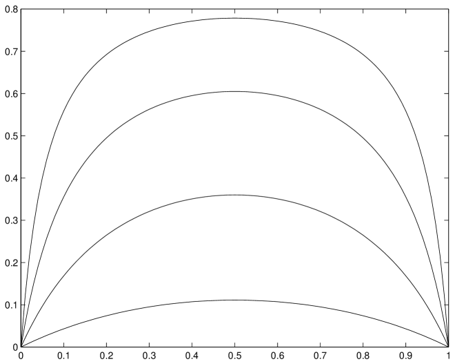
for any W𝑊W, where p𝑝p defines the attractor, see (15), and ρ=M/m𝜌𝑀𝑚\rho=M/m is the condition number of the operator. The function r(p)𝑟𝑝r(p) is symmetric with respect to 1/2121/2 and monotonously increasing from 0 to 1/2121/2, see Figure 2. The worst asymptotic rate is thus obtained at p=1/2𝑝12p=1/2:

Rmax=(ρ1ρ+1)2.subscript𝑅superscript𝜌1𝜌12R_{\max}=\left(\frac{\rho-1}{\rho+1}\right)^{2}\,. (23)
Refer to caption
Figure 2: r(p)𝑟𝑝r(p) as a function of p𝑝p, for ρ=2𝜌2\rho=2 (bottom curve), 4, 8 and 16 (top)

Note that kfor-all𝑘\forall k, rkRmaxsubscript𝑟𝑘subscript𝑅r_{k}\leq R_{\max} since rksubscript𝑟𝑘r_{k} is not decreasing, see Section 2.4. For a typical x0subscript𝑥0x_{0} (such that the convergence is not finite, that is, such that r(p)0𝑟𝑝0r(p)\neq 0), the stability analysis of Section 5 shows that only values of p𝑝p in ssubscript𝑠{\mathcal{I}}_{s} given by (21) may correspond to stable attractors. The range of possible values of R(p)𝑅𝑝R(p) is thus [Rmin,Rmax]subscript𝑅subscript𝑅[R_{\min},R_{\max}], where Rmaxsubscript𝑅R_{\max}, given by (23), is obtained for p=1/2𝑝12p=1/2 and

RminRmin=R(1/2+1/[22])=(ρ1)2(ρ+1)2+4ρ.subscript𝑅superscriptsubscript𝑅𝑅121delimited-[]22superscript𝜌12superscript𝜌124𝜌R_{\min}\leq R_{\min}^{*}=R(1/2+1/[2\sqrt{2}])=\frac{(\rho-1)^{2}}{(\rho+1)^{2}+4\rho}\,.

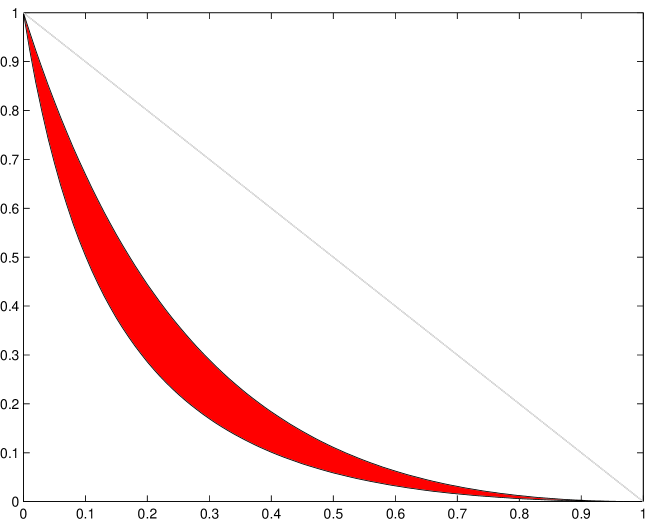
Figure 3 presents the range [Rmin,Rmax]superscriptsubscript𝑅subscript𝑅[R_{\min}^{*},R_{\max}] as a function of 1/ρ1𝜌1/\rho, the upper curve corresponding to Rmaxsubscript𝑅R_{\max} and the lower to Rminsuperscriptsubscript𝑅R_{\min}^{*}. The maximum size of the range is 3220.1716similar-to-or-equals3220.17163-2\sqrt{2}\simeq 0.1716, obtained at ρ=1+22+22+27.5239𝜌122222similar-to-or-equals7.5239\rho=1+2\sqrt{2}+2\sqrt{2+\sqrt{2}}\simeq 7.5239. These results confirm the experimental observation that the rate of convergence of the gradient algorithm is generally close to its worst value Rmaxsubscript𝑅R_{\max}, see NocedalSZ2002 . The same property is true for any P𝑃P-gradient algorithm.

Remark 2

A similar analysis for Dksubscript𝐷𝑘D_{k} defined by (12), which is also not decreasing, shows that DkD(p)=p(1p)(Mm)2subscript𝐷𝑘𝐷𝑝𝑝1𝑝superscript𝑀𝑚2D_{k}\rightarrow D(p)=p(1-p)(M-m)^{2} as k𝑘k\rightarrow\infty, with DkD=D(1/2)=(Mm)2/4subscript𝐷𝑘superscript𝐷𝐷12superscript𝑀𝑚24D_{k}\leq D^{*}=D(1/2)=(M-m)^{2}/4 for all k𝑘k. Also, for any typical x0subscript𝑥0x_{0} such that ps𝑝subscript𝑠p\in{\mathcal{I}}_{s} given by (21), we have D(p)D(1/2+1/[22])=(Mm)2/8𝐷𝑝𝐷121delimited-[]22superscript𝑀𝑚28D(p)\geq D(1/2+1/[2\sqrt{2}])=(M-m)^{2}/8.

Another quantity of interest is given by

ΔN=log(Rmax/Rmin)/[log(Rmax)log(Rmin)].subscriptΔ𝑁subscript𝑅subscript𝑅delimited-[]subscript𝑅subscript𝑅\Delta_{N}=\log(R_{\max}/R_{\min})/[\log(R_{\max})\log(R_{\min})]\,.

Indeed, for N𝑁N large enough, (WgN,gN)/(Wg0,g0)r(p)Nsimilar-to-or-equals𝑊subscript𝑔𝑁subscript𝑔𝑁𝑊subscript𝑔0subscript𝑔0𝑟superscript𝑝𝑁(Wg_{N},g_{N})/(Wg_{0},g_{0})\simeq r(p)^{N}, the number N𝑁N of iterations required for obtaining a ratio (WgN,gN)/(Wg0,g0)=ϵ𝑊subscript𝑔𝑁subscript𝑔𝑁𝑊subscript𝑔0subscript𝑔0italic-ϵ(Wg_{N},g_{N})/(Wg_{0},g_{0})=\epsilon (ϵ1)much-less-thanitalic-ϵ1(\epsilon\ll 1) is approximately log(ϵ)/log[r(p)]italic-ϵ𝑟𝑝\log(\epsilon)/\log[r(p)] and ΔN|log(ϵ)|subscriptΔ𝑁italic-ϵ\Delta_{N}|\log(\epsilon)| thus indicates the length of the interval of possible values for N𝑁N due to the range of possible values for p𝑝p. Direct calculation gives ΔN|log(Rmax)|<1/2subscriptΔ𝑁subscript𝑅12\Delta_{N}\,|\log(R_{\max})|<1/2 for any ρ𝜌\rho and

ΔN=ρ/81/4+𝒪(1/ρ), 1/log(Rmax)=ρ/4+𝒪(1/ρ)formulae-sequencesubscriptΔ𝑁𝜌814𝒪1𝜌1subscript𝑅𝜌4𝒪1𝜌\Delta_{N}=\rho/8-1/4+{\mathcal{O}}(1/\rho)\,,\ 1/\log(R_{\max})=-\rho/4+{\mathcal{O}}(1/\rho)

for large ρ𝜌\rho. Therefore, the number of iterations required by a P𝑃P-gradient algorithm to achieve a given precision ϵ<<1much-less-thanitalic-ϵ1\epsilon<<1 varies at most by a factor 2 depending on the (typical) starting point x0subscript𝑥0x_{0}, factors of variation close to 2 being possible only when ρ𝜌\rho is large.

The average value of R(W,x0,x)𝑅𝑊subscript𝑥0superscript𝑥R(W,x_{0},x^{*}) for z0=z(x0)subscript𝑧0𝑧subscript𝑥0z_{0}=z(x_{0}) uniformly distributed on the unit sphere is the same for any P𝑃P-gradient algorithm, more generally, the distribution of R(W,x0,x)𝑅𝑊subscript𝑥0superscript𝑥R(W,x_{0},x^{*}) associated with a particular distribution of z0subscript𝑧0z_{0} does not depend on the particular P𝑃P-gradient algorithm considered. Moreover, numerical simulations show that the average value of R(I,x0,x)𝑅𝐼subscript𝑥0superscript𝑥R(I,x_{0},x^{*}) is the same for the steepest-descent (P(A)=A1𝑃𝐴superscript𝐴1P(A)=A^{-1}) and minimum residues (P(A)=I𝑃𝐴𝐼P(A)=I) algorithms for x0subscript𝑥0x_{0} uniformly distributed on the sphere x0x=1normsubscript𝑥0superscript𝑥1\|x_{0}-x^{*}\|=1. The small deviations in average performance between different P𝑃P-gradient algorithms can only be related to the fact that a fixed distribution for x0subscript𝑥0x_{0} corresponds to different distributions for z(x0)𝑧subscript𝑥0z(x_{0}).

Refer to caption
Figure 3: Range [Rmin,Rmax]superscriptsubscript𝑅subscript𝑅[R_{\min}^{*},R_{\max}] of possible values of the asymptotic rate r(p)𝑟𝑝r(p) as a function of 1/ρ1𝜌1/\rho
Remark 3

It is known that the introduction of a relaxation coefficient γ𝛾\gamma, with 0<γ<10𝛾10<\gamma<1, in the steepest-descent algorithm totally changes its behaviour, see, e.g., Chapter 7 of PWZl2000 ; the algorithm (2) then becomes xk+1=xkγ[(gk,gk)/(Agk,gk)]gksubscript𝑥𝑘1subscript𝑥𝑘𝛾delimited-[]subscript𝑔𝑘subscript𝑔𝑘𝐴subscript𝑔𝑘subscript𝑔𝑘subscript𝑔𝑘x_{k+1}=x_{k}-\gamma[(g_{k},g_{k})/(Ag_{k},g_{k})]g_{k}. For =dsuperscript𝑑{\mathcal{H}}=\mathbb{R}^{d} and a fixed A𝐴A, depending on the value of γ𝛾\gamma, the renormalized process either converges to periodic orbits (the same for almost all starting points) or exhibits a chaotic behaviour, with the classical period-doubling phenomenon in the case d=2𝑑2d=2. In higher dimensions, repeated numerical trials show that the process typically no longer converges to the 2-dimensional plane spanned by (e1,ed)subscript𝑒1subscript𝑒𝑑(e_{1},e_{d}). A detailed analysis for d=2𝑑2d=2 and experimental results for d>2𝑑2d>2 also show that relaxation (with γ𝛾\gamma close to 1) considerably improves the rate of convergence. Similar results hold more generally for all P𝑃P-gradient algorithms, with the iteration (3) transformed into xk+1=xkγγkgksubscript𝑥𝑘1subscript𝑥𝑘𝛾subscript𝛾𝑘subscript𝑔𝑘x_{k+1}=x_{k}-\gamma\gamma_{k}g_{k}, with γ𝛾\gamma the (fixed) relaxation coefficient and γksubscript𝛾𝑘\gamma_{k} given by (4). Steepest descent with random relaxation coefficient γ(0,2)𝛾02\gamma\in(0,2) is considered in RaydanS2002 , avoiding the two point attraction and significantly improving the behavior of ordinary steepest descent.

Appendix

A1. Proof of Theorem 3.2. The proof relies on Theorem 4.2 (Theorem 4.1 when =dsuperscript𝑑{\mathcal{H}}=\mathbb{R}^{d}), which concerns successive transformations applied to a probability measure.

Since A𝐴A is self-adjoint, its spectrum SSAsubscriptSS𝐴\SS_{A} is a closed subset of the interval [m,M]𝑚𝑀[m,M] of the real line and m,MSSA𝑚𝑀subscriptSS𝐴m,M\in\SS_{A}. Let Eλsubscript𝐸𝜆E_{\lambda} be the spectral family associated with A𝐴A, and define the spectral measure νksubscript𝜈𝑘\nu_{k} by νk(dλ)=d(Eλzk,zk)subscript𝜈𝑘𝑑𝜆𝑑subscript𝐸𝜆subscript𝑧𝑘subscript𝑧𝑘\nu_{k}(d\lambda)=d(E_{\lambda}z_{k},z_{k}), mλM𝑚𝜆𝑀m\leq\lambda\leq M. Since (zk,zk)=mMνk(dλ)=1subscript𝑧𝑘subscript𝑧𝑘superscriptsubscript𝑚𝑀subscript𝜈𝑘𝑑𝜆1(z_{k},z_{k})=\int_{m}^{M}\nu_{k}(d\lambda)=1, νksubscript𝜈𝑘\nu_{k} is a probability measure on the Borel sets of (0,)0(0,\infty), with νk([m,M])=1subscript𝜈𝑘𝑚𝑀1\nu_{k}([m,M])=1 kfor-all𝑘\forall k. This representation gives

μ1=(Azk,zk)=λνk(dλ),μ2=(A2zk,zk)=λ2νk(dλ)formulae-sequencesubscript𝜇1𝐴subscript𝑧𝑘subscript𝑧𝑘𝜆subscript𝜈𝑘𝑑𝜆subscript𝜇2superscript𝐴2subscript𝑧𝑘subscript𝑧𝑘superscript𝜆2subscript𝜈𝑘𝑑𝜆\mu_{1}=(Az_{k},z_{k})=\int\lambda\,\nu_{k}(d\lambda)\,,\ \mu_{2}=(A^{2}z_{k},z_{k})=\int\lambda^{2}\,\nu_{k}(d\lambda)

where integration is over [m,M]𝑚𝑀[m,M] unless otherwise specified. Therefore, for any Borel set 𝒜𝒜{\mathcal{A}} the transformation (7) gives in terms of νksubscript𝜈𝑘\nu_{k}:

νk+1(𝒜)=𝒜[λλνk(dλ)]2νk(dλ)λ2νk(dλ)[λνk(dλ)]2.subscript𝜈𝑘1𝒜subscript𝒜superscriptdelimited-[]𝜆superscript𝜆subscript𝜈𝑘𝑑superscript𝜆2subscript𝜈𝑘𝑑𝜆superscript𝜆2subscript𝜈𝑘𝑑superscript𝜆superscriptdelimited-[]superscript𝜆subscript𝜈𝑘𝑑superscript𝜆2\nu_{k+1}({\mathcal{A}})=\frac{\int_{\mathcal{A}}\left[\lambda-\int\lambda^{\prime}\,\nu_{k}(d\lambda^{\prime})\right]^{2}\,\nu_{k}(d\lambda)}{\int\lambda^{\prime 2}\,\nu_{k}(d\lambda^{\prime})-\left[\int\lambda^{\prime}\,\nu_{k}(d\lambda^{\prime})\right]^{2}}\,.

The conditions (14) on z0subscript𝑧0z_{0} are equivalent to ess inf(ν0)=mess infsubscript𝜈0𝑚\mbox{\rm ess inf}(\nu_{0})=m and ess sup(ν0)=Mess supsubscript𝜈0𝑀\mbox{\rm ess sup}(\nu_{0})=M, see Theorem 4.2, and the updating rule for νksubscript𝜈𝑘\nu_{k} can be written as (18). Theorem 4.2 then implies (19), which can be written as: ϵ>0for-allitalic-ϵ0\forall\epsilon>0, ϵβ=(Mm)/2italic-ϵ𝛽𝑀𝑚2\epsilon\leq\beta=(M-m)/2,

(Em+ϵz2k,z2k)p,subscript𝐸𝑚italic-ϵsubscript𝑧2𝑘subscript𝑧2𝑘𝑝\displaystyle(E_{m+\epsilon}z_{2k},z_{2k})\rightarrow p\,, (EMϵz2k,z2k)p,subscript𝐸𝑀italic-ϵsubscript𝑧2𝑘subscript𝑧2𝑘𝑝\displaystyle(E_{M-\epsilon}z_{2k},z_{2k})\rightarrow p\,,
(Em+ϵz2k+1,z2k+1)1p,subscript𝐸𝑚italic-ϵsubscript𝑧2𝑘1subscript𝑧2𝑘11𝑝\displaystyle(E_{m+\epsilon}z_{2k+1},z_{2k+1})\rightarrow 1-p\,, (EMϵz2k+1,z2k+1)1p,subscript𝐸𝑀italic-ϵsubscript𝑧2𝑘1subscript𝑧2𝑘11𝑝\displaystyle(E_{M-\epsilon}z_{2k+1},z_{2k+1})\rightarrow 1-p\,,

as k𝑘k\rightarrow\infty, where p𝑝p depends on z0subscript𝑧0z_{0}, 0<p<10𝑝10<p<1. Define p2k=(Em+βz2k,z2k)subscript𝑝2𝑘subscript𝐸𝑚𝛽subscript𝑧2𝑘subscript𝑧2𝑘p_{2k}=(E_{m+\beta}z_{2k},z_{2k}), p2k+1=1(Em+βz2k+1,z2k+1)subscript𝑝2𝑘11subscript𝐸𝑚𝛽subscript𝑧2𝑘1subscript𝑧2𝑘1p_{2k+1}=1-(E_{m+\beta}z_{2k+1},z_{2k+1}), and the angles φ𝜑\varphi, φnsubscript𝜑𝑛\varphi_{n} by cosφ=p𝜑𝑝\cos\varphi=\sqrt{p}, sinφ=1p𝜑1𝑝\sin\varphi=\sqrt{1-p}, cosφn=pnsubscript𝜑𝑛subscript𝑝𝑛\cos\varphi_{n}=\sqrt{p_{n}}, sinφn=1pnsubscript𝜑𝑛1subscript𝑝𝑛\sin\varphi_{n}=\sqrt{1-p_{n}}, nfor-all𝑛\forall n. Also define s2k=Em+βz2k/cosφ2ksubscript𝑠2𝑘subscript𝐸𝑚𝛽subscript𝑧2𝑘subscript𝜑2𝑘s_{2k}=E_{m+\beta}z_{2k}/\cos\varphi_{2k}, s2k+1=Em+βz2k+1/sinφ2k+1subscript𝑠2𝑘1subscript𝐸𝑚𝛽subscript𝑧2𝑘1subscript𝜑2𝑘1s_{2k+1}=E_{m+\beta}z_{2k+1}/\sin\varphi_{2k+1}, t2k=(z2kEm+βz2k)/sinφ2ksubscript𝑡2𝑘subscript𝑧2𝑘subscript𝐸𝑚𝛽subscript𝑧2𝑘subscript𝜑2𝑘t_{2k}=(z_{2k}-E_{m+\beta}z_{2k})/\sin\varphi_{2k}, t2k+1=(z2k+1Em+βz2k+1)/cosφ2k+1subscript𝑡2𝑘1subscript𝑧2𝑘1subscript𝐸𝑚𝛽subscript𝑧2𝑘1subscript𝜑2𝑘1t_{2k+1}=-(z_{2k+1}-E_{m+\beta}z_{2k+1})/\cos\varphi_{2k+1}. This gives pnpsubscript𝑝𝑛𝑝p_{n}\rightarrow p as n𝑛n\rightarrow\infty, sn=tn=1normsubscript𝑠𝑛normsubscript𝑡𝑛1\|s_{n}\|=\|t_{n}\|=1 nfor-all𝑛\forall n, and z2k=cosφ2ks2k+sinφ2kt2ksubscript𝑧2𝑘subscript𝜑2𝑘subscript𝑠2𝑘subscript𝜑2𝑘subscript𝑡2𝑘z_{2k}=\cos\varphi_{2k}\,s_{2k}+\sin\varphi_{2k}\,t_{2k}, z2k+1=sinφ2k+1s2k+1cosφ2k+1t2k+1subscript𝑧2𝑘1subscript𝜑2𝑘1subscript𝑠2𝑘1subscript𝜑2𝑘1subscript𝑡2𝑘1z_{2k+1}=\sin\varphi_{2k+1}\,s_{2k+1}-\cos\varphi_{2k+1}\,t_{2k+1}. Also,

Asnmsn2=(λm)2d(Eλsn,sn),superscriptnorm𝐴subscript𝑠𝑛𝑚subscript𝑠𝑛2superscript𝜆𝑚2𝑑subscript𝐸𝜆subscript𝑠𝑛subscript𝑠𝑛\|As_{n}-ms_{n}\|^{2}=\int(\lambda-m)^{2}\,d(E_{\lambda}s_{n},s_{n})\,,

which, for n=2k𝑛2𝑘n=2k and any ϵitalic-ϵ\epsilon, 0<ϵ<β0italic-ϵ𝛽0<\epsilon<\beta, gives

As2kms2k2superscriptnorm𝐴subscript𝑠2𝑘𝑚subscript𝑠2𝑘2\displaystyle\|As_{2k}-ms_{2k}\|^{2} =\displaystyle= mm+β(λm)2p2kd(Eλz2k,z2k)superscriptsubscript𝑚𝑚𝛽superscript𝜆𝑚2subscript𝑝2𝑘𝑑subscript𝐸𝜆subscript𝑧2𝑘subscript𝑧2𝑘\displaystyle\int_{m}^{m+\beta}\frac{(\lambda-m)^{2}}{p_{2k}}\,d(E_{\lambda}z_{2k},z_{2k})
=\displaystyle= mm+ϵ(λm)2p2kd(Eλz2k,z2k)+m+ϵm+β(λm)2p2kd(Eλz2k,z2k)superscriptsubscript𝑚𝑚italic-ϵsuperscript𝜆𝑚2subscript𝑝2𝑘𝑑subscript𝐸𝜆subscript𝑧2𝑘subscript𝑧2𝑘superscriptsubscript𝑚italic-ϵ𝑚𝛽superscript𝜆𝑚2subscript𝑝2𝑘𝑑subscript𝐸𝜆subscript𝑧2𝑘subscript𝑧2𝑘\displaystyle\int_{m}^{m+\epsilon}\frac{(\lambda-m)^{2}}{p_{2k}}\,d(E_{\lambda}z_{2k},z_{2k})+\int_{m+\epsilon}^{m+\beta}\frac{(\lambda-m)^{2}}{p_{2k}}\,d(E_{\lambda}z_{2k},z_{2k})
ϵ2p2k+β2p2k[p2kmm+ϵd(Eλz2k,z2k)].absentsuperscriptitalic-ϵ2subscript𝑝2𝑘superscript𝛽2subscript𝑝2𝑘delimited-[]subscript𝑝2𝑘superscriptsubscript𝑚𝑚italic-ϵ𝑑subscript𝐸𝜆subscript𝑧2𝑘subscript𝑧2𝑘\displaystyle\leq\frac{\epsilon^{2}}{p_{2k}}+\frac{\beta^{2}}{p_{2k}}\left[p_{2k}-\int_{m}^{m+\epsilon}d(E_{\lambda}z_{2k},z_{2k})\right]\,.

Since p2kpsubscript𝑝2𝑘𝑝p_{2k}\rightarrow p and mm+ϵd(Eλz2k,z2k)psuperscriptsubscript𝑚𝑚italic-ϵ𝑑subscript𝐸𝜆subscript𝑧2𝑘subscript𝑧2𝑘𝑝\int_{m}^{m+\epsilon}d(E_{\lambda}z_{2k},z_{2k})\rightarrow p as k𝑘k\rightarrow\infty, As2kms2k0norm𝐴subscript𝑠2𝑘𝑚subscript𝑠2𝑘0\|As_{2k}-ms_{2k}\|\rightarrow 0 as k𝑘k\rightarrow\infty. Similarly, As2k+1ms2k+10norm𝐴subscript𝑠2𝑘1𝑚subscript𝑠2𝑘10\|As_{2k+1}-ms_{2k+1}\|\rightarrow 0 as k𝑘k\rightarrow\infty and AtnMtn0norm𝐴subscript𝑡𝑛𝑀subscript𝑡𝑛0\|At_{n}-Mt_{n}\|\rightarrow 0 as n𝑛n\rightarrow\infty. Consider now

un=cosϑnsn+sinϑntn,vn=sinϑnsn+cosϑntn.formulae-sequencesubscript𝑢𝑛subscriptitalic-ϑ𝑛subscript𝑠𝑛subscriptitalic-ϑ𝑛subscript𝑡𝑛subscript𝑣𝑛subscriptitalic-ϑ𝑛subscript𝑠𝑛subscriptitalic-ϑ𝑛subscript𝑡𝑛u_{n}=\cos\vartheta_{n}\,s_{n}+\sin\vartheta_{n}\,t_{n}\,,\ v_{n}=-\sin\vartheta_{n}\,s_{n}+\cos\vartheta_{n}\,t_{n}\,.

Straightforward calculations show that ϑn=φnφsubscriptitalic-ϑ𝑛subscript𝜑𝑛𝜑\vartheta_{n}=\varphi_{n}-\varphi gives (15) with un=vn=1normsubscript𝑢𝑛normsubscript𝑣𝑛1\|u_{n}\|=\|v_{n}\|=1 nfor-all𝑛\forall n. Also

Aunmun|cosϑn|Asnmsn+|sinϑn|(Mm),norm𝐴subscript𝑢𝑛𝑚subscript𝑢𝑛subscriptitalic-ϑ𝑛norm𝐴subscript𝑠𝑛𝑚subscript𝑠𝑛subscriptitalic-ϑ𝑛𝑀𝑚\|Au_{n}-mu_{n}\|\leq|\cos\vartheta_{n}|\|As_{n}-ms_{n}\|+|\sin\vartheta_{n}|(M-m)\,,

and, since Asnmsn0norm𝐴subscript𝑠𝑛𝑚subscript𝑠𝑛0\|As_{n}-ms_{n}\|\rightarrow 0, ϑn0subscriptitalic-ϑ𝑛0\vartheta_{n}\rightarrow 0 as n𝑛n\rightarrow\infty, Aunmun0norm𝐴subscript𝑢𝑛𝑚subscript𝑢𝑛0\|Au_{n}-mu_{n}\|\rightarrow 0 as n𝑛n\rightarrow\infty. Similarly, AvnMvn0norm𝐴subscript𝑣𝑛𝑀subscript𝑣𝑛0\|Av_{n}-Mv_{n}\|\rightarrow 0 as n𝑛n\rightarrow\infty.  

A2. Proof of Theorem 4.1. We first prove that the mass of νksubscript𝜈𝑘\nu_{k} tends to concentrate on two eigenvalues only. When ν0subscript𝜈0\nu_{0} is non degenerate, L1>1subscript𝐿11L_{1}>1 from Jensen inequality, and thus, since (Lk)subscript𝐿𝑘(L_{k}) is non-decreasing, see Section 2.4, LkL1>1subscript𝐿𝑘subscript𝐿11L_{k}\geq L_{1}>1. Now, from Lagrange identity (ai2)(bi2)=i<j(aibjajbi)2+(aibi)2superscriptsubscript𝑎𝑖2superscriptsubscript𝑏𝑖2subscript𝑖𝑗superscriptsubscript𝑎𝑖subscript𝑏𝑗subscript𝑎𝑗subscript𝑏𝑖2superscriptsubscript𝑎𝑖subscript𝑏𝑖2(\sum a_{i}^{2})(\sum b_{i}^{2})=\sum_{i<j}(a_{i}b_{j}-a_{j}b_{i})^{2}+(\sum a_{i}b_{i})^{2}

Lksubscript𝐿𝑘\displaystyle L_{k} =\displaystyle= (i=1dλi[zk]i2)(i=1d[zk]i2/λi)superscriptsubscript𝑖1𝑑subscript𝜆𝑖superscriptsubscriptdelimited-[]subscript𝑧𝑘𝑖2superscriptsubscript𝑖1𝑑superscriptsubscriptdelimited-[]subscript𝑧𝑘𝑖2subscript𝜆𝑖\displaystyle\left(\sum_{i=1}^{d}\lambda_{i}[z_{k}]_{i}^{2}\right)\,\left(\sum_{i=1}^{d}[z_{k}]_{i}^{2}/\lambda_{i}\right)
=\displaystyle= i<j[zk]i2[zk]j2(λiλjλjλi)2+(i=1d[zk]i2)2subscript𝑖𝑗superscriptsubscriptdelimited-[]subscript𝑧𝑘𝑖2superscriptsubscriptdelimited-[]subscript𝑧𝑘𝑗2superscriptsubscript𝜆𝑖subscript𝜆𝑗subscript𝜆𝑗subscript𝜆𝑖2superscriptsuperscriptsubscript𝑖1𝑑superscriptsubscriptdelimited-[]subscript𝑧𝑘𝑖22\displaystyle\sum_{i<j}[z_{k}]_{i}^{2}[z_{k}]_{j}^{2}\left(\frac{\sqrt{\lambda_{i}}}{\sqrt{\lambda_{j}}}-\frac{\sqrt{\lambda_{j}}}{\sqrt{\lambda_{i}}}\right)^{2}+\left(\sum_{i=1}^{d}[z_{k}]_{i}^{2}\right)^{2}
=\displaystyle= i<j[zk]i2[zk]j2(λiλj)2λiλj+1.subscript𝑖𝑗superscriptsubscriptdelimited-[]subscript𝑧𝑘𝑖2superscriptsubscriptdelimited-[]subscript𝑧𝑘𝑗2superscriptsubscript𝜆𝑖subscript𝜆𝑗2subscript𝜆𝑖subscript𝜆𝑗1\displaystyle\sum_{i<j}[z_{k}]_{i}^{2}[z_{k}]_{j}^{2}\frac{(\lambda_{i}-\lambda_{j})^{2}}{\lambda_{i}\lambda_{j}}+1\,.

Let iksubscript𝑖𝑘i_{k} and jksubscript𝑗𝑘j_{k} denote the indices that achieve maxi<j[zk]i2[zk]j2\max_{i<j}[z_{k}]_{i}^{2}[z_{k}]_{j}^{2}. We have

Lk[zk]ik2[zk]jk2i<j(λiλj)2λiλj+1subscript𝐿𝑘superscriptsubscriptdelimited-[]subscript𝑧𝑘subscript𝑖𝑘2superscriptsubscriptdelimited-[]subscript𝑧𝑘subscript𝑗𝑘2subscript𝑖𝑗superscriptsubscript𝜆𝑖subscript𝜆𝑗2subscript𝜆𝑖subscript𝜆𝑗1L_{k}\leq[z_{k}]_{i_{k}}^{2}[z_{k}]_{j_{k}}^{2}\sum_{i<j}\frac{(\lambda_{i}-\lambda_{j})^{2}}{\lambda_{i}\lambda_{j}}+1

and thus

[zk]ik2[zk]jk2δ=L11i<j(λiλj)2λiλj.superscriptsubscriptdelimited-[]subscript𝑧𝑘subscript𝑖𝑘2superscriptsubscriptdelimited-[]subscript𝑧𝑘subscript𝑗𝑘2𝛿subscript𝐿11subscript𝑖𝑗superscriptsubscript𝜆𝑖subscript𝜆𝑗2subscript𝜆𝑖subscript𝜆𝑗[z_{k}]_{i_{k}}^{2}[z_{k}]_{j_{k}}^{2}\geq\delta=\frac{L_{1}-1}{\sum_{i<j}\frac{(\lambda_{i}-\lambda_{j})^{2}}{\lambda_{i}\lambda_{j}}}\,.

Moreover, [zk]ik2+[zk]jk2<1superscriptsubscriptdelimited-[]subscript𝑧𝑘subscript𝑖𝑘2superscriptsubscriptdelimited-[]subscript𝑧𝑘subscript𝑗𝑘21[z_{k}]_{i_{k}}^{2}+[z_{k}]_{j_{k}}^{2}<1 gives

δ<[zk]ik2<1δ and δ<[zk]jk2<1δ.𝛿superscriptsubscriptdelimited-[]subscript𝑧𝑘subscript𝑖𝑘21𝛿 and 𝛿superscriptsubscriptdelimited-[]subscript𝑧𝑘subscript𝑗𝑘21𝛿\delta<[z_{k}]_{i_{k}}^{2}<1-\delta\ \mbox{ and }\ \delta<[z_{k}]_{j_{k}}^{2}<1-\delta\,.

Consider the matrix 𝐌ksubscript𝐌𝑘{\bf M}_{k} given by (10). Its determinant can be written as

det𝐌ksubscript𝐌𝑘\displaystyle\det{\bf M}_{k} =\displaystyle= i<j<l[zk]i2[zk]j2[zk]l2(λiλj)2(λiλl)2(λjλl)2λiλjλlsubscript𝑖𝑗𝑙superscriptsubscriptdelimited-[]subscript𝑧𝑘𝑖2superscriptsubscriptdelimited-[]subscript𝑧𝑘𝑗2superscriptsubscriptdelimited-[]subscript𝑧𝑘𝑙2superscriptsubscript𝜆𝑖subscript𝜆𝑗2superscriptsubscript𝜆𝑖subscript𝜆𝑙2superscriptsubscript𝜆𝑗subscript𝜆𝑙2subscript𝜆𝑖subscript𝜆𝑗subscript𝜆𝑙\displaystyle\sum_{i<j<l}[z_{k}]_{i}^{2}[z_{k}]_{j}^{2}[z_{k}]_{l}^{2}\frac{(\lambda_{i}-\lambda_{j})^{2}(\lambda_{i}-\lambda_{l})^{2}(\lambda_{j}-\lambda_{l})^{2}}{\lambda_{i}\lambda_{j}\lambda_{l}}
[zk]ik2[zk]jk2(λikλjk)2iik,jk[zk]i2(λiλik)2(λiλjk)2λiλikλjkabsentsuperscriptsubscriptdelimited-[]subscript𝑧𝑘subscript𝑖𝑘2superscriptsubscriptdelimited-[]subscript𝑧𝑘subscript𝑗𝑘2superscriptsubscript𝜆subscript𝑖𝑘subscript𝜆subscript𝑗𝑘2subscript𝑖subscript𝑖𝑘subscript𝑗𝑘superscriptsubscriptdelimited-[]subscript𝑧𝑘𝑖2superscriptsubscript𝜆𝑖subscript𝜆subscript𝑖𝑘2superscriptsubscript𝜆𝑖subscript𝜆subscript𝑗𝑘2subscript𝜆𝑖subscript𝜆subscript𝑖𝑘subscript𝜆subscript𝑗𝑘\displaystyle\geq[z_{k}]_{i_{k}}^{2}[z_{k}]_{j_{k}}^{2}(\lambda_{i_{k}}-\lambda_{j_{k}})^{2}\sum_{i\neq i_{k},j_{k}}[z_{k}]_{i}^{2}\frac{(\lambda_{i}-\lambda_{i_{k}})^{2}(\lambda_{i}-\lambda_{j_{k}})^{2}}{\lambda_{i}\lambda_{i_{k}}\lambda_{j_{k}}}
δδλ6M3iik,jk[zk]i2absent𝛿superscriptsubscript𝛿𝜆6superscript𝑀3subscript𝑖subscript𝑖𝑘subscript𝑗𝑘superscriptsubscriptdelimited-[]subscript𝑧𝑘𝑖2\displaystyle\geq\delta\frac{\delta_{\lambda}^{6}}{M^{3}}\sum_{i\neq i_{k},j_{k}}[z_{k}]_{i}^{2}

where

δλ=mini,j|λiλj|.subscript𝛿𝜆subscript𝑖𝑗subscript𝜆𝑖subscript𝜆𝑗\delta_{\lambda}=\min_{i,j}|\lambda_{i}-\lambda_{j}|\,.

Since det𝐌k0subscript𝐌𝑘0\det{\bf M}_{k}\rightarrow 0 as k𝑘k\rightarrow\infty, see (11), we get iik,jk[zk]i20subscript𝑖subscript𝑖𝑘subscript𝑗𝑘superscriptsubscriptdelimited-[]subscript𝑧𝑘𝑖20\sum_{i\neq i_{k},j_{k}}[z_{k}]_{i}^{2}\rightarrow 0 as k𝑘k\rightarrow\infty. The mass thus tends to concentrate on λik,λjksubscript𝜆subscript𝑖𝑘subscript𝜆subscript𝑗𝑘\lambda_{i_{k}},\lambda_{j_{k}}.

Next we prove that iksubscript𝑖𝑘i_{k} and jksubscript𝑗𝑘j_{k} eventually become fixed. From the result above, ϵ>0for-allitalic-ϵ0\forall\epsilon>0, kϵsubscript𝑘italic-ϵ\exists k_{\epsilon} such that iik,jk[zk]i2<ϵsubscript𝑖subscript𝑖𝑘subscript𝑗𝑘superscriptsubscriptdelimited-[]subscript𝑧𝑘𝑖2italic-ϵ\sum_{i\neq i_{k},j_{k}}[z_{k}]_{i}^{2}<\epsilon, k>kϵ𝑘subscript𝑘italic-ϵk>k_{\epsilon}.

Consider the updating equation (16). We have for any i𝑖i, (μ1kλi)2(Mm)2superscriptsuperscriptsubscript𝜇1𝑘subscript𝜆𝑖2superscript𝑀𝑚2(\mu_{1}^{k}-\lambda_{i})^{2}\leq(M-m)^{2}. Also, Dk=μ2k(μ1k)2D0subscript𝐷𝑘superscriptsubscript𝜇2𝑘superscriptsuperscriptsubscript𝜇1𝑘2subscript𝐷0D_{k}=\mu_{2}^{k}-(\mu_{1}^{k})^{2}\geq D_{0}, see Section 2.4. This gives for iik,jk𝑖subscript𝑖𝑘subscript𝑗𝑘i\neq i_{k},j_{k} and k>kϵ𝑘subscript𝑘italic-ϵk>k_{\epsilon}

[zk+1]i2<ϵ(Mm)2D0.superscriptsubscriptdelimited-[]subscript𝑧𝑘1𝑖2italic-ϵsuperscript𝑀𝑚2subscript𝐷0[z_{k+1}]_{i}^{2}<\epsilon\frac{(M-m)^{2}}{D_{0}}\,.

Taking ϵ1=δD0/(Mm)2subscriptitalic-ϵ1𝛿subscript𝐷0superscript𝑀𝑚2\epsilon_{1}=\delta D_{0}/(M-m)^{2} we obtain [zk+1]i2<δsuperscriptsubscriptdelimited-[]subscript𝑧𝑘1𝑖2𝛿[z_{k+1}]_{i}^{2}<\delta for iik,jk𝑖subscript𝑖𝑘subscript𝑗𝑘i\neq i_{k},j_{k} and k>kϵ1𝑘subscript𝑘subscriptitalic-ϵ1k>k_{\epsilon_{1}}. Since [zk+1]ik+12>δsuperscriptsubscriptdelimited-[]subscript𝑧𝑘1subscript𝑖𝑘12𝛿[z_{k+1}]_{i_{k+1}}^{2}>\delta and [zk+1]jk+12>δsuperscriptsubscriptdelimited-[]subscript𝑧𝑘1subscript𝑗𝑘12𝛿[z_{k+1}]_{j_{k+1}}^{2}>\delta, i{ik,jk}𝑖subscript𝑖𝑘subscript𝑗𝑘i\not\in\{i_{k},j_{k}\} implies i{ik+1,jk+1}𝑖subscript𝑖𝑘1subscript𝑗𝑘1i\not\in\{i_{k+1},j_{k+1}\}, k>kϵ1𝑘subscript𝑘subscriptitalic-ϵ1k>k_{\epsilon_{1}} and thus {ik,jk}={i,j}subscript𝑖𝑘subscript𝑗𝑘superscript𝑖superscript𝑗\{i_{k},j_{k}\}=\{i^{*},j^{*}\} for k>kϵ1𝑘subscript𝑘subscriptitalic-ϵ1k>k_{\epsilon_{1}}.

We show now that {i,j}={1,d}superscript𝑖superscript𝑗1𝑑\{i^{*},j^{*}\}=\{1,d\}. Assume that i<j<dsuperscript𝑖superscript𝑗𝑑i^{*}<j^{*}<d (which implies [zk]d20superscriptsubscriptdelimited-[]subscript𝑧𝑘𝑑20[z_{k}]_{d}^{2}\rightarrow 0, k𝑘k\rightarrow\infty). We need to show that (λdμ1k)2>(λjμ1k)2superscriptsubscript𝜆𝑑superscriptsubscript𝜇1𝑘2superscriptsubscript𝜆superscript𝑗superscriptsubscript𝜇1𝑘2(\lambda_{d}-\mu_{1}^{k})^{2}>(\lambda_{j^{*}}-\mu_{1}^{k})^{2} for k𝑘k large enough. We have

μ1k=λi[zk]i2+λj[zk]j2+ii,jλi[zk]i2λi[zk]i2+λj[zk]j2+λdii,j[zk]i2.superscriptsubscript𝜇1𝑘subscript𝜆superscript𝑖superscriptsubscriptdelimited-[]subscript𝑧𝑘superscript𝑖2subscript𝜆superscript𝑗superscriptsubscriptdelimited-[]subscript𝑧𝑘superscript𝑗2subscript𝑖superscript𝑖superscript𝑗subscript𝜆𝑖superscriptsubscriptdelimited-[]subscript𝑧𝑘𝑖2subscript𝜆superscript𝑖superscriptsubscriptdelimited-[]subscript𝑧𝑘superscript𝑖2subscript𝜆superscript𝑗superscriptsubscriptdelimited-[]subscript𝑧𝑘superscript𝑗2subscript𝜆𝑑subscript𝑖superscript𝑖superscript𝑗superscriptsubscriptdelimited-[]subscript𝑧𝑘𝑖2\mu_{1}^{k}=\lambda_{i^{*}}[z_{k}]_{i^{*}}^{2}+\lambda_{j^{*}}[z_{k}]_{j^{*}}^{2}+\sum_{i\neq i^{*},j^{*}}\lambda_{i}[z_{k}]_{i}^{2}\leq\lambda_{i^{*}}[z_{k}]_{i^{*}}^{2}+\lambda_{j^{*}}[z_{k}]_{j^{*}}^{2}+\lambda_{d}\sum_{i\neq i^{*},j^{*}}[z_{k}]_{i}^{2}\,.

Take ϵ2=min{ϵ1,δδλ/λd}subscriptitalic-ϵ2subscriptitalic-ϵ1𝛿subscript𝛿𝜆subscript𝜆𝑑\epsilon_{2}=\min\{\epsilon_{1},\delta\delta_{\lambda}/\lambda_{d}\}. For k>kϵ2𝑘subscript𝑘subscriptitalic-ϵ2k>k_{\epsilon_{2}} we have

μ1kλi[zk]i2+λj[zk]j2+λdϵ2λiδ+λj(1δ)+λdϵ2λjδδλ+λdϵ2λjsuperscriptsubscript𝜇1𝑘subscript𝜆superscript𝑖superscriptsubscriptdelimited-[]subscript𝑧𝑘superscript𝑖2subscript𝜆superscript𝑗superscriptsubscriptdelimited-[]subscript𝑧𝑘superscript𝑗2subscript𝜆𝑑subscriptitalic-ϵ2subscript𝜆superscript𝑖𝛿subscript𝜆superscript𝑗1𝛿subscript𝜆𝑑subscriptitalic-ϵ2subscript𝜆superscript𝑗𝛿subscript𝛿𝜆subscript𝜆𝑑subscriptitalic-ϵ2subscript𝜆superscript𝑗\mu_{1}^{k}\leq\lambda_{i^{*}}[z_{k}]_{i^{*}}^{2}+\lambda_{j^{*}}[z_{k}]_{j^{*}}^{2}+\lambda_{d}\epsilon_{2}\leq\lambda_{i^{*}}\delta+\lambda_{j^{*}}(1-\delta)+\lambda_{d}\epsilon_{2}\leq\lambda_{j^{*}}-\delta\delta_{\lambda}+\lambda_{d}\epsilon_{2}\leq\lambda_{j^{*}}

and thus (λdμ1k)2>(λjμ1k)2superscriptsubscript𝜆𝑑superscriptsubscript𝜇1𝑘2superscriptsubscript𝜆superscript𝑗superscriptsubscript𝜇1𝑘2(\lambda_{d}-\mu_{1}^{k})^{2}>(\lambda_{j^{*}}-\mu_{1}^{k})^{2}. From (16), this gives for k>kϵ2𝑘subscript𝑘subscriptitalic-ϵ2k>k_{\epsilon_{2}}

([zk+1]d[zk]d)2=(λdμ1k)2Dk>(λjμ1k)2Dk=([zk+1]j[zk]j)2superscriptsubscriptdelimited-[]subscript𝑧𝑘1𝑑subscriptdelimited-[]subscript𝑧𝑘𝑑2superscriptsubscript𝜆𝑑superscriptsubscript𝜇1𝑘2subscript𝐷𝑘superscriptsubscript𝜆superscript𝑗superscriptsubscript𝜇1𝑘2subscript𝐷𝑘superscriptsubscriptdelimited-[]subscript𝑧𝑘1superscript𝑗subscriptdelimited-[]subscript𝑧𝑘superscript𝑗2\left(\frac{[z_{k+1}]_{d}}{[z_{k}]_{d}}\right)^{2}=\frac{(\lambda_{d}-\mu_{1}^{k})^{2}}{D_{k}}>\frac{(\lambda_{j^{*}}-\mu_{1}^{k})^{2}}{D_{k}}=\left(\frac{[z_{k+1}]_{j^{*}}}{[z_{k}]_{j^{*}}}\right)^{2}

and thus

([zk+1]j[zk+1]d)2<([zk]j[zk]d)2.superscriptsubscriptdelimited-[]subscript𝑧𝑘1superscript𝑗subscriptdelimited-[]subscript𝑧𝑘1𝑑2superscriptsubscriptdelimited-[]subscript𝑧𝑘superscript𝑗subscriptdelimited-[]subscript𝑧𝑘𝑑2\left(\frac{[z_{k+1}]_{j^{*}}}{[z_{k+1}]_{d}}\right)^{2}<\left(\frac{[z_{k}]_{j^{*}}}{[z_{k}]_{d}}\right)^{2}\,.

We arrived at a contradiction since [zk]d20superscriptsubscriptdelimited-[]subscript𝑧𝑘𝑑20[z_{k}]_{d}^{2}\rightarrow 0 and [zk]j2superscriptsubscriptdelimited-[]subscript𝑧𝑘superscript𝑗2[z_{k}]_{j^{*}}^{2} is bounded from below by δ𝛿\delta. Therefore j=dsuperscript𝑗𝑑j^{*}=d. Similarly, i=1superscript𝑖1i^{*}=1.

Finally, let L𝐿L denote limkLksubscript𝑘subscript𝐿𝑘\lim_{k\rightarrow\infty}L_{k}, see Section 2.4. There are only two discrete measures with nonzero masses on λ1subscript𝜆1\lambda_{1} and λdsubscript𝜆𝑑\lambda_{d} and such that μ1μ1=Lsubscript𝜇1subscript𝜇1𝐿\mu_{1}\mu_{-1}=L,

ν(1)={λ1λdp1p} and ν(2)={λ1λd1pp}superscript𝜈1subscript𝜆1subscript𝜆𝑑𝑝1𝑝 and superscript𝜈2subscript𝜆1subscript𝜆𝑑1𝑝𝑝\nu^{(1)}=\left\{\begin{array}[]{cc}\lambda_{1}&\lambda_{d}\\ p&1-p\end{array}\right\}\ \mbox{ and }\ \nu^{(2)}=\left\{\begin{array}[]{cc}\lambda_{1}&\lambda_{d}\\ 1-p&p\end{array}\right\}

with

p=12ρ+1ρ114ρL(ρ+1)2𝑝12𝜌1𝜌114𝜌𝐿superscript𝜌12p=\frac{1}{2}-\frac{\rho+1}{\rho-1}\sqrt{\frac{1}{4}-\frac{\rho L}{(\rho+1)^{2}}}

and ρ=M/m𝜌𝑀𝑚\rho=M/m. Direct calculation shows that νk=ν(1)subscript𝜈𝑘superscript𝜈1\nu_{k}=\nu^{(1)} gives νk+1=ν(2)subscript𝜈𝑘1superscript𝜈2\nu_{k+1}=\nu^{(2)}, hence the convergence of νksubscript𝜈𝑘\nu_{k} to the cyclic attractor ν(1)ν(2)ν(1)superscript𝜈1superscript𝜈2superscript𝜈1\nu^{(1)}\rightarrow\nu^{(2)}\rightarrow\nu^{(1)}\rightarrow\cdots  

A3. The proof of Theorem 4.2 is more technical than that of Theorem 4.1 and relies on a series of lemmas stated below.

Lemma 1

Let ν𝜈\nu be any probability distribution on [m,M]𝑚𝑀[m,M], 0<mM<0𝑚𝑀0<m\leq M<\infty with moments μi=λiν(dλ)subscript𝜇𝑖superscript𝜆𝑖𝜈𝑑𝜆\mu_{i}=\int\lambda^{i}\nu(d\lambda), i𝑖i\in\mathbb{Z} (μ0=1subscript𝜇01\mu_{0}=1). Then,

μ2μ12subscript𝜇2superscriptsubscript𝜇12\displaystyle\mu_{2}-\mu_{1}^{2} \displaystyle\leq D=(Mm)2/4superscript𝐷superscript𝑀𝑚24\displaystyle D^{*}=(M-m)^{2}/4 (24)
μ1μ1subscript𝜇1subscript𝜇1\displaystyle\mu_{1}\mu_{-1} \displaystyle\leq L=(M+m)2/(4mM).superscript𝐿superscript𝑀𝑚24𝑚𝑀\displaystyle L^{*}=(M+m)^{2}/(4mM)\,. (25)

Proof. The proof relies on standard results in experimental design theory, see, e.g., Fedorov72 ; Silvey80 . Consider the two linear regression models η1(θ,λ)=θ0+θ1λsubscript𝜂1𝜃𝜆subscript𝜃0subscript𝜃1𝜆\eta_{1}(\theta,\lambda)=\theta_{0}+\theta_{1}\lambda and η2(θ,λ)=θ0/λ+θ1λsubscript𝜂2𝜃𝜆subscript𝜃0𝜆subscript𝜃1𝜆\eta_{2}(\theta,\lambda)=\theta_{0}/\sqrt{\lambda}+\theta_{1}\sqrt{\lambda}, with θ0,θ1subscript𝜃0subscript𝜃1\theta_{0},\theta_{1} the model parameters and λ𝜆\lambda the design variable, λ[m,M]𝜆𝑚𝑀\lambda\in[m,M]. D𝐷D-optimum design (approximate theory) aims at determining a probability measure on [m,M]𝑚𝑀[m,M] that maximizes the determinant of the information matrix associated with a particular model, here respectively

𝐈1(ν)=(μ0μ1μ1μ2) and 𝐈2(ν)=(μ1μ0μ0μ1).subscript𝐈1𝜈subscript𝜇0subscript𝜇1subscript𝜇1subscript𝜇2 and subscript𝐈2𝜈subscript𝜇1subscript𝜇0subscript𝜇0subscript𝜇1{\bf I}_{1}(\nu)=\left(\begin{array}[]{cc}\mu_{0}&\mu_{1}\\ \mu_{1}&\mu_{2}\end{array}\right)\ \mbox{ and }\ {\bf I}_{2}(\nu)=\left(\begin{array}[]{cc}\mu_{-1}&\mu_{0}\\ \mu_{0}&\mu_{1}\end{array}\right)\,.

The function logdet𝐈(ν)𝐈𝜈\log\det{\bf I}(\nu) is concave on the set of probability measures on [m,M]𝑚𝑀[m,M], and its maximum is unique. The Kiefer-Wolfowitz General Equivalence Theorem KieferW60 gives a characterization of the measure νsuperscript𝜈\nu^{*} that maximizes det𝐈1(ν)=μ2μ12subscript𝐈1𝜈subscript𝜇2superscriptsubscript𝜇12\det{\bf I}_{1}(\nu)=\mu_{2}-\mu_{1}^{2} and det𝐈2(ν)=μ1μ11subscript𝐈2𝜈subscript𝜇1subscript𝜇11\det{\bf I}_{2}(\nu)=\mu_{1}\mu_{-1}-1. In this case it corresponds to the two point measure, supported at m𝑚m and M𝑀M, with both masses equal to 1/2121/2. Direct calculation gives (24,25). One may notice that (25) corresponds to the Kantorovich inequality, see KantorovichA82 and Luenberger73 , p. 151. (A full development of this connection is presented in PWZa05_LAA .)


Lemma 2

Let ν𝜈\nu be any probability distribution on [m,M]𝑚𝑀[m,M], 0<mM<0𝑚𝑀0<m\leq M<\infty. Assume that there exists an interval [m,M]𝑚𝑀{\mathcal{I}}\subseteq[m,M], ||α𝛼|{\mathcal{I}}|\leq\alpha and ν()1ϵ𝜈1italic-ϵ\nu({\mathcal{I}})\geq 1-\epsilon, ϵ[0,1]italic-ϵ01\epsilon\in[0,1]. Then, Var(ν)α2/4+2ϵM2Var𝜈superscript𝛼242italic-ϵsuperscript𝑀2\mbox{\rm Var}(\nu)\leq\alpha^{2}/4+2\epsilon M^{2}.

Proof. Define μ1=[m,M]λν(dλ)subscript𝜇1subscript𝑚𝑀𝜆𝜈𝑑𝜆\mu_{1}=\int_{[m,M]}\lambda\,\nu(d\lambda), μ=λν(dλ)subscript𝜇subscript𝜆𝜈𝑑𝜆\mu_{\mathcal{I}}=\int_{\mathcal{I}}\lambda\,\nu(d\lambda). Then μ1=μ+[m,M]λν(dλ)subscript𝜇1subscript𝜇subscript𝑚𝑀𝜆𝜈𝑑𝜆\mu_{1}=\mu_{\mathcal{I}}+\int_{[m,M]\setminus{\mathcal{I}}}\lambda\,\nu(d\lambda). Therefore, μμ1μ+ϵMsubscript𝜇subscript𝜇1subscript𝜇italic-ϵ𝑀\mu_{\mathcal{I}}\leq\mu_{1}\leq\mu_{\mathcal{I}}+\epsilon M. We get

Var(ν)=(λμ1)2ν(dλ)Var𝜈superscript𝜆subscript𝜇12𝜈𝑑𝜆\displaystyle\mbox{\rm Var}(\nu)=\int(\lambda-\mu_{1})^{2}\,\nu(d\lambda) \displaystyle\leq (λμ1)2ν(dλ)+(Mm)2ϵsubscriptsuperscript𝜆subscript𝜇12𝜈𝑑𝜆superscript𝑀𝑚2italic-ϵ\displaystyle\int_{\mathcal{I}}(\lambda-\mu_{1})^{2}\,\nu(d\lambda)+(M-m)^{2}\epsilon
=(λμ)2ν(dλ)+(μ1μ)2ν()+(Mm)2ϵ.absentsubscriptsuperscript𝜆subscript𝜇2𝜈𝑑𝜆superscriptsubscript𝜇1subscript𝜇2𝜈superscript𝑀𝑚2italic-ϵ\displaystyle=\int_{\mathcal{I}}(\lambda-\mu_{\mathcal{I}})^{2}\,\nu(d\lambda)+(\mu_{1}-\mu_{\mathcal{I}})^{2}\nu({\mathcal{I}})+(M-m)^{2}\epsilon\,.

Lemma 1 implies (λμ)2ν(dλ)α2/4subscriptsuperscript𝜆subscript𝜇2𝜈𝑑𝜆superscript𝛼24\int_{\mathcal{I}}(\lambda-\mu_{\mathcal{I}})^{2}\,\nu(d\lambda)\leq\alpha^{2}/4 and (μ1μ)2ϵ2M2superscriptsubscript𝜇1subscript𝜇2superscriptitalic-ϵ2superscript𝑀2(\mu_{1}-\mu_{\mathcal{I}})^{2}\leq\epsilon^{2}M^{2} gives

Var(ν)α2/4+ϵ2M2+M2ϵα2/4+2ϵM2.Var𝜈superscript𝛼24superscriptitalic-ϵ2superscript𝑀2superscript𝑀2italic-ϵsuperscript𝛼242italic-ϵsuperscript𝑀2\mbox{\rm Var}(\nu)\leq\alpha^{2}/4+\epsilon^{2}M^{2}+M^{2}\epsilon\leq\alpha^{2}/4+2\epsilon M^{2}\,.


Lemma 3

Let ν𝜈\nu be any probability distribution on [m,M]𝑚𝑀[m,M], 0<mM<0𝑚𝑀0<m\leq M<\infty. Assume that Var(ν)ϵVar𝜈italic-ϵ\mbox{\rm Var}(\nu)\leq\epsilon. Then, there exist an interval {\mathcal{I}} such that ||ϵ1/4superscriptitalic-ϵ14|{\mathcal{I}}|\leq\epsilon^{1/4} and ν()14ϵ𝜈14italic-ϵ\nu({\mathcal{I}})\geq 1-4\sqrt{\epsilon}

Proof. Take =[μ1ϵ1/4/2,μ1+ϵ1/4/2]subscript𝜇1superscriptitalic-ϵ142subscript𝜇1superscriptitalic-ϵ142{\mathcal{I}}=[\mu_{1}-\epsilon^{1/4}/2,\mu_{1}+\epsilon^{1/4}/2], μ1=λν(dλ)subscript𝜇1𝜆𝜈𝑑𝜆\mu_{1}=\int\lambda\,\nu(d\lambda), and apply the Chebyshev inequality.  

Lemma 4

Let ν𝜈\nu be any distribution on [m,M]𝑚𝑀[m,M], 0<mM<0𝑚𝑀0<m\leq M<\infty. Define μi=λiν(dλ)subscript𝜇𝑖superscript𝜆𝑖𝜈𝑑𝜆\mu_{i}=\int\lambda^{i}\,\nu(d\lambda) and

𝐌=(μ1μ0μ1μ0μ1μ2μ1μ2μ3).𝐌subscript𝜇1subscript𝜇0subscript𝜇1subscript𝜇0subscript𝜇1subscript𝜇2subscript𝜇1subscript𝜇2subscript𝜇3{\bf M}=\left(\begin{array}[]{lll}\mu_{-1}&\mu_{0}&\mu_{1}\\ \mu_{0}&\mu_{1}&\mu_{2}\\ \mu_{1}&\mu_{2}&\mu_{3}\end{array}\right)\,.

Assume that L=μ1μ1>1𝐿subscript𝜇1subscript𝜇11L=\mu_{-1}\mu_{1}>1 (which, by Jensen’s inequality, holds when ν𝜈\nu is not degenerate at a single point) and det𝐌<ϵ𝐌italic-ϵ\det{\bf M}<\epsilon. Then, there exist two intervals 1subscript1{\mathcal{I}}_{1} and 2subscript2{\mathcal{I}}_{2} such that

(i) |i|(Mm)ϵ1/4m9/4(L1)3/2,i=1,2,ν(1)+ν(2)14ϵM3/2,formulae-sequencesubscript𝑖𝑀𝑚superscriptitalic-ϵ14superscript𝑚94superscript𝐿132formulae-sequence𝑖12𝜈subscript1𝜈subscript214italic-ϵsuperscript𝑀32\displaystyle|{\mathcal{I}}_{i}|\leq\frac{(M-m)\epsilon^{1/4}}{m^{9/4}(L-1)^{3/2}}\,,\ i=1,2\,,\ \nu({\mathcal{I}}_{1})+\nu({\mathcal{I}}_{2})\geq 1-4\sqrt{\epsilon}M^{3/2}\,,
(ii) maxxi|xμ1|>3(L1)m24(Mm),i=1,2,formulae-sequencesubscript𝑥subscript𝑖𝑥subscript𝜇13𝐿1superscript𝑚24𝑀𝑚𝑖12\displaystyle\max_{x\in{\mathcal{I}}_{i}}|x-\mu_{-1}|>\frac{3(L-1)m^{2}}{4(M-m)}\,,\ i=1,2\,,
(iii) for ϵ<ϵ=4(L1)8M8m16[32(L1)3+M4(Mm)2]2,for italic-ϵsubscriptitalic-ϵ4superscript𝐿18superscript𝑀8superscript𝑚16superscriptdelimited-[]32superscript𝐿13superscript𝑀4superscript𝑀𝑚22\displaystyle\mbox{ for }\epsilon<\epsilon_{*}=\frac{4(L-1)^{8}M^{8}m^{16}}{[32(L-1)^{3}+M^{4}(M-m)^{2}]^{2}}\,,
ν(i)m2(L1)4M2,i=1,2,formulae-sequence𝜈subscript𝑖superscript𝑚2𝐿14superscript𝑀2𝑖12\displaystyle\nu({\mathcal{I}}_{i})\geq\frac{m^{2}(L-1)}{4M^{2}}\,,\ i=1,2\,,
and maxx1,y2|xy|>m2(L1).and subscriptformulae-sequence𝑥subscript1𝑦subscript2𝑥𝑦𝑚2𝐿1\displaystyle\mbox{ and }\max_{x\in{\mathcal{I}}_{1},y\in{\mathcal{I}}_{2}}|x-y|>m\sqrt{2(L-1)}\,.

Proof.
(i) Consider the measure νsuperscript𝜈\nu^{\prime} defined by ν(𝒜)=(1/μ1)𝒜(1/λ)ν(dλ)superscript𝜈𝒜1subscript𝜇1subscript𝒜1𝜆𝜈𝑑𝜆\nu^{\prime}({\mathcal{A}})=(1/\mu_{-1})\int_{\mathcal{A}}(1/\lambda)\nu(d\lambda) for any Borel set 𝒜[m,M]𝒜𝑚𝑀{\mathcal{A}}\subset[m,M], and denote its moments by μi=(1/μ1)λi1ν(dλ)=μi1/μ1subscriptsuperscript𝜇𝑖1subscript𝜇1superscript𝜆𝑖1𝜈𝑑𝜆subscript𝜇𝑖1subscript𝜇1\mu^{\prime}_{i}=(1/\mu_{-1})\int\lambda^{i-1}\nu(d\lambda)=\mu_{i-1}/\mu_{-1}. Note that for any Borel set 𝒜𝒜{\mathcal{A}}

1Mμ1ν(𝒜)ν(𝒜)1mμ1ν(𝒜).1𝑀subscript𝜇1𝜈𝒜superscript𝜈𝒜1𝑚subscript𝜇1𝜈𝒜\frac{1}{M\mu_{-1}}\,\nu({\mathcal{A}})\leq\nu^{\prime}({\mathcal{A}})\leq\frac{1}{m\mu_{-1}}\,\nu({\mathcal{A}})\,.

We have

𝐌=(μ0μ1μ2μ1μ2μ3μ2μ3μ4)=𝐌/μ1superscript𝐌subscriptsuperscript𝜇0subscriptsuperscript𝜇1subscriptsuperscript𝜇2subscriptsuperscript𝜇1subscriptsuperscript𝜇2subscriptsuperscript𝜇3subscriptsuperscript𝜇2subscriptsuperscript𝜇3subscriptsuperscript𝜇4𝐌subscript𝜇1{\bf M}^{\prime}=\left(\begin{array}[]{lll}\mu^{\prime}_{0}&\mu^{\prime}_{1}&\mu^{\prime}_{2}\\ \mu^{\prime}_{1}&\mu^{\prime}_{2}&\mu^{\prime}_{3}\\ \mu^{\prime}_{2}&\mu^{\prime}_{3}&\mu^{\prime}_{4}\end{array}\right)={\bf M}/\mu_{-1}

and thus det𝐌=det𝐌/μ13superscript𝐌𝐌superscriptsubscript𝜇13\det{\bf M}^{\prime}=\det{\bf M}/\mu_{-1}^{3}. Also define D=μ2(μ1)2superscript𝐷subscriptsuperscript𝜇2superscriptsubscriptsuperscript𝜇12D^{\prime}=\mu^{\prime}_{2}-(\mu^{\prime}_{1})^{2}, a=D𝑎superscript𝐷a=\sqrt{D^{\prime}}, b=(μ1μ2μ3)/D𝑏subscriptsuperscript𝜇1subscriptsuperscript𝜇2subscriptsuperscript𝜇3superscript𝐷b=(\mu^{\prime}_{1}\mu^{\prime}_{2}-\mu^{\prime}_{3})/\sqrt{D^{\prime}}, c=aμ2+bμ1=[(μ2)2μ1μ3]/D𝑐𝑎subscriptsuperscript𝜇2𝑏subscriptsuperscript𝜇1delimited-[]superscriptsubscriptsuperscript𝜇22subscriptsuperscript𝜇1subscriptsuperscript𝜇3superscript𝐷c=a\mu^{\prime}_{2}+b\mu^{\prime}_{1}=[(\mu^{\prime}_{2})^{2}-\mu^{\prime}_{1}\mu^{\prime}_{3}]/\sqrt{D^{\prime}} (note that a>0𝑎0a>0, b<0𝑏0b<0 and c<0𝑐0c<0) and η=F(ζ)=aζ2+bζc𝜂𝐹𝜁𝑎superscript𝜁2𝑏𝜁𝑐\eta=F(\zeta)=a\zeta^{2}+b\zeta-c, with ζ𝜁\zeta having the distribution νsuperscript𝜈\nu^{\prime}. Direct calculation gives E{η}=η(ζ)ν(dζ)=0superscript𝐸𝜂𝜂𝜁superscript𝜈𝑑𝜁0E^{\prime}\{\eta\}=\int\eta(\zeta)\nu^{\prime}(d\zeta)=0 and Var(η)=E{η2}(E{η})2=det𝐌superscriptVar𝜂superscript𝐸superscript𝜂2superscriptsuperscript𝐸𝜂2superscript𝐌\mbox{\rm Var}^{\prime}(\eta)=E^{\prime}\{\eta^{2}\}-(E^{\prime}\{\eta\})^{2}=\det{\bf M}^{\prime}, so that det𝐌<ϵ𝐌italic-ϵ\det{\bf M}<\epsilon implies Var(η)<ϵ=ϵ/μ13superscriptVar𝜂superscriptitalic-ϵitalic-ϵsuperscriptsubscript𝜇13\mbox{\rm Var}^{\prime}(\eta)<\epsilon^{\prime}=\epsilon/\mu_{-1}^{3}. From Lemma 3, the interval =[(ϵ)1/4/2,(ϵ)1/4/2]superscriptsuperscriptitalic-ϵ142superscriptsuperscriptitalic-ϵ142{\mathcal{I}}=[-(\epsilon^{\prime})^{1/4}/2,(\epsilon^{\prime})^{1/4}/2] is such that Pr{η}14ϵPr𝜂14superscriptitalic-ϵ\Pr\{\eta\in{\mathcal{I}}\}\geq 1-4\sqrt{\epsilon^{\prime}}. Also, from the mean-value theorem, there exist λ1<λ2subscript𝜆1subscript𝜆2\lambda_{1}<\lambda_{2} such that λi[m,M]subscript𝜆𝑖𝑚𝑀\lambda_{i}\in[m,M] and aλi2+bλic=0𝑎superscriptsubscript𝜆𝑖2𝑏subscript𝜆𝑖𝑐0a\lambda_{i}^{2}+b\lambda_{i}-c=0, i=1,2𝑖12i=1,2. Direct calculation gives F(μ1)=F(μ1)=a(μ1)2+bμ1c=(D)3/2𝐹subscriptsuperscript𝜇1𝐹subscript𝜇1𝑎superscriptsubscriptsuperscript𝜇12𝑏subscriptsuperscript𝜇1𝑐superscriptsuperscript𝐷32F(\mu^{\prime}_{1})=F(\mu_{-1})=a(\mu^{\prime}_{1})^{2}+b\mu^{\prime}_{1}-c=-(D^{\prime})^{3/2}, and thus

mλ1<1/μ1<λ2M.𝑚subscript𝜆11subscript𝜇1subscript𝜆2𝑀m\leq\lambda_{1}<1/\mu_{-1}<\lambda_{2}\leq M\,.

Take β=(Mm)(ϵ)1/4/[2(D)3/2]𝛽𝑀𝑚superscriptsuperscriptitalic-ϵ14delimited-[]2superscriptsuperscript𝐷32\beta=(M-m)(\epsilon^{\prime})^{1/4}/[2(D^{\prime})^{3/2}], we get

F(λ1+β)𝐹subscript𝜆1𝛽\displaystyle F(\lambda_{1}+\beta) <\displaystyle< (ϵ)1/4/2,F(λ1β)>(ϵ)1/4/2,superscriptsuperscriptitalic-ϵ142𝐹subscript𝜆1𝛽superscriptsuperscriptitalic-ϵ142\displaystyle-(\epsilon^{\prime})^{1/4}/2\,,F(\lambda_{1}-\beta)>(\epsilon^{\prime})^{1/4}/2\,,
F(λ2+β)𝐹subscript𝜆2𝛽\displaystyle F(\lambda_{2}+\beta) >\displaystyle> (ϵ)1/4/2,F(λ2β)<(ϵ)1/4/2,superscriptsuperscriptitalic-ϵ142𝐹subscript𝜆2𝛽superscriptsuperscriptitalic-ϵ142\displaystyle(\epsilon^{\prime})^{1/4}/2\,,F(\lambda_{2}-\beta)<-(\epsilon^{\prime})^{1/4}/2\,,

and ν(1)+ν(2)14ϵM3/2𝜈subscript1𝜈subscript214italic-ϵsuperscript𝑀32\nu({\mathcal{I}}_{1})+\nu({\mathcal{I}}_{2})\geq 1-4\sqrt{\epsilon}M^{3/2} when i=[λiβ,λi+β]subscript𝑖subscript𝜆𝑖𝛽subscript𝜆𝑖𝛽{\mathcal{I}}_{i}=[\lambda_{i}-\beta,\lambda_{i}+\beta], i=1,2𝑖12i=1,2, with |i|=2β=(Mm)ϵ1/4μ19/4/(L1)3/2(Mm)ϵ1/4/[m9/4/(L1)3/2]subscript𝑖2𝛽𝑀𝑚superscriptitalic-ϵ14superscriptsubscript𝜇194superscript𝐿132𝑀𝑚superscriptitalic-ϵ14delimited-[]superscript𝑚94superscript𝐿132|{\mathcal{I}}_{i}|=2\beta=(M-m)\epsilon^{1/4}\mu_{-1}^{9/4}/(L-1)^{3/2}\leq(M-m)\epsilon^{1/4}/[m^{9/4}/(L-1)^{3/2}].

(ii) Define y1=μ1λ1subscript𝑦1subscriptsuperscript𝜇1subscript𝜆1y_{1}=\mu^{\prime}_{1}-\lambda_{1}, y2=λ2μ1subscript𝑦2subscript𝜆2subscriptsuperscript𝜇1y_{2}=\lambda_{2}-\mu^{\prime}_{1}, so that maxx1|xμ1|>y1subscript𝑥subscript1𝑥subscript𝜇1subscript𝑦1\max_{x\in{\mathcal{I}}_{1}}|x-\mu_{-1}|>y_{1} and maxx2|xμ1|>y2subscript𝑥subscript2𝑥subscript𝜇1subscript𝑦2\max_{x\in{\mathcal{I}}_{2}}|x-\mu_{-1}|>y_{2}. We have F(λ)=a(λλ1)(λλ2)𝐹𝜆𝑎𝜆subscript𝜆1𝜆subscript𝜆2F(\lambda)=a(\lambda-\lambda_{1})(\lambda-\lambda_{2}) and thus y1y2=F(μ1)/a=Dsubscript𝑦1subscript𝑦2𝐹subscriptsuperscript𝜇1𝑎superscript𝐷y_{1}y_{2}=-F(\mu^{\prime}_{1})/a=D^{\prime}. Also, |y2y1|<y1+y2Mmsubscript𝑦2subscript𝑦1subscript𝑦1subscript𝑦2𝑀𝑚|y_{2}-y_{1}|<y_{1}+y_{2}\leq M-m, so that D>yi(yi+Mm)superscript𝐷subscript𝑦𝑖subscript𝑦𝑖𝑀𝑚D^{\prime}>y_{i}(y_{i}+M-m), i=1,2𝑖12i=1,2, and thus

yi>Mm2[1+4D(Mm)21]>DMm(1D(Mm)2),i=1,2.formulae-sequencesubscript𝑦𝑖𝑀𝑚2delimited-[]14superscript𝐷superscript𝑀𝑚21superscript𝐷𝑀𝑚1superscript𝐷superscript𝑀𝑚2𝑖12y_{i}>\frac{M-m}{2}\,\left[\sqrt{1+\frac{4D^{\prime}}{(M-m)^{2}}}-1\right]>\frac{D^{\prime}}{M-m}\,\left(1-\frac{D^{\prime}}{(M-m)^{2}}\right)\,,\ i=1,2\,.

Lemma 1 gives D<(Mm)2/4superscript𝐷superscript𝑀𝑚24D^{\prime}<(M-m)^{2}/4, so that

yi>3D/[4(Mm)]>3(L1)m2/[4(Mm)],i=1,2.formulae-sequencesubscript𝑦𝑖3superscript𝐷delimited-[]4𝑀𝑚3𝐿1superscript𝑚2delimited-[]4𝑀𝑚𝑖12y_{i}>3D^{\prime}/[4(M-m)]>3(L-1)m^{2}/[4(M-m)]\,,\ i=1,2\,.

(iii) Define γ=ν(2)𝛾superscript𝜈subscript2\gamma=\nu^{\prime}({\mathcal{I}}_{2}), part (i) implies ν(1)>14ϵγsuperscript𝜈subscript114superscriptitalic-ϵ𝛾\nu^{\prime}({\mathcal{I}}_{1})>1-4\sqrt{\epsilon^{\prime}}-\gamma, and from Lemma 2

D(Mm)2ϵ4(D)3+2(4ϵ+γ)M2,superscript𝐷superscript𝑀𝑚2superscriptitalic-ϵ4superscriptsuperscript𝐷324superscriptitalic-ϵ𝛾superscript𝑀2D^{\prime}\leq\frac{(M-m)^{2}\sqrt{\epsilon^{\prime}}}{4(D^{\prime})^{3}}+2(4\sqrt{\epsilon^{\prime}}+\gamma)M^{2}\,,

which gives

γD2M2ϵ[(Mm)28(D)3M2+4],𝛾superscript𝐷2superscript𝑀2superscriptitalic-ϵdelimited-[]superscript𝑀𝑚28superscriptsuperscript𝐷3superscript𝑀24\gamma\geq\frac{D^{\prime}}{2M^{2}}-\sqrt{\epsilon^{\prime}}\,\left[\frac{(M-m)^{2}}{8(D^{\prime})^{3}M^{2}}+4\right]\,,

and thus γD/(4M2)>(L1)m2/[4M2]𝛾superscript𝐷4superscript𝑀2𝐿1superscript𝑚2delimited-[]4superscript𝑀2\gamma\geq D^{\prime}/(4M^{2})>(L-1)m^{2}/[4M^{2}] for ϵ<ϵ<[4(D)8]/[(Mm)2+32(D)3M2]2italic-ϵsubscriptitalic-ϵdelimited-[]4superscriptsuperscript𝐷8superscriptdelimited-[]superscript𝑀𝑚232superscriptsuperscript𝐷3superscript𝑀22\epsilon<\epsilon_{*}<[4(D^{\prime})^{8}]/[(M-m)^{2}+32(D^{\prime})^{3}M^{2}]^{2}, see (4).

Define now Δ=maxx1,y2|xy|Δsubscriptformulae-sequence𝑥subscript1𝑦subscript2𝑥𝑦\Delta=\max_{x\in{\mathcal{I}}_{1},y\in{\mathcal{I}}_{2}}|x-y|. Lemma 2 gives DΔ2/4+8ϵM2superscript𝐷superscriptΔ248superscriptitalic-ϵsuperscript𝑀2D^{\prime}\leq\Delta^{2}/4+8\sqrt{\epsilon^{\prime}}M^{2}, which implies Δ24D32M2ϵsuperscriptΔ24superscript𝐷32superscript𝑀2superscriptitalic-ϵ\Delta^{2}\geq 4D^{\prime}-32M^{2}\sqrt{\epsilon^{\prime}}. Since ϵ<ϵitalic-ϵsubscriptitalic-ϵ\epsilon<\epsilon_{*} implies ϵ<D/(16M2)superscriptitalic-ϵsuperscript𝐷16superscript𝑀2\sqrt{\epsilon^{\prime}}<D^{\prime}/(16M^{2}), we get Δ2>2(L1)m2superscriptΔ22𝐿1superscript𝑚2\Delta^{2}>2(L-1)m^{2}.  

Proof of Theorem 4.2. The proof follows the same lines as that of Theorem 4.1 and is divided into four parts. In (i), we construct sequences of intervals k=[mk,mk+δ]subscript𝑘subscript𝑚𝑘subscript𝑚𝑘𝛿{\mathcal{L}}_{k}=[m_{k},m_{k}+\delta] and k=[Mkδ,Mk]subscript𝑘subscript𝑀𝑘𝛿subscript𝑀𝑘{\mathcal{R}}_{k}=[M_{k}-\delta,M_{k}] in which the measure νksubscript𝜈𝑘\nu_{k} will tend to concentrate. In (ii) we prove that kk+1subscript𝑘subscript𝑘1{\mathcal{R}}_{k}\cap{\mathcal{R}}_{k+1}\neq\emptyset and in (iii) that the sequence Mksubscript𝑀𝑘M_{k} is non-decreasing. Finally, the limiting behaviour of νksubscript𝜈𝑘\nu_{k} is derived in (iv).

(i) We have seen in Section 2.4 that det𝐌k0subscript𝐌𝑘0\det{\bf M}_{k}\rightarrow 0 as k𝑘k\rightarrow\infty, with 𝐌ksubscript𝐌𝑘{\bf M}_{k} given by (10). Therefore, given ϵitalic-ϵ\epsilon, Kϵsubscript𝐾italic-ϵ\exists K_{\epsilon} such that k>Kϵfor-all𝑘subscript𝐾italic-ϵ\forall k>K_{\epsilon}, det𝐌k<ϵsubscript𝐌𝑘italic-ϵ\det{\bf M}_{k}<\epsilon. Define Lk=μ1kμ1ksubscript𝐿𝑘superscriptsubscript𝜇1𝑘superscriptsubscript𝜇1𝑘L_{k}=\mu_{1}^{k}\mu_{-1}^{k} and note that Lk>1subscript𝐿𝑘1L_{k}>1 because no νksubscript𝜈𝑘\nu_{k} is degenerate at a single point. Using Lemma 4, for ϵitalic-ϵ\epsilon small enough, for any k>Kϵ𝑘subscript𝐾italic-ϵk>K_{\epsilon} there exist two intervals 1ksuperscriptsubscript1𝑘{\mathcal{I}}_{1}^{k}, 2ksuperscriptsubscript2𝑘{\mathcal{I}}_{2}^{k}, with width at most

δ=δ(ϵ)=(Mm)ϵ1/4m9/4(L01)3/2,𝛿𝛿italic-ϵ𝑀𝑚superscriptitalic-ϵ14superscript𝑚94superscriptsubscript𝐿0132\delta=\delta(\epsilon)=\frac{(M-m)\epsilon^{1/4}}{m^{9/4}(L_{0}-1)^{3/2}}\,,

and such that νk(1k)+νk(2k)14ϵM3/2subscript𝜈𝑘superscriptsubscript1𝑘subscript𝜈𝑘superscriptsubscript2𝑘14italic-ϵsuperscript𝑀32\nu_{k}({\mathcal{I}}_{1}^{k})+\nu_{k}({\mathcal{I}}_{2}^{k})\geq 1-4\sqrt{\epsilon}M^{3/2}, νk(1k)m2(Lk1)/(4M2)subscript𝜈𝑘superscriptsubscript1𝑘superscript𝑚2subscript𝐿𝑘14superscript𝑀2\nu_{k}({\mathcal{I}}_{1}^{k})\geq m^{2}(L_{k}-1)/(4M^{2}), νk(2k)m2(Lk1)/(4M2)subscript𝜈𝑘superscriptsubscript2𝑘superscript𝑚2subscript𝐿𝑘14superscript𝑀2\nu_{k}({\mathcal{I}}_{2}^{k})\geq m^{2}(L_{k}-1)/(4M^{2}). Also, maxx1k,y2k|xy|m2(Lk1)subscriptformulae-sequence𝑥superscriptsubscript1𝑘𝑦superscriptsubscript2𝑘𝑥𝑦𝑚2subscript𝐿𝑘1\max_{x\in{\mathcal{I}}_{1}^{k},y\in{\mathcal{I}}_{2}^{k}}|x-y|\geq m\sqrt{2(L_{k}-1)}. Without any loss of generality, assume that 1ksuperscriptsubscript1𝑘{\mathcal{I}}_{1}^{k} is the interval on the left. Define (x)=[x,x+δ]𝑥𝑥𝑥𝛿{\mathcal{L}}(x)=[x,x+\delta], (x)=[xδ,x]𝑥𝑥𝛿𝑥{\mathcal{R}}(x)=[x-\delta,x],

𝒳Lksuperscriptsubscript𝒳𝐿𝑘\displaystyle{\mathcal{X}}_{L}^{k} =\displaystyle= Argmaxx{νk[(x)],(x)1k},Argsubscript𝑥subscript𝜈𝑘delimited-[]𝑥𝑥superscriptsubscript1𝑘\displaystyle\mbox{\rm Arg}\max_{x}\{\nu_{k}[{\mathcal{L}}(x)]\,,\,{\mathcal{L}}(x)\cap{\mathcal{I}}_{1}^{k}\neq\emptyset\}\,,
𝒳Rksuperscriptsubscript𝒳𝑅𝑘\displaystyle{\mathcal{X}}_{R}^{k} =\displaystyle= Argmaxx{νk[(x)],(x)2k},Argsubscript𝑥subscript𝜈𝑘delimited-[]𝑥𝑥superscriptsubscript2𝑘\displaystyle\mbox{\rm Arg}\max_{x}\{\nu_{k}[{\mathcal{R}}(x)]\,,\,{\mathcal{R}}(x)\cap{\mathcal{I}}_{2}^{k}\neq\emptyset\}\,,

and mk=min𝒳Lksubscript𝑚𝑘superscriptsubscript𝒳𝐿𝑘m_{k}=\min{\mathcal{X}}_{L}^{k}, Mk=max𝒳Rksubscript𝑀𝑘superscriptsubscript𝒳𝑅𝑘M_{k}=\max{\mathcal{X}}_{R}^{k}, k=(mk)subscript𝑘subscript𝑚𝑘{\mathcal{L}}_{k}={\mathcal{L}}(m_{k}), k=(Mk)subscript𝑘subscript𝑀𝑘{\mathcal{R}}_{k}={\mathcal{R}}(M_{k}); that is, Mksubscript𝑀𝑘M_{k} is the right endpoint of an interval ksubscript𝑘{\mathcal{R}}_{k}, intersecting 2ksuperscriptsubscript2𝑘{\mathcal{I}}_{2}^{k}, with maximum measure, and similarly for mksubscript𝑚𝑘m_{k} and ksubscript𝑘{\mathcal{L}}_{k}. Note that νk(k)+νk(k)14ϵM3/2subscript𝜈𝑘subscript𝑘subscript𝜈𝑘subscript𝑘14italic-ϵsuperscript𝑀32\nu_{k}({\mathcal{L}}_{k})+\nu_{k}({\mathcal{R}}_{k})\geq 1-4\sqrt{\epsilon}M^{3/2}, νk(k)m2(Lk1)/(4M2)subscript𝜈𝑘subscript𝑘superscript𝑚2subscript𝐿𝑘14superscript𝑀2\nu_{k}({\mathcal{L}}_{k})\geq m^{2}(L_{k}-1)/(4M^{2}) and νk(k)m2(Lk1)/(4M2)subscript𝜈𝑘subscript𝑘superscript𝑚2subscript𝐿𝑘14superscript𝑀2\nu_{k}({\mathcal{R}}_{k})\geq m^{2}(L_{k}-1)/(4M^{2}). The situation is the same for the two sequences of intervals (k)subscript𝑘({\mathcal{L}}_{k}) and (k)subscript𝑘({\mathcal{R}}_{k}), and we concentrate on (k)subscript𝑘({\mathcal{R}}_{k}) in the rest of the proof.

(ii) We show now that kk+1subscript𝑘subscript𝑘1{\mathcal{R}}_{k}\cap{\mathcal{R}}_{k+1}\neq\emptyset. Again for ϵitalic-ϵ\epsilon small enough μ1kksuperscriptsubscript𝜇1𝑘subscript𝑘\mu_{1}^{k}\notin{\mathcal{R}}_{k} and λμ1kMkδμ1k𝜆superscriptsubscript𝜇1𝑘subscript𝑀𝑘𝛿superscriptsubscript𝜇1𝑘\lambda-\mu_{1}^{k}\geq M_{k}-\delta-\mu_{1}^{k} on ksubscript𝑘{\mathcal{R}}_{k} so that

νk+1(k)subscript𝜈𝑘1subscript𝑘\displaystyle\nu_{k+1}({\mathcal{R}}_{k}) =\displaystyle= k(λμ1k)2Dkνk(dλ)νk(k)Dk(Mkδμ1k)2subscriptsubscript𝑘superscript𝜆superscriptsubscript𝜇1𝑘2subscript𝐷𝑘subscript𝜈𝑘𝑑𝜆subscript𝜈𝑘subscript𝑘subscript𝐷𝑘superscriptsubscript𝑀𝑘𝛿superscriptsubscript𝜇1𝑘2\displaystyle\int_{{\mathcal{R}}_{k}}\frac{(\lambda-\mu_{1}^{k})^{2}}{D_{k}}\,\nu_{k}(d\lambda)\geq\frac{\nu_{k}({\mathcal{R}}_{k})}{D_{k}}(M_{k}-\delta-\mu_{1}^{k})^{2}
m2(Lk1)4M2D(Mkδμ1k)2absentsuperscript𝑚2subscript𝐿𝑘14superscript𝑀2superscript𝐷superscriptsubscript𝑀𝑘𝛿superscriptsubscript𝜇1𝑘2\displaystyle\geq\frac{m^{2}(L_{k}-1)}{4M^{2}D^{*}}(M_{k}-\delta-\mu_{1}^{k})^{2}

with Dsuperscript𝐷D^{*} the maximum possible value of Dksubscript𝐷𝑘D_{k}, D=(Mm)2/4superscript𝐷superscript𝑀𝑚24D^{*}=(M-m)^{2}/4, see Lemma 1. By construction, maxxk2|xμ1k|Mk+δμ1ksubscript𝑥superscriptsubscript𝑘2𝑥superscriptsubscript𝜇1𝑘subscript𝑀𝑘𝛿superscriptsubscript𝜇1𝑘\max_{x\in{\mathcal{I}}_{k}^{2}}|x-\mu_{1}^{k}|\leq M_{k}+\delta-\mu_{1}^{k}, and thus, from Lemma 4,

Mkμ1k+δ>3m2(Lk1)4(Mm)3m2(L01)4(Mm)=C.subscript𝑀𝑘superscriptsubscript𝜇1𝑘𝛿3superscript𝑚2subscript𝐿𝑘14𝑀𝑚3superscript𝑚2subscript𝐿014𝑀𝑚𝐶M_{k}-\mu_{1}^{k}+\delta>\frac{3m^{2}(L_{k}-1)}{4(M-m)}\geq\frac{3m^{2}(L_{0}-1)}{4(M-m)}=C\,. (28)

Choosing ϵitalic-ϵ\epsilon such that δ<C/4𝛿𝐶4\delta<C/4 gives Mkδμ1k>C/2subscript𝑀𝑘𝛿superscriptsubscript𝜇1𝑘𝐶2M_{k}-\delta-\mu_{1}^{k}>C/2 and thus

νk+1(k)>m2(Lk1)4M2DC24νR=9m6(L01)316M2(Mm)4.subscript𝜈𝑘1subscript𝑘superscript𝑚2subscript𝐿𝑘14superscript𝑀2superscript𝐷superscript𝐶24superscriptsubscript𝜈𝑅9superscript𝑚6superscriptsubscript𝐿01316superscript𝑀2superscript𝑀𝑚4\nu_{k+1}({\mathcal{R}}_{k})>\frac{m^{2}(L_{k}-1)}{4M^{2}D^{*}}\,\frac{C^{2}}{4}\geq\nu_{R}^{*}=\frac{9m^{6}(L_{0}-1)^{3}}{16M^{2}(M-m)^{4}}\,.

Choosing now ϵitalic-ϵ\epsilon such that 4ϵM3/2<νR4italic-ϵsuperscript𝑀32superscriptsubscript𝜈𝑅4\sqrt{\epsilon}M^{3/2}<\nu_{R}^{*} we obtain kk+1subscript𝑘subscript𝑘1{\mathcal{R}}_{k}\cap{\mathcal{R}}_{k+1}\neq\emptyset for any k>Kϵ𝑘subscript𝐾italic-ϵk>K_{\epsilon}.

(iii) We prove now that the sequence (Mk)subscript𝑀𝑘(M_{k}) is not decreasing starting at some Kϵsubscript𝐾italic-ϵK_{\epsilon} for ϵitalic-ϵ\epsilon small enough. Take k>Kϵ𝑘subscript𝐾italic-ϵk>K_{\epsilon} and assume that Mk+1=Mkβsubscript𝑀𝑘1subscript𝑀𝑘𝛽M_{k+1}=M_{k}-\beta, β>0𝛽0\beta>0. Then note that β<δ𝛽𝛿\beta<\delta since kk+1subscript𝑘subscript𝑘1{\mathcal{R}}_{k}\cap{\mathcal{R}}_{k+1}\neq\emptyset by (ii) above. Consider the difference νk+1(k)νk+1(k+1)=νk+1([Mkβ,Mk])νk+1([Mkδβ,Mkδ])subscript𝜈𝑘1subscript𝑘subscript𝜈𝑘1subscript𝑘1subscript𝜈𝑘1subscript𝑀𝑘𝛽subscript𝑀𝑘subscript𝜈𝑘1subscript𝑀𝑘𝛿𝛽subscript𝑀𝑘𝛿\nu_{k+1}({\mathcal{R}}_{k})-\nu_{k+1}({\mathcal{R}}_{k+1})=\nu_{k+1}([M_{k}-\beta,M_{k}])-\nu_{k+1}([M_{k}-\delta-\beta,M_{k}-\delta]). Assume first that νk+1([Mkδβ,Mkδ])=0subscript𝜈𝑘1subscript𝑀𝑘𝛿𝛽subscript𝑀𝑘𝛿0\nu_{k+1}([M_{k}-\delta-\beta,M_{k}-\delta])=0, then νk+1(k)>νk+1(k+1)subscript𝜈𝑘1subscript𝑘subscript𝜈𝑘1subscript𝑘1\nu_{k+1}({\mathcal{R}}_{k})>\nu_{k+1}({\mathcal{R}}_{k+1}), which is impossible by construction. We can thus consider the following ratio

νk+1([Mkβ,Mk])νk+1([Mkδβ,Mkδ])subscript𝜈𝑘1subscript𝑀𝑘𝛽subscript𝑀𝑘subscript𝜈𝑘1subscript𝑀𝑘𝛿𝛽subscript𝑀𝑘𝛿\displaystyle\frac{\nu_{k+1}([M_{k}-\beta,M_{k}])}{\nu_{k+1}([M_{k}-\delta-\beta,M_{k}-\delta])} =\displaystyle= MkβMk(λμ1k)2νk(dλ)MkδβMkδ(λμ1k)2νk(dλ)superscriptsubscriptsubscript𝑀𝑘𝛽subscript𝑀𝑘superscript𝜆superscriptsubscript𝜇1𝑘2subscript𝜈𝑘𝑑𝜆superscriptsubscriptsubscript𝑀𝑘𝛿𝛽subscript𝑀𝑘𝛿superscript𝜆superscriptsubscript𝜇1𝑘2subscript𝜈𝑘𝑑𝜆\displaystyle\frac{\int_{M_{k}-\beta}^{M_{k}}(\lambda-\mu_{1}^{k})^{2}\,\nu_{k}(d\lambda)}{\int_{M_{k}-\delta-\beta}^{M_{k}-\delta}(\lambda-\mu_{1}^{k})^{2}\,\nu_{k}(d\lambda)}
(Mkβμ1k)2(Mkδμ1k)2νk([Mkβ,Mk])νk([Mkδβ,Mkδ]).absentsuperscriptsubscript𝑀𝑘𝛽superscriptsubscript𝜇1𝑘2superscriptsubscript𝑀𝑘𝛿superscriptsubscript𝜇1𝑘2subscript𝜈𝑘subscript𝑀𝑘𝛽subscript𝑀𝑘subscript𝜈𝑘subscript𝑀𝑘𝛿𝛽subscript𝑀𝑘𝛿\displaystyle\geq\frac{(M_{k}-\beta-\mu_{1}^{k})^{2}}{(M_{k}-\delta-\mu_{1}^{k})^{2}}\,\frac{\nu_{k}([M_{k}-\beta,M_{k}])}{\nu_{k}([M_{k}-\delta-\beta,M_{k}-\delta])}\,.

Since Mkδμ1kC2δ2δsubscript𝑀𝑘𝛿superscriptsubscript𝜇1𝑘𝐶2𝛿2𝛿M_{k}-\delta-\mu_{1}^{k}\geq C-2\delta\geq 2\delta for C>4δ𝐶4𝛿C>4\delta, see (28), and β<δ𝛽𝛿\beta<\delta, (Mkβμ1k)2>(Mkδμ1k)2superscriptsubscript𝑀𝑘𝛽superscriptsubscript𝜇1𝑘2superscriptsubscript𝑀𝑘𝛿superscriptsubscript𝜇1𝑘2(M_{k}-\beta-\mu_{1}^{k})^{2}>(M_{k}-\delta-\mu_{1}^{k})^{2}. Also, by construction,

00\displaystyle 0 \displaystyle\leq νk([Mkβ,Mk])νk([Mkδβ,Mkδ])subscript𝜈𝑘subscript𝑀𝑘𝛽subscript𝑀𝑘subscript𝜈𝑘subscript𝑀𝑘𝛿𝛽subscript𝑀𝑘𝛿\displaystyle\nu_{k}([M_{k}-\beta,M_{k}])-\nu_{k}([M_{k}-\delta-\beta,M_{k}-\delta])
=νk([Mkβ,Mk])νk([Mkδβ,Mkδ]).absentsubscript𝜈𝑘subscript𝑀𝑘𝛽subscript𝑀𝑘subscript𝜈𝑘subscript𝑀𝑘𝛿𝛽subscript𝑀𝑘𝛿\displaystyle=\nu_{k}([M_{k}-\beta,M_{k}])-\nu_{k}([M_{k}-\delta-\beta,M_{k}-\delta])\,.

This gives

νk+1([Mkβ,Mk])νk+1([Mkδβ,Mkδ])>1.subscript𝜈𝑘1subscript𝑀𝑘𝛽subscript𝑀𝑘subscript𝜈𝑘1subscript𝑀𝑘𝛿𝛽subscript𝑀𝑘𝛿1\frac{\nu_{k+1}([M_{k}-\beta,M_{k}])}{\nu_{k+1}([M_{k}-\delta-\beta,M_{k}-\delta])}>1\,.

Therefore, β>0𝛽0\beta>0 leads to νk+1(k)>νk+1(k+1)subscript𝜈𝑘1subscript𝑘subscript𝜈𝑘1subscript𝑘1\nu_{k+1}({\mathcal{R}}_{k})>\nu_{k+1}({\mathcal{R}}_{k+1}), which is impossible. We thus obtain Mk+1Mksubscript𝑀𝑘1subscript𝑀𝑘M_{k+1}\geq M_{k} for k>Kϵ𝑘subscript𝐾italic-ϵk>K_{\epsilon}.

(iv) Since the sequence (Mk)subscript𝑀𝑘(M_{k}) is non-decreasing and bounded from above (by M𝑀M), it has a limit MMsubscript𝑀𝑀M_{*}\geq M. The same is true for mksubscript𝑚𝑘m_{k}, and mkmsubscript𝑚𝑘subscript𝑚m_{k}\rightarrow m_{*} as k𝑘k\rightarrow\infty. We have thus proved that for any δ𝛿\delta small enough and any k𝑘k larger than some Kδsubscript𝐾𝛿K_{\delta},

νk([Mδ,M])+νk([m,m+δ])14M3/2m9/2(L01)3δ2(Mm)2.subscript𝜈𝑘subscript𝑀𝛿subscript𝑀subscript𝜈𝑘subscript𝑚subscript𝑚𝛿14superscript𝑀32superscript𝑚92superscriptsubscript𝐿013superscript𝛿2superscript𝑀𝑚2\nu_{k}([M_{*}-\delta,M_{*}])+\nu_{k}([m_{*},m_{*}+\delta])\geq 1-\frac{4M^{3/2}m^{9/2}(L_{0}-1)^{3}\delta^{2}}{(M-m)^{2}}\,.

Assume that M<Msubscript𝑀𝑀M_{*}<M. This would imply νk([Mδ,M])0subscript𝜈𝑘𝑀𝛿𝑀0\nu_{k}([M-\delta,M])\rightarrow 0 as k𝑘k\rightarrow\infty for δ<MM𝛿𝑀subscript𝑀\delta<M-M_{*}. On the other hand,

νk+1([Mδ,M])νk+1([Mδ,M])>νk([Mδ,M])νk([Mδ,M]),subscript𝜈𝑘1𝑀𝛿𝑀subscript𝜈𝑘1subscript𝑀𝛿subscript𝑀subscript𝜈𝑘𝑀𝛿𝑀subscript𝜈𝑘subscript𝑀𝛿subscript𝑀\frac{\nu_{k+1}([M-\delta,M])}{\nu_{k+1}([M_{*}-\delta,M_{*}])}>\frac{\nu_{k}([M-\delta,M])}{\nu_{k}([M_{*}-\delta,M_{*}])}\,,

which leads to a contradiction since νk([Mδ,M])/νk([Mδ,M])subscript𝜈𝑘𝑀𝛿𝑀subscript𝜈𝑘subscript𝑀𝛿subscript𝑀\nu_{k}([M-\delta,M])/\nu_{k}([M_{*}-\delta,M_{*}]) is then increasing and νk([Mδ,M])subscript𝜈𝑘subscript𝑀𝛿subscript𝑀\nu_{k}([M_{*}-\delta,M_{*}]) is bounded from below. Therefore, M=Msubscript𝑀𝑀M_{*}=M, and similarly m=msubscript𝑚𝑚m_{*}=m, with, for δ𝛿\delta small enough and any k𝑘k larger than some Kδsubscript𝐾𝛿K_{\delta}, νk([m+δ,Mδ])<4M3/2m9/2(L01)3δ2/(Mm)2subscript𝜈𝑘𝑚𝛿𝑀𝛿4superscript𝑀32superscript𝑚92superscriptsubscript𝐿013superscript𝛿2superscript𝑀𝑚2\nu_{k}([m+\delta,M-\delta])<4M^{3/2}m^{9/2}(L_{0}-1)^{3}\delta^{2}/(M-m)^{2}. Finally, from Helly’s Theorem, see Shiryaev96 , p. 319, from the sequence (νk)subscript𝜈𝑘(\nu_{k}) we can extract a subsequence (νki)subscript𝜈subscript𝑘𝑖(\nu_{k_{i}}) that is weakly convergent, and from the result above the associated limit has necessarily the form νpsuperscriptsubscript𝜈𝑝\nu_{p}^{*}, where νpsuperscriptsubscript𝜈𝑝\nu_{p}^{*} is the discrete measure concentrated on the two points m𝑚m, M𝑀M, with νp(m)=psuperscriptsubscript𝜈𝑝𝑚𝑝\nu_{p}^{*}(m)=p, νp(M)=1psuperscriptsubscript𝜈𝑝𝑀1𝑝\nu_{p}^{*}(M)=1-p. Since Lkisubscript𝐿subscript𝑘𝑖L_{k_{i}} converges to some L𝐿L, νpsuperscriptsubscript𝜈𝑝\nu_{p}^{*} is such that the associated value of μ1μ1subscript𝜇1subscript𝜇1\mu_{1}\mu_{-1} is equal to L𝐿L, which only leaves two possibilities for p𝑝p (and 1p1𝑝1-p):

p=12±ρ+1ρ114ρL(ρ+1)2𝑝plus-or-minus12𝜌1𝜌114𝜌𝐿superscript𝜌12p=\frac{1}{2}\pm\frac{\rho+1}{\rho-1}\sqrt{\frac{1}{4}-\frac{\rho L}{(\rho+1)^{2}}}

where ρ=M/m𝜌𝑀𝑚\rho=M/m. Applying the transformation T𝑇T, we get νki+1=T(νki)T(νp)=ν1psubscript𝜈subscript𝑘𝑖1𝑇subscript𝜈subscript𝑘𝑖𝑇superscriptsubscript𝜈𝑝superscriptsubscript𝜈1𝑝\nu_{k_{i}+1}=T(\nu_{k_{i}})\rightarrow T(\nu_{p}^{*})=\nu_{1-p}^{*}.  

A4. Proof of Theorem 5.1.

(i) It is straightforward to check that T2(νp)=νpsuperscript𝑇2superscriptsubscript𝜈𝑝superscriptsubscript𝜈𝑝T^{2}(\nu_{p}^{*})=\nu_{p}^{*}, p(0,1)for-all𝑝01\forall p\in(0,1).

(ii) We assume that SSAsubscriptSS𝐴\SS_{A} is not reduced to {m,M}𝑚𝑀\{m,M\} (otherwise u=subscript𝑢{\mathcal{I}}_{u}=\emptyset). We have νk+2(dλ)=H(νk,λ)νk(dλ)subscript𝜈𝑘2𝑑𝜆𝐻subscript𝜈𝑘𝜆subscript𝜈𝑘𝑑𝜆\nu_{k+2}(d\lambda)=H(\nu_{k},\lambda)\nu_{k}(d\lambda), with

H(νk,λ)=(λμ1k)2(λμ1k+1)2DkDk+1𝐻subscript𝜈𝑘𝜆superscript𝜆superscriptsubscript𝜇1𝑘2superscript𝜆superscriptsubscript𝜇1𝑘12subscript𝐷𝑘subscript𝐷𝑘1H(\nu_{k},\lambda)=\frac{(\lambda-\mu_{1}^{k})^{2}(\lambda-\mu_{1}^{k+1})^{2}}{D_{k}D_{k+1}} (29)

see (18), with μ1ksuperscriptsubscript𝜇1𝑘\mu_{1}^{k}, Dksubscript𝐷𝑘D_{k} defined as in Theorem 4.2. For νk=νpsubscript𝜈𝑘superscriptsubscript𝜈𝑝\nu_{k}=\nu_{p}^{*}, it gives

H(νp,λ)=[M(1p)+mpλ]2[Mp+m(1p)λ]2p2(1p)2(Mm)4.𝐻superscriptsubscript𝜈𝑝𝜆superscriptdelimited-[]𝑀1𝑝𝑚𝑝𝜆2superscriptdelimited-[]𝑀𝑝𝑚1𝑝𝜆2superscript𝑝2superscript1𝑝2superscript𝑀𝑚4H(\nu_{p}^{*},\lambda)=\frac{[M(1-p)+mp-\lambda]^{2}[Mp+m(1-p)-\lambda]^{2}}{p^{2}(1-p)^{2}(M-m)^{4}}\,. (30)

One can then check that for any pu𝑝subscript𝑢p\in{\mathcal{I}}_{u}, maxλSSAH(νp,λ)=H(νp,λ)>1subscript𝜆subscriptSS𝐴𝐻superscriptsubscript𝜈𝑝𝜆𝐻superscriptsubscript𝜈𝑝superscript𝜆1\max_{\lambda\in\SS_{A}}H(\nu_{p}^{*},\lambda)=H(\nu_{p}^{*},\lambda^{*})>1, with λ=minλSSAs(λ)superscript𝜆subscript𝜆subscriptSS𝐴𝑠𝜆\lambda^{*}=\min_{\lambda\in\SS_{A}}s(\lambda). Therefore, for any pu𝑝subscript𝑢p\in{\mathcal{I}}_{u}, one can choose ϵitalic-ϵ\epsilon small enough, such that d(νk,νp)<ϵ𝑑subscript𝜈𝑘superscriptsubscript𝜈𝑝italic-ϵd(\nu_{k},\nu_{p}^{*})<\epsilon implies νk+2([a,b])>Kpνk([a,b])subscript𝜈𝑘2𝑎𝑏subscript𝐾𝑝subscript𝜈𝑘𝑎𝑏\nu_{k+2}([a,b])>K_{p}\nu_{k}([a,b]), for some Kp>1subscript𝐾𝑝1K_{p}>1 and some a,b𝑎𝑏a,b such that m+ϵ<a<b<Mϵ𝑚italic-ϵ𝑎𝑏𝑀italic-ϵm+\epsilon<a<b<M-\epsilon and [a,b]SSA𝑎𝑏subscriptSS𝐴[a,b]\cap\SS_{A}\neq\emptyset. For any α>0𝛼0\alpha>0, α<1p𝛼1𝑝\alpha<1-p, take an initial measure ν0subscript𝜈0\nu_{0} putting mass p𝑝p at m𝑚m, 1pα1𝑝𝛼1-p-\alpha at M𝑀M and α𝛼\alpha in the interval [a,b]𝑎𝑏[a,b]. It satisfies d(ν0,νp)<α𝑑subscript𝜈0superscriptsubscript𝜈𝑝𝛼d(\nu_{0},\nu_{p}^{*})<\alpha, and, for any m𝑚m, either d(ν2m,νp)>ϵ𝑑subscript𝜈2𝑚superscriptsubscript𝜈𝑝italic-ϵd(\nu_{2m},\nu_{p}^{*})>\epsilon or ν2(m+1)([a,b])>Kpν2m([a,b])subscript𝜈2𝑚1𝑎𝑏subscript𝐾𝑝subscript𝜈2𝑚𝑎𝑏\nu_{2(m+1)}([a,b])>K_{p}\nu_{2m}([a,b]). The later case gives ν2m([a,b])>2ϵsubscript𝜈2𝑚𝑎𝑏2italic-ϵ\nu_{2m}([a,b])>2\epsilon, and thus d(ν2m,νp)>ϵ𝑑subscript𝜈2𝑚superscriptsubscript𝜈𝑝italic-ϵd(\nu_{2m},\nu_{p}^{*})>\epsilon, as soon as m>log(2ϵ/α)/log(Kp)𝑚2italic-ϵ𝛼subscript𝐾𝑝m>\log(2\epsilon/\alpha)/\log(K_{p}), which shows that νpsuperscriptsubscript𝜈𝑝\nu_{p}^{*} is unstable.

(iii) Part (a) concerns the case where a spectral gap is present, with point mass at m𝑚m and M𝑀M. The proof for the general situation is more technical and is sketched in part (b).

(a) Assume that the measure ν0subscript𝜈0\nu_{0} has a spectral gap: ν0=0subscript𝜈00\nu_{0}=0 on (m,m+s)𝑚𝑚𝑠(m,m+s) and (Ms,M)𝑀𝑠𝑀(M-s,M) for some s>0𝑠0s>0. Take γ<s𝛾𝑠\gamma<s and assume that d(ν0,νp)<α<γ𝑑subscript𝜈0superscriptsubscript𝜈𝑝𝛼𝛾d(\nu_{0},\nu_{p}^{*})<\alpha<\gamma with ps𝑝subscript𝑠p\in{\mathcal{I}}_{s}. The arguments go as follows. First we bound ν2{(m+γ,Mγ]}subscript𝜈2𝑚𝛾𝑀𝛾\nu_{2}\{(m+\gamma,M-\gamma]\} by 2K0α2subscript𝐾0𝛼2K_{0}\alpha for some K0<1subscript𝐾01K_{0}<1, then we bound ν2{(Mγ,M]}subscript𝜈2𝑀𝛾𝑀\nu_{2}\{(M-\gamma,M]\} by 1p+K1α1𝑝subscript𝐾1𝛼1-p+K_{1}\alpha for some K1<subscript𝐾1K_{1}<\infty. We show that d(ν2,νp2)<K0α𝑑subscript𝜈2superscriptsubscript𝜈subscript𝑝2subscript𝐾0𝛼d(\nu_{2},\nu_{p_{2}}^{*})<K_{0}\alpha for some p2subscript𝑝2p_{2} such that |p2p|<(K0+K1)αsubscript𝑝2𝑝subscript𝐾0subscript𝐾1𝛼|p_{2}-p|<(K_{0}+K_{1})\alpha. Stability will then follow by an induction argument.

The maximum value of H(ν0,λ)𝐻subscript𝜈0𝜆H(\nu_{0},\lambda) for λ𝜆\lambda varying in [m+γ,Mγ]𝑚𝛾𝑀𝛾[m+\gamma,M-\gamma] may be reached for some λ(μ10,μ11)superscript𝜆superscriptsubscript𝜇10superscriptsubscript𝜇11\lambda^{*}\in(\mu_{1}^{0},\mu_{1}^{1}) or at one of the two points m+γ𝑚𝛾m+\gamma, Mγ𝑀𝛾M-\gamma. Now, for α𝛼\alpha small enough H(ν0,λ)𝐻subscript𝜈0𝜆H(\nu_{0},\lambda) will be close to H(νp,λ)𝐻superscriptsubscript𝜈𝑝𝜆H(\nu_{p}^{*},\lambda) given by (30), and ps𝑝subscript𝑠p\in{\mathcal{I}}_{s} implies

maxλSSA(μ10,μ11)H(ν0,λ)<1.subscript𝜆subscriptSS𝐴superscriptsubscript𝜇10superscriptsubscript𝜇11𝐻subscript𝜈0𝜆1\max_{\lambda\in\SS_{A}\cap(\mu_{1}^{0},\mu_{1}^{1})}H(\nu_{0},\lambda)<1\,. (31)

Consider the function H(ν0,λ)𝐻subscript𝜈0𝜆H(\nu_{0},\lambda) at λ=Mγ𝜆𝑀𝛾\lambda=M-\gamma. We can write

H(ν0,Mγ)=H(νp,M)γdH(νp,λ)dλ|λ=M+FH(νp;ν0,M)+𝒪(γ2),H(\nu_{0},M-\gamma)=H(\nu_{p}^{*},M)-\gamma\,\frac{dH(\nu_{p}^{*},\lambda)}{d\lambda}_{|\lambda=M}+F_{H}(\nu_{p}^{*};\nu_{0},M)+{\mathcal{O}}(\gamma^{2})\,, (32)

with FH(νp;ν0,M)subscript𝐹𝐻superscriptsubscript𝜈𝑝subscript𝜈0𝑀F_{H}(\nu_{p}^{*};\nu_{0},M) the directional derivative of H(ν,M)𝐻𝜈𝑀H(\nu,M) at νpsuperscriptsubscript𝜈𝑝\nu_{p}^{*} in the direction ν0subscript𝜈0\nu_{0},

FH(νp;ν0,M)=limβ0+H[(1β)νp+βν0,M]H(νp,M)β.subscript𝐹𝐻superscriptsubscript𝜈𝑝subscript𝜈0𝑀subscript𝛽superscript0𝐻1𝛽superscriptsubscript𝜈𝑝𝛽subscript𝜈0𝑀𝐻superscriptsubscript𝜈𝑝𝑀𝛽F_{H}(\nu_{p}^{*};\nu_{0},M)=\lim_{\beta\rightarrow 0^{+}}\frac{H[(1-\beta)\nu_{p}^{*}+\beta\nu_{0},M]-H(\nu_{p}^{*},M)}{\beta}\,.

Define FH(νp,x,λ)=FH(νp;δx,λ)subscript𝐹𝐻superscriptsubscript𝜈𝑝𝑥𝜆subscript𝐹𝐻superscriptsubscript𝜈𝑝subscript𝛿𝑥𝜆F_{H}(\nu_{p}^{*},x,\lambda)=F_{H}(\nu_{p}^{*};\delta_{x},\lambda) with δxsubscript𝛿𝑥\delta_{x} the delta measure supported at x𝑥x. We have

FH(νp;ν0,M)=mMFH(νp,x,M)νk(dx),subscript𝐹𝐻superscriptsubscript𝜈𝑝subscript𝜈0𝑀superscriptsubscript𝑚𝑀subscript𝐹𝐻superscriptsubscript𝜈𝑝𝑥𝑀subscript𝜈𝑘𝑑𝑥F_{H}(\nu_{p}^{*};\nu_{0},M)=\int_{m}^{M}F_{H}(\nu_{p}^{*},x,M)\nu_{k}(dx)\,,

which we decompose in three parts:

FH(νp;ν0,M)subscript𝐹𝐻superscriptsubscript𝜈𝑝subscript𝜈0𝑀\displaystyle F_{H}(\nu_{p}^{*};\nu_{0},M) =\displaystyle= mm+γFH(νp,x,M)ν0(dx)+m+γMγFH(νp,x,M)ν0(dx)superscriptsubscript𝑚𝑚𝛾subscript𝐹𝐻superscriptsubscript𝜈𝑝𝑥𝑀subscript𝜈0𝑑𝑥superscriptsubscript𝑚𝛾𝑀𝛾subscript𝐹𝐻superscriptsubscript𝜈𝑝𝑥𝑀subscript𝜈0𝑑𝑥\displaystyle\int_{m}^{m+\gamma}F_{H}(\nu_{p}^{*},x,M)\nu_{0}(dx)+\int_{m+\gamma}^{M-\gamma}F_{H}(\nu_{p}^{*},x,M)\nu_{0}(dx)
+MγMFH(νp,x,M)ν0(dx).superscriptsubscript𝑀𝛾𝑀subscript𝐹𝐻superscriptsubscript𝜈𝑝𝑥𝑀subscript𝜈0𝑑𝑥\displaystyle+\int_{M-\gamma}^{M}F_{H}(\nu_{p}^{*},x,M)\nu_{0}(dx)\,.

Direct calculation gives

FH(νp,x,M)=(xm)2(Mx)[xm+(2p1)(Mm)]p2(1p)2(Mm)4subscript𝐹𝐻superscriptsubscript𝜈𝑝𝑥𝑀superscript𝑥𝑚2𝑀𝑥delimited-[]𝑥𝑚2𝑝1𝑀𝑚superscript𝑝2superscript1𝑝2superscript𝑀𝑚4F_{H}(\nu_{p}^{*},x,M)=\frac{(x-m)^{2}(M-x)[x-m+(2p-1)(M-m)]}{p^{2}(1-p)^{2}(M-m)^{4}}

so that FH(νp,m,M)=FH(νp,M,M)=0subscript𝐹𝐻superscriptsubscript𝜈𝑝𝑚𝑀subscript𝐹𝐻superscriptsubscript𝜈𝑝𝑀𝑀0F_{H}(\nu_{p}^{*},m,M)=F_{H}(\nu_{p}^{*},M,M)=0 and FH(νp;ν0,M)<Fν0{(m+γ,Mγ]}subscript𝐹𝐻superscriptsubscript𝜈𝑝subscript𝜈0𝑀superscript𝐹subscript𝜈0𝑚𝛾𝑀𝛾F_{H}(\nu_{p}^{*};\nu_{0},M)<F^{*}\nu_{0}\{(m+\gamma,M-\gamma]\} with F=maxps,x[m,M]FH(νp,x,M)<superscript𝐹subscriptformulae-sequence𝑝subscript𝑠𝑥𝑚𝑀subscript𝐹𝐻superscriptsubscript𝜈𝑝𝑥𝑀F^{*}=\max_{p\in{\mathcal{I}}_{s},\,x\in[m,M]}F_{H}(\nu_{p}^{*},x,M)<\infty. Also, d(ν0,νp)<α𝑑subscript𝜈0superscriptsubscript𝜈𝑝𝛼d(\nu_{0},\nu_{p}^{*})<\alpha implies ν0{(m+γ,Mγ]}=ν0{(m+α,Mα]}<2αsubscript𝜈0𝑚𝛾𝑀𝛾subscript𝜈0𝑚𝛼𝑀𝛼2𝛼\nu_{0}\{(m+\gamma,M-\gamma]\}=\nu_{0}\{(m+\alpha,M-\alpha]\}<2\alpha, so that FH(νp;ν0,M)<2αFsubscript𝐹𝐻superscriptsubscript𝜈𝑝subscript𝜈0𝑀2𝛼superscript𝐹F_{H}(\nu_{p}^{*};\nu_{0},M)<2\alpha F^{*}. Now,

H(νp,M)=1,dH(νp,λ)dλ|λ=M=2p(1p)(Mm),H(\nu_{p}^{*},M)=1\,,\ \frac{dH(\nu_{p}^{*},\lambda)}{d\lambda}_{|\lambda=M}=\frac{2}{p(1-p)(M-m)}\,,

which, together with (32) gives for γ𝛾\gamma small enough

H(ν0,Mγ)<1+2αFγp(1p)(Mm)𝐻subscript𝜈0𝑀𝛾12𝛼superscript𝐹𝛾𝑝1𝑝𝑀𝑚H(\nu_{0},M-\gamma)<1+2\alpha F^{*}-\frac{\gamma}{p(1-p)(M-m)}

and thus

H(ν0,Mγ)<1γ2p(1p)(Mm)𝐻subscript𝜈0𝑀𝛾1𝛾2𝑝1𝑝𝑀𝑚H(\nu_{0},M-\gamma)<1-\frac{\gamma}{2p(1-p)(M-m)}

for α<γ/[4Fp(1p)(Mm)]𝛼𝛾delimited-[]4superscript𝐹𝑝1𝑝𝑀𝑚\alpha<\gamma/[4F^{*}p(1-p)(M-m)].

The situation is similar at m+γ𝑚𝛾m+\gamma. Together with (31) this implies for α𝛼\alpha small enough

maxλSSA[m+γ,Mγ]H(ν0,λ)<K0<1subscript𝜆subscriptSS𝐴𝑚𝛾𝑀𝛾𝐻subscript𝜈0𝜆subscript𝐾01\max_{\lambda\in\SS_{A}\cap[m+\gamma,M-\gamma]}H(\nu_{0},\lambda)<K_{0}<1

and therefore,

ν2{(m+γ,Mγ]}<2K0αsubscript𝜈2𝑚𝛾𝑀𝛾2subscript𝐾0𝛼\nu_{2}\{(m+\gamma,M-\gamma]\}<2K_{0}\alpha (33)

with K0<1subscript𝐾01K_{0}<1 not depending on α𝛼\alpha.

Consider now the interval (Mγ,M]𝑀𝛾𝑀(M-\gamma,M]. We have

ν2{(Mγ,M]}=ν2(M)=H(ν0,M)ν0{(Mγ,M]}=H(ν0,M)ν0(M),subscript𝜈2𝑀𝛾𝑀subscript𝜈2𝑀𝐻subscript𝜈0𝑀subscript𝜈0𝑀𝛾𝑀𝐻subscript𝜈0𝑀subscript𝜈0𝑀\nu_{2}\{(M-\gamma,M]\}=\nu_{2}(M)=H(\nu_{0},M)\nu_{0}\{(M-\gamma,M]\}=H(\nu_{0},M)\nu_{0}(M)\,,

with d(ν0,νp)<α𝑑subscript𝜈0superscriptsubscript𝜈𝑝𝛼d(\nu_{0},\nu_{p}^{*})<\alpha implying ν0(M)<1p+αsubscript𝜈0𝑀1𝑝𝛼\nu_{0}(M)<1-p+\alpha, and

H(ν0,M)=H(νp,M)+FH(νp;ν0,M)+𝒪(α2)<1+2αF+𝒪(α2).𝐻subscript𝜈0𝑀𝐻superscriptsubscript𝜈𝑝𝑀subscript𝐹𝐻superscriptsubscript𝜈𝑝subscript𝜈0𝑀𝒪superscript𝛼212𝛼superscript𝐹𝒪superscript𝛼2H(\nu_{0},M)=H(\nu_{p}^{*},M)+F_{H}(\nu_{p}^{*};\nu_{0},M)+{\mathcal{O}}(\alpha^{2})<1+2\alpha F^{*}+{\mathcal{O}}(\alpha^{2})\,.

This gives for α𝛼\alpha small enough

ν2{(Mγ,M]}<1p+K1αsubscript𝜈2𝑀𝛾𝑀1𝑝subscript𝐾1𝛼\nu_{2}\{(M-\gamma,M]\}<1-p+K_{1}\alpha

for some K1<subscript𝐾1K_{1}<\infty. Similarly, ν2{[m,m+γ]}<p+K1αsubscript𝜈2𝑚𝑚𝛾𝑝subscript𝐾1𝛼\nu_{2}\{[m,m+\gamma]\}<p+K_{1}\alpha.

Define p0=psubscript𝑝0𝑝p_{0}=p, p2=[ν2(m)ν2(M)+1]/2subscript𝑝2delimited-[]subscript𝜈2𝑚subscript𝜈2𝑀12p_{2}=[\nu_{2}(m)-\nu_{2}(M)+1]/2, α0=αsubscript𝛼0𝛼\alpha_{0}=\alpha. We obtain

K0α0<ν2(m)p2<0,K0α0<ν2(M)(1p2)<0formulae-sequencesubscript𝐾0subscript𝛼0subscript𝜈2𝑚subscript𝑝20subscript𝐾0subscript𝛼0subscript𝜈2𝑀1subscript𝑝20-K_{0}\alpha_{0}<\nu_{2}(m)-p_{2}<0\,,\ -K_{0}\alpha_{0}<\nu_{2}(M)-(1-p_{2})<0

which together with (33) implies

d(ν2,νp)<α2=K0α0.𝑑subscript𝜈2superscriptsubscript𝜈𝑝subscript𝛼2subscript𝐾0subscript𝛼0d(\nu_{2},\nu_{p}^{*})<\alpha_{2}=K_{0}\alpha_{0}\,.

Moreover, |p2p0|<(K0+K1)α0subscript𝑝2subscript𝑝0subscript𝐾0subscript𝐾1subscript𝛼0|p_{2}-p_{0}|<(K_{0}+K_{1})\alpha_{0}.

For α𝛼\alpha small enough, p2ssubscript𝑝2subscript𝑠p_{2}\in{\mathcal{I}}_{s} and we can then repeat the same arguments. This gives for any m𝑚m

d(ν2m,νp2m)<α2m=K0mα𝑑subscript𝜈2𝑚superscriptsubscript𝜈subscript𝑝2𝑚subscript𝛼2𝑚superscriptsubscript𝐾0𝑚𝛼d(\nu_{2m},\nu_{p_{2m}}^{*})<\alpha_{2m}=K_{0}^{m}\alpha

with

|p2mp|<(K0+K1)i=0m1α2i=(K0+K1)1K0m1K0α<K0+K11K0αsubscript𝑝2𝑚𝑝subscript𝐾0subscript𝐾1superscriptsubscript𝑖0𝑚1subscript𝛼2𝑖subscript𝐾0subscript𝐾11superscriptsubscript𝐾0𝑚1subscript𝐾0𝛼subscript𝐾0subscript𝐾11subscript𝐾0𝛼|\,p_{2m}-p\,|<(K_{0}+K_{1})\sum_{i=0}^{m-1}\alpha_{2i}=(K_{0}+K_{1})\frac{1-K_{0}^{m}}{1-K_{0}}\,\alpha<\frac{K_{0}+K_{1}}{1-K_{0}}\,\alpha

and p2mssubscript𝑝2𝑚subscript𝑠p_{2m}\in{\mathcal{I}}_{s}, for α𝛼\alpha small enough. For any ps𝑝subscript𝑠p\in{\mathcal{I}}_{s} and any ϵ>0italic-ϵ0\epsilon>0, taking ν0subscript𝜈0\nu_{0} such that d(ν0,νp)<α𝑑subscript𝜈0superscriptsubscript𝜈𝑝𝛼d(\nu_{0},\nu_{p}^{*})<\alpha with α𝛼\alpha small enough thus implies d(ν2m,νp)<ϵ𝑑subscript𝜈2𝑚superscriptsubscript𝜈𝑝italic-ϵd(\nu_{2m},\nu_{p}^{*})<\epsilon for any m𝑚m, and νpsuperscriptsubscript𝜈𝑝\nu_{p}^{*} is thus stable.

(b) Consider now the general situation. The proof follows the same lines as in case (a), but more technicalities are required since we need to consider measures of intervals of the form [m,m+γ]𝑚𝑚𝛾[m,m+\gamma] and (Mγ,M]𝑀𝛾𝑀(M-\gamma,M], with γ𝛾\gamma decreasing in a suitable way as the number of iterations of the mapping T2superscript𝑇2T^{2} increases.

Assume that

ν2k{(m+γ2k,Mγ2k]}<2α2k,subscript𝜈2𝑘𝑚subscript𝛾2𝑘𝑀subscript𝛾2𝑘2subscript𝛼2𝑘\displaystyle\nu_{2k}\{(m+\gamma_{2k},M-\gamma_{2k}]\}<2\alpha_{2k}\,,
ν2k{[m,m+γ2k]}<p2k+α2k,subscript𝜈2𝑘𝑚𝑚subscript𝛾2𝑘subscript𝑝2𝑘subscript𝛼2𝑘\displaystyle\nu_{2k}\{[m,m+\gamma_{2k}]\}<p_{2k}+\alpha_{2k}\,,
ν2k{(Mγ2k,M]}<1p2k+α2k.subscript𝜈2𝑘𝑀subscript𝛾2𝑘𝑀1subscript𝑝2𝑘subscript𝛼2𝑘\displaystyle\nu_{2k}\{(M-\gamma_{2k},M]\}<1-p_{2k}+\alpha_{2k}\,.

for some p2kssubscript𝑝2𝑘subscript𝑠p_{2k}\in{\mathcal{I}}_{s} and some α2ksubscript𝛼2𝑘\alpha_{2k}, γ2ksubscript𝛾2𝑘\gamma_{2k}. Note that it implies d(ν2k,νp2k)<γ2k𝑑subscript𝜈2𝑘superscriptsubscript𝜈subscript𝑝2𝑘subscript𝛾2𝑘d(\nu_{2k},\nu_{p_{2k}}^{*})<\gamma_{2k} and that for k=0𝑘0k=0, α0subscript𝛼0\alpha_{0}, γ0subscript𝛾0\gamma_{0} can be chosen arbitrarily small, with d(ν0,νp)<α0𝑑subscript𝜈0superscriptsubscript𝜈𝑝subscript𝛼0d(\nu_{0},\nu_{p}^{*})<\alpha_{0} for some ps𝑝subscript𝑠p\in{\mathcal{I}}_{s}.

Consider one application of the mapping T2superscript𝑇2T^{2} at a generic iteration k𝑘k. We can write H(ν2k,M)=H(νp2k,M)+FH(νp2k;ν2k,M)+𝒪(γ2k2)𝐻subscript𝜈2𝑘𝑀𝐻superscriptsubscript𝜈subscript𝑝2𝑘𝑀subscript𝐹𝐻superscriptsubscript𝜈subscript𝑝2𝑘subscript𝜈2𝑘𝑀𝒪superscriptsubscript𝛾2𝑘2H(\nu_{2k},M)=H(\nu_{p_{2k}}^{*},M)+F_{H}(\nu_{p_{2k}}^{*};\nu_{2k},M)+{\mathcal{O}}(\gamma_{2k}^{2}) with

FH(νp2k;ν2k,M)subscript𝐹𝐻superscriptsubscript𝜈subscript𝑝2𝑘subscript𝜈2𝑘𝑀\displaystyle F_{H}(\nu_{p_{2k}}^{*};\nu_{2k},M) =\displaystyle= mm+γ2kFH(νp2k,x,M)ν2k(dx)superscriptsubscript𝑚𝑚subscript𝛾2𝑘subscript𝐹𝐻superscriptsubscript𝜈subscript𝑝2𝑘𝑥𝑀subscript𝜈2𝑘𝑑𝑥\displaystyle\int_{m}^{m+\gamma_{2k}}F_{H}(\nu_{p_{2k}}^{*},x,M)\nu_{2k}(dx)
+m+γ2kMγ2kFH(νp2k,x,M)ν2k(dx)superscriptsubscript𝑚subscript𝛾2𝑘𝑀subscript𝛾2𝑘subscript𝐹𝐻superscriptsubscript𝜈subscript𝑝2𝑘𝑥𝑀subscript𝜈2𝑘𝑑𝑥\displaystyle+\int_{m+\gamma_{2k}}^{M-\gamma_{2k}}F_{H}(\nu_{p_{2k}}^{*},x,M)\nu_{2k}(dx)
+Mγ2kMFH(νp2k,x,M)ν2k(dx).superscriptsubscript𝑀subscript𝛾2𝑘𝑀subscript𝐹𝐻superscriptsubscript𝜈subscript𝑝2𝑘𝑥𝑀subscript𝜈2𝑘𝑑𝑥\displaystyle+\int_{M-\gamma_{2k}}^{M}F_{H}(\nu_{p_{2k}}^{*},x,M)\nu_{2k}(dx)\,.

The first integral term is of the order 𝒪(γ2k2)𝒪superscriptsubscript𝛾2𝑘2{\mathcal{O}}(\gamma_{2k}^{2}) (since FH(νp2k,m,M)=0subscript𝐹𝐻superscriptsubscript𝜈subscript𝑝2𝑘𝑚𝑀0F_{H}(\nu_{p_{2k}}^{*},m,M)=0 and dFH(νp2k,z,M)/dz|z=m=0dF_{H}(\nu_{p_{2k}}^{*},z,M)/dz_{|z=m}=0), the second is bounded by 2α2kF+𝒪(γ2k2)2subscript𝛼2𝑘superscript𝐹𝒪superscriptsubscript𝛾2𝑘22\alpha_{2k}F^{*}+{\mathcal{O}}(\gamma_{2k}^{2}), as in case (a). For the third term, for which x𝑥x is close to M𝑀M, we can use the linear approximation

FH(νp2k,x,M)subscript𝐹𝐻superscriptsubscript𝜈subscript𝑝2𝑘𝑥𝑀\displaystyle F_{H}(\nu_{p_{2k}}^{*},x,M) =\displaystyle= (xM)dFH(νp2k,z,M)dz|z=M+𝒪(γ2k2)\displaystyle(x-M)\frac{dF_{H}(\nu_{p_{2k}}^{*},z,M)}{dz}_{|z=M}+{\mathcal{O}}(\gamma_{2k}^{2})
=\displaystyle= 2(xM)p2k(1p2k)2(Mm)+𝒪(γ2k2)2𝑥𝑀subscript𝑝2𝑘superscript1subscript𝑝2𝑘2𝑀𝑚𝒪superscriptsubscript𝛾2𝑘2\displaystyle\frac{-2(x-M)}{p_{2k}(1-p_{2k})^{2}(M-m)}+{\mathcal{O}}(\gamma_{2k}^{2})

which gives

Mγ2kMFH(νp2k,x,M)ν2k(dx)=2p2k(1p2k)2(Mm)I2k(M)+𝒪(γ2k2)superscriptsubscript𝑀subscript𝛾2𝑘𝑀subscript𝐹𝐻superscriptsubscript𝜈subscript𝑝2𝑘𝑥𝑀subscript𝜈2𝑘𝑑𝑥2subscript𝑝2𝑘superscript1subscript𝑝2𝑘2𝑀𝑚subscript𝐼2𝑘𝑀𝒪superscriptsubscript𝛾2𝑘2\int_{M-\gamma_{2k}}^{M}F_{H}(\nu_{p_{2k}}^{*},x,M)\nu_{2k}(dx)=\frac{2}{p_{2k}(1-p_{2k})^{2}(M-m)}I_{2k}(M)+{\mathcal{O}}(\gamma_{2k}^{2})

where I2k(M)=0γ2kzν2k(dz)subscript𝐼2𝑘𝑀superscriptsubscript0subscript𝛾2𝑘𝑧superscriptsubscript𝜈2𝑘𝑑𝑧I_{2k}(M)=\int_{0}^{\gamma_{2k}}z\nu_{2k}^{\prime}(dz) with ν2ksuperscriptsubscript𝜈2𝑘\nu_{2k}^{\prime} the measure obtained after applying the transformation xz=Mxmaps-to𝑥𝑧𝑀𝑥x\mapsto z=M-x. We have thus obtained

H(ν2k,M)<1+2α2kF+2I2k(M)p2k(1p2k)2(Mm)+𝒪(γ2k2).𝐻subscript𝜈2𝑘𝑀12subscript𝛼2𝑘superscript𝐹2subscript𝐼2𝑘𝑀subscript𝑝2𝑘superscript1subscript𝑝2𝑘2𝑀𝑚𝒪superscriptsubscript𝛾2𝑘2H(\nu_{2k},M)<1+2\alpha_{2k}F^{*}+\frac{2I_{2k}(M)}{p_{2k}(1-p_{2k})^{2}(M-m)}+{\mathcal{O}}(\gamma_{2k}^{2})\,. (34)

Consider now the behavior of I2k(M)subscript𝐼2𝑘𝑀I_{2k}(M) as k𝑘k increases. We assume that ν2ksubscript𝜈2𝑘\nu_{2k} remains in some neighborhood 𝒱(p)𝒱𝑝{\mathcal{V}}(p) of νpsuperscriptsubscript𝜈𝑝\nu_{p}^{*}, which we shall be able to guarantee afterwards. Define A2k(M)=I2k(M)[0γ2kν2k(dz)]1subscript𝐴2𝑘𝑀subscript𝐼2𝑘𝑀superscriptdelimited-[]superscriptsubscript0subscript𝛾2𝑘superscriptsubscript𝜈2𝑘𝑑𝑧1A_{2k}(M)=I_{2k}(M)[\int_{0}^{\gamma_{2k}}\nu_{2k}^{\prime}(dz)]^{-1}. It satisfies I2k(M)<A2k(M)<γ2ksubscript𝐼2𝑘𝑀subscript𝐴2𝑘𝑀subscript𝛾2𝑘I_{2k}(M)<A_{2k}(M)<\gamma_{2k}. Also, γ2(k+1)<γ2ksubscript𝛾2𝑘1subscript𝛾2𝑘\gamma_{2(k+1)}<\gamma_{2k} implies

A2(k+1)(M)=0γ2(k+1)zH(ν2k,Mz)ν2k(dz)0γ2(k+1)H(ν2k,Mz)ν2k(dz)<0γ2kzH(ν2k,Mz)ν2k(dz)0γ2kH(ν2k,Mz)ν2k(dz),subscript𝐴2𝑘1𝑀superscriptsubscript0subscript𝛾2𝑘1𝑧𝐻subscript𝜈2𝑘𝑀𝑧superscriptsubscript𝜈2𝑘𝑑𝑧superscriptsubscript0subscript𝛾2𝑘1𝐻subscript𝜈2𝑘𝑀𝑧superscriptsubscript𝜈2𝑘𝑑𝑧superscriptsubscript0subscript𝛾2𝑘𝑧𝐻subscript𝜈2𝑘𝑀𝑧superscriptsubscript𝜈2𝑘𝑑𝑧superscriptsubscript0subscript𝛾2𝑘𝐻subscript𝜈2𝑘𝑀𝑧superscriptsubscript𝜈2𝑘𝑑𝑧A_{2(k+1)}(M)=\frac{\int_{0}^{\gamma_{2(k+1)}}zH(\nu_{2k},M-z)\nu_{2k}^{\prime}(dz)}{\int_{0}^{\gamma_{2(k+1)}}H(\nu_{2k},M-z)\nu_{2k}^{\prime}(dz)}<\frac{\int_{0}^{\gamma_{2k}}zH(\nu_{2k},M-z)\nu_{2k}^{\prime}(dz)}{\int_{0}^{\gamma_{2k}}H(\nu_{2k},M-z)\nu_{2k}^{\prime}(dz)}\,,

and, since H(ν2k,Mz)𝐻subscript𝜈2𝑘𝑀𝑧H(\nu_{2k},M-z) decreases for z𝑧z close to zero,

A2(k+1)(M)<0γ2kzH(ν2k,Mz)H(ν2k,M)ν2k(dz)0γ2kν2k(dz).subscript𝐴2𝑘1𝑀superscriptsubscript0subscript𝛾2𝑘𝑧𝐻subscript𝜈2𝑘𝑀𝑧𝐻subscript𝜈2𝑘𝑀superscriptsubscript𝜈2𝑘𝑑𝑧superscriptsubscript0subscript𝛾2𝑘superscriptsubscript𝜈2𝑘𝑑𝑧A_{2(k+1)}(M)<\frac{\int_{0}^{\gamma_{2k}}z\frac{H(\nu_{2k},M-z)}{H(\nu_{2k},M)}\nu_{2k}^{\prime}(dz)}{\int_{0}^{\gamma_{2k}}\nu_{2k}^{\prime}(dz)}\,.

We can bound the speed of decrease of H(ν2k,Mz)𝐻subscript𝜈2𝑘𝑀𝑧H(\nu_{2k},M-z): H(ν,Mz)/H(ν,M)<1az𝐻𝜈𝑀𝑧𝐻𝜈𝑀1𝑎𝑧H(\nu,M-z)/H(\nu,M)<1-az for some a>0𝑎0a>0, any z𝑧z in [0,γ0]0subscript𝛾0[0,\gamma_{0}] and any ν𝒱(p)𝜈𝒱𝑝\nu\in{\mathcal{V}}(p). This gives

A2(k+1)(M)<0γ2kz(1az)ν2k(dz)0γ2kν2k(dz).subscript𝐴2𝑘1𝑀superscriptsubscript0subscript𝛾2𝑘𝑧1𝑎𝑧superscriptsubscript𝜈2𝑘𝑑𝑧superscriptsubscript0subscript𝛾2𝑘superscriptsubscript𝜈2𝑘𝑑𝑧A_{2(k+1)}(M)<\frac{\int_{0}^{\gamma_{2k}}z(1-az)\nu_{2k}^{\prime}(dz)}{\int_{0}^{\gamma_{2k}}\nu_{2k}^{\prime}(dz)}\,.

Repeating the same arguments we get for any n>0𝑛0n>0,

A2(k+n)(M)<A¯2(k+n)(M)=0γ2kz(1az)nν2k(dz)0γ2kν2k(dz),subscript𝐴2𝑘𝑛𝑀subscript¯𝐴2𝑘𝑛𝑀superscriptsubscript0subscript𝛾2𝑘𝑧superscript1𝑎𝑧𝑛superscriptsubscript𝜈2𝑘𝑑𝑧superscriptsubscript0subscript𝛾2𝑘superscriptsubscript𝜈2𝑘𝑑𝑧A_{2(k+n)}(M)<\bar{A}_{2(k+n)}(M)=\frac{\int_{0}^{\gamma_{2k}}z(1-az)^{n}\nu_{2k}^{\prime}(dz)}{\int_{0}^{\gamma_{2k}}\nu_{2k}^{\prime}(dz)}\,,

with A¯2(k+n)(M)subscript¯𝐴2𝑘𝑛𝑀\bar{A}_{2(k+n)}(M) decreasing with n𝑛n. Direct calculation gives n=0A¯2(k+n)(M)=1/asuperscriptsubscript𝑛0subscript¯𝐴2𝑘𝑛𝑀1𝑎\sum_{n=0}^{\infty}\bar{A}_{2(k+n)}(M)=1/a, and therefore I2k(M)<A¯2k(M)=o(1/k)subscript𝐼2𝑘𝑀subscript¯𝐴2𝑘𝑀𝑜1𝑘I_{2k}(M)<\bar{A}_{2k}(M)={o}(1/k).

Similarly to case (a), we can write

H(ν2k,Mγ2(k+1))=H(ν2k,M)2γ2(k+1)p2k(1p2k)(Mm)+𝒪(γ2k2),𝐻subscript𝜈2𝑘𝑀subscript𝛾2𝑘1𝐻subscript𝜈2𝑘𝑀2subscript𝛾2𝑘1subscript𝑝2𝑘1subscript𝑝2𝑘𝑀𝑚𝒪superscriptsubscript𝛾2𝑘2H(\nu_{2k},M-\gamma_{2(k+1)})=H(\nu_{2k},M)-\frac{2\gamma_{2(k+1)}}{p_{2k}(1-p_{2k})(M-m)}+{\mathcal{O}}(\gamma_{2k}^{2})\,,

with H(ν2k,M)𝐻subscript𝜈2𝑘𝑀H(\nu_{2k},M) bounded by (34). Assume that γ2ksubscript𝛾2𝑘\gamma_{2k} is such that A¯2k(M)=o(γ2k)subscript¯𝐴2𝑘𝑀𝑜subscript𝛾2𝑘\bar{A}_{2k}(M)={o}(\gamma_{2k}) and α2k=o(γ2k)subscript𝛼2𝑘𝑜subscript𝛾2𝑘\alpha_{2k}={o}(\gamma_{2k}). We obtain for p2ksubscript𝑝2𝑘p_{2k} close enough to p𝑝p

H(ν2k,Mγ2(k+1))<β2(k+1)=1γ2(k+1)p(1p)(Mm).𝐻subscript𝜈2𝑘𝑀subscript𝛾2𝑘1subscript𝛽2𝑘11subscript𝛾2𝑘1𝑝1𝑝𝑀𝑚H(\nu_{2k},M-\gamma_{2(k+1)})<\beta_{2(k+1)}=1-\frac{\gamma_{2(k+1)}}{p(1-p)(M-m)}\,. (35)

We thus get the following bounds on the measure of subintervals of interest at the next iteration:

ν2(k+1){(m+γ2(k+1),Mγ2(k+1)]}<2max{β2(k+1),K0}α2ksubscript𝜈2𝑘1𝑚subscript𝛾2𝑘1𝑀subscript𝛾2𝑘12subscript𝛽2𝑘1subscript𝐾0subscript𝛼2𝑘\nu_{2(k+1)}\{(m+\gamma_{2(k+1)},M-\gamma_{2(k+1)}]\}<2\max\{\beta_{2(k+1)},K_{0}\}\alpha_{2k} (36)

where K0=maxν2k𝒱(p)maxλSSA(μ12k,μ12k+1)H(ν2k,λ)subscript𝐾0subscriptsubscript𝜈2𝑘𝒱𝑝subscript𝜆subscriptSS𝐴superscriptsubscript𝜇12𝑘superscriptsubscript𝜇12𝑘1𝐻subscript𝜈2𝑘𝜆K_{0}=\max_{\nu_{2k}\in{\mathcal{V}}(p)}\max_{\lambda\in\SS_{A}\cap(\mu_{1}^{2k},\mu_{1}^{2k+1})}H(\nu_{2k},\lambda), and K0<1subscript𝐾01K_{0}<1 for p𝑝p in ssubscript𝑠{\mathcal{I}}_{s} and 𝒱(p)𝒱𝑝{\mathcal{V}}(p) small enough, see part (a);

ν2(k+1){(Mγ2(k+1),M]}subscript𝜈2𝑘1𝑀subscript𝛾2𝑘1𝑀\displaystyle\nu_{2(k+1)}\{(M-\gamma_{2(k+1)},M]\} <\displaystyle< ν2(k+1){(Mγ2k,M]}subscript𝜈2𝑘1𝑀subscript𝛾2𝑘𝑀\displaystyle\nu_{2(k+1)}\{(M-\gamma_{2k},M]\}
<H(ν2k,M)ν2k{(Mγ2k,M]}absent𝐻subscript𝜈2𝑘𝑀subscript𝜈2𝑘𝑀subscript𝛾2𝑘𝑀\displaystyle<H(\nu_{2k},M)\nu_{2k}\{(M-\gamma_{2k},M]\}
<[1+2α2kF+2A¯2k(M)p2k(1p2k)2(Mm)+𝒪(γ2k2)]ν2k{(Mγ2k,M]}absentdelimited-[]12subscript𝛼2𝑘superscript𝐹2subscript¯𝐴2𝑘𝑀subscript𝑝2𝑘superscript1subscript𝑝2𝑘2𝑀𝑚𝒪superscriptsubscript𝛾2𝑘2subscript𝜈2𝑘𝑀subscript𝛾2𝑘𝑀\displaystyle<\left[1+2\alpha_{2k}F^{*}+\frac{2\bar{A}_{2k}(M)}{p_{2k}(1-p_{2k})^{2}(M-m)}+{\mathcal{O}}(\gamma_{2k}^{2})\right]\nu_{2k}\{(M-\gamma_{2k},M]\}
<ν2k{(Mγ2k,M]}+Bα2k+CA¯2k(M)+Dγ2k2absentsubscript𝜈2𝑘𝑀subscript𝛾2𝑘𝑀𝐵subscript𝛼2𝑘𝐶subscript¯𝐴2𝑘𝑀𝐷superscriptsubscript𝛾2𝑘2\displaystyle<\nu_{2k}\{(M-\gamma_{2k},M]\}+B\alpha_{2k}+C\bar{A}_{2k}(M)+D\gamma_{2k}^{2}

for some B,C,D<𝐵𝐶𝐷B,C,D<\infty. Similarly, we obtain

ν2(k+1){[m,m+γ2(k+1)]}<ν2k{[m,m+γ2k]}+Bα2k+CA¯2k(m)+Dγ2k2subscript𝜈2𝑘1𝑚𝑚subscript𝛾2𝑘1subscript𝜈2𝑘𝑚𝑚subscript𝛾2𝑘𝐵subscript𝛼2𝑘𝐶subscript¯𝐴2𝑘𝑚𝐷superscriptsubscript𝛾2𝑘2\nu_{2(k+1)}\{[m,m+\gamma_{2(k+1)}]\}<\nu_{2k}\{[m,m+\gamma_{2k}]\}+B\alpha_{2k}+C\bar{A}_{2k}(m)+D\gamma_{2k}^{2}

where A¯2k(m)subscript¯𝐴2𝑘𝑚\bar{A}_{2k}(m) is defined similarly to A¯2k(M)subscript¯𝐴2𝑘𝑀\bar{A}_{2k}(M). Define p2(k+1)subscript𝑝2𝑘1p_{2(k+1)} as

p2(k+1)=ν2(k+1){[m,m+γ2(k+1)]}ν2(k+1){(Mγ2(k+1),M]}+12,subscript𝑝2𝑘1subscript𝜈2𝑘1𝑚𝑚subscript𝛾2𝑘1subscript𝜈2𝑘1𝑀subscript𝛾2𝑘1𝑀12p_{2(k+1)}=\frac{\nu_{2(k+1)}\{[m,m+\gamma_{2(k+1)}]\}-\nu_{2(k+1)}\{(M-\gamma_{2(k+1)},M]\}+1}{2}\,,

it gives

0<p2(k+1)ν2(k+1){[m,m+γ2(k+1)]}<max{β2(k+1),K0}α2k,0subscript𝑝2𝑘1subscript𝜈2𝑘1𝑚𝑚subscript𝛾2𝑘1subscript𝛽2𝑘1subscript𝐾0subscript𝛼2𝑘\displaystyle 0<p_{2(k+1)}-\nu_{2(k+1)}\{[m,m+\gamma_{2(k+1)}]\}<\max\{\beta_{2(k+1)},K_{0}\}\alpha_{2k}\,,
0<1p2(k+1)ν2(k+1){(Mγ2(k+1),M]}<max{β2(k+1),K0}α2k.01subscript𝑝2𝑘1subscript𝜈2𝑘1𝑀subscript𝛾2𝑘1𝑀subscript𝛽2𝑘1subscript𝐾0subscript𝛼2𝑘\displaystyle 0<1-p_{2(k+1)}-\nu_{2(k+1)}\{(M-\gamma_{2(k+1)},M]\}<\max\{\beta_{2(k+1)},K_{0}\}\alpha_{2k}\,.

Together with (36) it implies d(ν2(k+1),νp2(k+1))<γ2(k+1)<γ2k𝑑subscript𝜈2𝑘1superscriptsubscript𝜈subscript𝑝2𝑘1subscript𝛾2𝑘1subscript𝛾2𝑘d(\nu_{2(k+1)},\nu_{p_{2(k+1)}}^{*})<\gamma_{2(k+1)}<\gamma_{2k}, with

|p2(k+1)p2k|<Δ2k=[B+1+max{β2(k+1),K0}]α2k+CA¯2k+Dγ2k2,subscript𝑝2𝑘1subscript𝑝2𝑘subscriptΔ2𝑘delimited-[]𝐵1subscript𝛽2𝑘1subscript𝐾0subscript𝛼2𝑘𝐶subscriptsuperscript¯𝐴2𝑘𝐷superscriptsubscript𝛾2𝑘2|p_{2(k+1)}-p_{2k}|<\Delta_{2k}=[B+1+\max\{\beta_{2(k+1)},K_{0}\}]\alpha_{2k}+C\bar{A}^{\prime}_{2k}+D\gamma_{2k}^{2}\,,

where A¯2k=max{A¯2k(m),A¯2k(M)}subscriptsuperscript¯𝐴2𝑘subscript¯𝐴2𝑘𝑚subscript¯𝐴2𝑘𝑀\bar{A}^{\prime}_{2k}=\max\{\bar{A}_{2k}(m),\bar{A}_{2k}(M)\} and kA¯2k<subscript𝑘subscriptsuperscript¯𝐴2𝑘\sum_{k}\bar{A}^{\prime}_{2k}<\infty.

Define α2(k+1)=max{β2(k+1),K0}α2ksubscript𝛼2𝑘1subscript𝛽2𝑘1subscript𝐾0subscript𝛼2𝑘\alpha_{2(k+1)}=\max\{\beta_{2(k+1)},K_{0}\}\alpha_{2k} and take γ2k=1/kqsubscript𝛾2𝑘1superscript𝑘𝑞\gamma_{2k}=1/k^{q} with q<1𝑞1q<1, so that A¯2k=o(γ2k)subscriptsuperscript¯𝐴2𝑘𝑜subscript𝛾2𝑘\bar{A}^{\prime}_{2k}={o}(\gamma_{2k}). From the definition of β2(k+1)subscript𝛽2𝑘1\beta_{2(k+1)}, see (35), kα2k<subscript𝑘subscript𝛼2𝑘\sum_{k}\alpha_{2k}<\infty and α2k=o(γ2k)subscript𝛼2𝑘𝑜subscript𝛾2𝑘\alpha_{2k}={o}(\gamma_{2k}). Since kA¯2k<subscript𝑘subscriptsuperscript¯𝐴2𝑘\sum_{k}\bar{A}^{\prime}_{2k}<\infty, taking q>1/2𝑞12q>1/2 in the definition of γ2ksubscript𝛾2𝑘\gamma_{2k} ensures kΔ2k<subscript𝑘subscriptΔ2𝑘\sum_{k}\Delta_{2k}<\infty. We can repeat the same argument, and d(ν2(k+n),νp2(k+n))<γ2(k+n)𝑑subscript𝜈2𝑘𝑛superscriptsubscript𝜈subscript𝑝2𝑘𝑛subscript𝛾2𝑘𝑛d(\nu_{2(k+n)},\nu_{p_{2(k+n)}}^{*})<\gamma_{2(k+n)} which tends to zero as n𝑛n increases, with |p2(k+n)p2k|subscript𝑝2𝑘𝑛subscript𝑝2𝑘|p_{2(k+n)}-p_{2k}| remaining finite. ν2(k+n)subscript𝜈2𝑘𝑛\nu_{2(k+n)} thus remains in some neighborhood 𝒱(p)𝒱𝑝{\mathcal{V}}(p) of νpsuperscriptsubscript𝜈𝑝\nu_{p}^{*} for any n𝑛n, and 𝒱(p)𝒱𝑝{\mathcal{V}}(p) can be made arbitrarily small by choosing α0subscript𝛼0\alpha_{0} and γ0subscript𝛾0\gamma_{0} small enough.  

A5. Proof of Theorem 6.1. Assume that x0subscript𝑥0x_{0} is such that for some k0𝑘0k\geq 0, gk+1=0normsubscript𝑔𝑘10\|g_{k+1}\|=0 with gi>0normsubscript𝑔𝑖0\|g_{i}\|>0 for all ik𝑖𝑘i\leq k (that is, xk+1=xsubscript𝑥𝑘1superscript𝑥x_{k+1}=x^{*} and xixsubscript𝑥𝑖superscript𝑥x_{i}\neq x^{*} for ik𝑖𝑘i\leq k). This implies Rk(W)=0subscript𝑅𝑘𝑊0R_{k}(W)=0 for any W𝑊W, and therefore R(W,x0,x)=R(x0,x)=0𝑅𝑊subscript𝑥0superscript𝑥𝑅subscript𝑥0superscript𝑥0R(W,x_{0},x^{*})=R(x_{0},x^{*})=0.

Assume now that gk>0normsubscript𝑔𝑘0\|g_{k}\|>0 for all k𝑘k. Consider

Vn=[k=0n1Rk(W)]1/n=[k=0n1(Wgk+1,gk+1)(Wgk,gk)]1/n=[(Wgn,gn)(Wg0,g0)]1/n.subscript𝑉𝑛superscriptdelimited-[]superscriptsubscriptproduct𝑘0𝑛1subscript𝑅𝑘𝑊1𝑛superscriptdelimited-[]superscriptsubscriptproduct𝑘0𝑛1𝑊subscript𝑔𝑘1subscript𝑔𝑘1𝑊subscript𝑔𝑘subscript𝑔𝑘1𝑛superscriptdelimited-[]𝑊subscript𝑔𝑛subscript𝑔𝑛𝑊subscript𝑔0subscript𝑔01𝑛V_{n}=\left[\prod_{k=0}^{n-1}R_{k}(W)\right]^{1/n}=\left[\prod_{k=0}^{n-1}\frac{(Wg_{k+1},g_{k+1})}{(Wg_{k},g_{k})}\right]^{1/n}=\left[\frac{(Wg_{n},g_{n})}{(Wg_{0},g_{0})}\right]^{1/n}\,.

We have,

z,cz2(Wz,z)Cz2,formulae-sequencefor-all𝑧𝑐superscriptnorm𝑧2𝑊𝑧𝑧𝐶superscriptnorm𝑧2\forall z\in{\mathcal{H}}\,,\ c\|z\|^{2}\leq(Wz,z)\leq C\|z\|^{2}\,,

and thus

(c/C)1/n[(gn,gn)(g0,g0)]1/nVn(C/c)1/n[(gn,gn)(g0,g0)]1/n.superscript𝑐𝐶1𝑛superscriptdelimited-[]subscript𝑔𝑛subscript𝑔𝑛subscript𝑔0subscript𝑔01𝑛subscript𝑉𝑛superscript𝐶𝑐1𝑛superscriptdelimited-[]subscript𝑔𝑛subscript𝑔𝑛subscript𝑔0subscript𝑔01𝑛(c/C)^{1/n}\left[\frac{(g_{n},g_{n})}{(g_{0},g_{0})}\right]^{1/n}\leq V_{n}\leq(C/c)^{1/n}\left[\frac{(g_{n},g_{n})}{(g_{0},g_{0})}\right]^{1/n}\,.

Since (c/C)1/n1superscript𝑐𝐶1𝑛1(c/C)^{1/n}\rightarrow 1 and (C/c)1/n1superscript𝐶𝑐1𝑛1(C/c)^{1/n}\rightarrow 1 as n𝑛n\rightarrow\infty, lim infnVnsubscriptlimit-infimum𝑛subscript𝑉𝑛\liminf_{n\rightarrow\infty}V_{n} and lim supnsubscriptlimit-supremum𝑛\limsup_{n\rightarrow\infty} Vnsubscript𝑉𝑛V_{n} do not depend on W𝑊W. Take W=P(A)𝑊𝑃𝐴W=P(A); it gives Rk(W)=rk=11/Lksubscript𝑅𝑘𝑊subscript𝑟𝑘11subscript𝐿𝑘R_{k}(W)=r_{k}=1-1/L_{k}, see (9), which is not decreasing, and thus limnVn=11/Lsubscript𝑛subscript𝑉𝑛11𝐿\lim_{n\rightarrow\infty}V_{n}=1-1/L for any W𝑊W.  

Acknowledgements.
The work of Luc Pronzato and Henry P. Wynn has been supported in part by the IST Programme of the European Community, under the PASCAL Network of Excellence, IST-2002-506778. This publication only reflects the authors’ views.
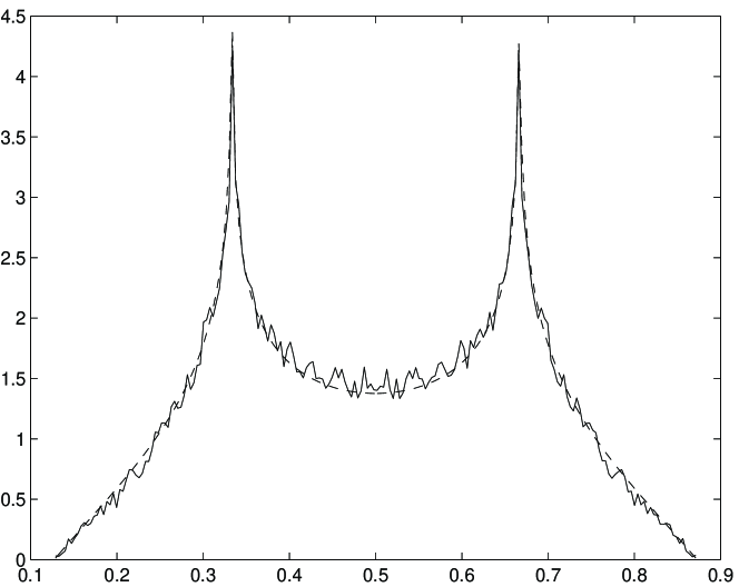
References

  • [1] H. Akaike. On a successive transformation of probability distribution and its application to the analysis of the optimum gradient method. Ann. Inst. Statist. Math. Tokyo, 11:1–16, 1959.
  • [2] J. Barzilai and J.M. Borwein. Two-point step size gradient methods. IMA Journal of Numerical Analysis, 8:141–148, 1988.
  • [3] E.G. Birgin and J.M. Martínez. A spectral conjugate gradient method for unconstrained optimization. Applied Mathematics and Optimization, 43:117–128, 2001.
  • [4] V.V. Fedorov. Theory of Optimal Experiments. Academic Press, New York, 1972.
  • [5] G.E. Forsythe. On the asymptotic directions of the s𝑠s-dimensional optimum gradient method. Numerische Mathematik, 11:57–76, 1968.
  • [6] J. Hale and H. Koçak. Dynamics and Bifurcations. Springer-Verlag, Heidelberg, 1991.
  • [7] L.V. Kantorovich and G.P. Akilov. Functional Analysis. Pergamon Press, London, 1982. Second edition.
  • [8] J. Kiefer and J. Wolfowitz. The equivalence of two extremum problems. Canadian Journal of Mathematics, 12:363–366, 1960.
  • [9] V.S. Kozjakin and M.A. Krasnosel’skii. Some remarks on the method of minimal residues. Numer. Funct. Anal. and Optimiz., 4(3):211–239, 1982.
  • [10] M.A. Krasnosel’skii and S.G. Krein. An iteration process with minimal residues. Mat. Sb. (in Russian), 31(4):315–334, 1952.
  • [11] J.P. LaSalle. The Stability of Dynamical Systems. SIAM, Philadelphia, 1976.
  • [12] D.G. Luenberger. Introduction to Linear and Nonlinear Programming. Addison-Wesley, Reading, Massachusetts, 1973.
  • [13] J. Nocedal, A. Sartenaer, and C. Zhu. On the accuracy of nonlinear optimization algorithms. Technical Report Nov. 1998, ECE Department, Northwestern Univ., Evanston, Il 60208, 1998.
  • [14] J. Nocedal, A. Sartenaer, and C. Zhu. On the behavior of the gradient norm in the steepest descent method. Computational Optimization and Applications, 22:5–35, 2002.
  • [15] L. Pronzato, H.P. Wynn, and A.A. Zhigljavsky. Dynamical Search. Chapman & Hall/CRC, Boca Raton, 2000.
  • [16] L. Pronzato, H.P. Wynn, and A.A. Zhigljavsky. Renormalised steepest descent in Hilbert space converges to a two-point attractor. Acta Applicandae Mathematicae, 67:1–18, 2001.
  • [17] L. Pronzato, H.P. Wynn, and A.A. Zhigljavsky. Kantorovich-type inequalities for operators via D-optimal design theory. Linear Algebra and Its Applications (Special Issue on Linear Algebra and Statistics), 2005. to appear.
  • [18] M. Raydan. The Barzilai and Borwein gradient method for the large scale unconstrained minimization problem. SIAM Journal Optimization, 7(1):26–33, 1997.
  • [19] M. Raydan and B.F. Svaiter. Relaxed steepest descent and Cauchy-Barzilai-Borwein method. Computational Optimization and Applications, 21:155–167, 2002.
  • [20] A.N. Shiryaev. Probability. Springer, Berlin, 1996.
  • [21] S.D. Silvey. Optimal Design. Chapman & Hall, London, 1980.