Two phase partially miscible flow and transport modeling in porous media ; application to gas migration in a nuclear waste repository

Abstract

We derive a compositional compressible two-phase, liquid and gas, flow model for numerical simulations of hydrogen migration in deep geological repository for radioactive waste. This model includes capillary effects and the gas high diffusivity. Moreover, it is written in variables (total hydrogen mass density and liquid pressure) chosen in order to be consistent with gas appearance or disappearance. We discuss the well possedness of this model and give some computational evidences of its adequacy to simulate gas generation in a water saturated repository.

1 Introduction

The simultaneous flow of immiscible fluids in porous media occurs in a wide variety of applications. The most concentrated research in the field of multiphase flows over the past four decades has focused on unsaturated groundwater flows, and flows in underground petroleum reservoirs. Most recently, multiphase flows have generated serious interest among engineers concerned with deep geological repository for radioactive waste. There is growing awareness that the effect of hydrogen gas generation, due to anaerobic corrosion of the steel engineered barriers (carbon steel overpack and stainless steel envelope) of radioactive waste packages, can affect all the functions allocated to the canisters, waste forms, buffers, backfill, host rock. Host rock safety function may be threaten by overpressurisation leading to opening fractures of the host rock, inducing groundwater flow and transport of radionuclides.

The equations governing these flows are inherently nonlinear, and the geometries and material properties characterizing many problems in many applications can be quite irregular and contrasted. As a result, numerical simulation often offers the only viable approach to the mathematical modeling of multiphase flows. In nuclear waste management, the migration of gas through the near field environment and the host rock, involves two components, water and pure hydrogen $\text{H}_{2}$; and two phases ”liquid” and ”gas”. It is then not clear if conventional models, like for instance the Black-Oil model, used in petroleum or groundwater engineering are still valid for such a situation. Our ability to understand and predict underground gas migration is crucial to the design of reliable waste storages. This is a fairly new frontier in multiphase porous-media flows, and again the inherent complexity of the physics leads to governing equations for which the only practical way to produce solutions may be numerical simulation. This exposition provides an overview of the types of standard models that are used in the field of compressible multiphase multispecies flows in porous media and includes discussions of the problems coming from $\text{H}_{2}$  gas being one of the components. Finally the paper also addresses one of the outstanding physical and mathematical problems in multiphase flow simulation: the appearance disappearance of one of the phases, leading to the degeneracy of the equations satisfied by the saturation. It has been seen recently in a benchmark organized by the French agency in charge of the Nuclear Waste management in France Bench that none of the usual codes used in that field where able to simulate adequately the appearance or/and disappearance of one of the phases. In order to overcome this difficulty, we will discuss a formulation based on new variables which doesn’t degenerate. We will demonstrate through two test cases, the ability of this new formulation to actually cope with the appearance or/and disappearance of one phase. The scope of the paper is limited to isothermal flows in rigid porous media and will not include the possible process of ”pathway dilation” as described in Hors .

2 Conceptual and mathematical model

Our goal is first to present a survey of the conventional models used for describing two-phase two-components flow in porous media. Most of these models have been designed and widely used in petroleum engineering (see for instance: Allen , Bear:1 , ChJa , DPeace , ECLIPSE ). We consider herein a porous medium saturated with a fluid composed of 2 phases : liquid and gas. According to the application we have in mind, the fluid is a mixture of two components: water (mostly liquid) and hydrogen ($\text{H}_{2}$, mostly gas). Water is present in the gas phase through vaporization, and hydrogen is present in the liquid phase through dissolution. The fluids are compressible and the model is assumed to be isothermal. For simplicity, we assume first the porous medium to be rigid, meaning the porosity $\Phi$ is only a function of the space variable $\Phi=\Phi(\mbox{\bf x})$; and second, we neglect the pressure induced dilation of gas pathways. Hydrogen being highly diffusive we have described in detail how the diffusion could be taken in account in the models.

2.1 Petrographic and fluid properties

2.1.1 Fluid phases

The two phases will be denoted by indices $l$, for liquid and $g$ for gas. Associated to each phase in the porous media are the following quantities:

• liquid and gas phase pressures: $p_{l}$, $p_{g}$;

• liquid and gas phase saturations: $S_{l}$, $S_{g}$;

• liquid and gas phase mass densities: $\rho_{l}$, $\rho_{g}$;

• liquid and gas phase viscosities: $\mu_{l}$, $\mu_{g}$;

• phase volumetric flow rates, $\mathbf{q}_{l}$ and $\mathbf{q}_{g}$;

Then, the Darcy-Muskat law says:

$$\mbox{$\mathbf{q}_{l}$}=-\mathbb{K}(\mbox{\bf x})\frac{kr_{l}(S_{l})}{\mu_{l}}\left(\mbox{$\nabla$}p_{l}-\rho_{l}\mbox{$\mathbf{g}$}\right),\quad\mbox{$\mathbf{q}_{g}$}=-\mathbb{K}(\mbox{\bf x})\frac{kr_{g}(S_{g})}{\mu_{g}}\left(\mbox{$\nabla$}p_{g}-\rho_{g}\mbox{$\mathbf{g}$}\right),$$ (1)

where $\mathbb{K}(\mbox{\bf x})$ is the absolute permeability tensor, $kr_{l}$ and $kr_{g}$ are the relative permeability functions, and $\mathbf{g}$ is the gravity acceleration.

The above phase mass densities and viscosities are all functions of phase pressures and of phase composition. Moreover, phase saturations satisfy

$$S_{l}+S_{g}=1$$ (2)

and the pressures are connected through a given experimental capillary pressure law:

$$p_{c}(S_{g})=p_{g}-p_{l}.$$ (3)

From definition (3) we should notice that $p_{c}$ is strictly increasing function of gas saturation, $p_{c}^{\prime}(S_{g})>0$.

2.1.2 Fluid components

Water and pure hydrogen components will be denoted by indices $w$ and $h$. Since the liquid phase could be composed of water and dissolved hydrogen we need to introduce the water mass density in the liquid phase $\rho_{l}^{w}$, and the hydrogen mass density in the liquid phase $\rho_{l}^{h}$. Similarly, we introduce the water and hydrogen mass densities in the gas phase: $\rho_{g}^{w}$, $\rho_{g}^{h}$. Note that the upper index is always the component index, and the lower one denotes the phase. We have, then

$$\rho_{l}=\rho_{l}^{w}+\rho_{l}^{h},\quad\rho_{g}=\rho_{g}^{w}+\rho_{g}^{h}.$$ (4)

Since the composition of each phase is generally unknown we introduce the mass fraction of the component $i\in\{w,h\}$ in the phase $\alpha\in\{g,l\}$

$$\omega_{\alpha}^{i}=\frac{\rho_{\alpha}^{i}}{\rho_{\alpha}};\quad\omega_{\alpha}^{w}+\omega_{\alpha}^{h}=1,\;\alpha\in\{g,l\}.$$ (5)

2.2 Mass conservation equation

The conservation of the mass applies to each component $i$ and reads, for any arbitrary control volume ${\cal R}$:

$$\frac{dm^{i}}{dt}+F^{i}={\cal F}^{i}\;,\;\;i\in\{w,h\}.$$ (6)

where

• $m^{i}$ is the mass of the component $i$, in the control volume ${\cal R}$, at given instant $t$;

• $F^{i}$ is the rate at which the component $i$ is leaving (migrating from) the volume ${\cal R}$, at given instant $t$;

• ${\cal F}^{i}$ is the source term (the rate at which the $i$ component is added to ${\cal R}$ by the source).

The mass of each component $i$ is a sum over all phases $g$ and $l$:

$$m^{i}=\int_{\cal R}\Phi\left(S_{l}\rho_{l}\omega_{l}^{i}+S_{g}\rho_{g}\omega_{g}^{i}\right)\,d\mbox{\bf x},\quad i\in\{w,h\}.$$

In each phase, the migration of a component is due to the transport by the phase velocity and to the molecular diffusion:

$$F^{i} =\int_{\partial{\cal R}}\left(\rho_{l}\omega_{l}^{i}\mbox{$\mathbf{q}_{l}$}+\rho_{g}\omega_{g}^{i}\mbox{$\mathbf{q}_{g}$}+\mbox{$\mathbf{j}_{l}^{i}$}+\mbox{$\mathbf{j}_{g}^{i}$}\right)\cdot{\bf n}\,d\mbox{\bf x};\;\;i\in\{w,h\};$$

where ${\bf n}$ is the unit outer normal to ${\partial{\cal R}}$. The phase flow velocities, $\mathbf{q}_{l}$ and $\mathbf{q}_{g}$ are given by the Darcy-Muskat law (1), and the component $i$ diffusive flux in phase $\alpha$ is denoted $\mathbf{j}_{\alpha}^{i}$, $i\in\{w,h\}$, $\alpha\in\{g,l\}$, and will be defined in the next paragraph, by equations (12). From (6) we get the differential equations:

$$\Phi\frac{\partial}{\partial t}\left(S_{l}\rho_{l}\omega_{l}^{w}+S_{g}\rho_{g}\omega_{g}^{w}\right)+\mbox{$\mbox{div}$}\left(\rho_{l}\omega_{l}^{w}\mbox{$\mathbf{q}_{l}$}+\rho_{g}\omega_{g}^{w}\mbox{$\mathbf{q}_{g}$}+\mbox{$\mathbf{j}_{l}^{w}$}+\mbox{$\mathbf{j}_{g}^{w}$}\right)={\cal F}^{w},$$ (7)

$$\Phi\frac{\partial}{\partial t}\left(S_{l}\rho_{l}\omega_{l}^{h}+S_{g}\rho_{g}\omega_{g}^{h}\right)+\mbox{$\mbox{div}$}\left(\rho_{l}\omega_{l}^{h}\mbox{$\mathbf{q}_{l}$}+\rho_{g}\omega_{g}^{h}\mbox{$\mathbf{q}_{g}$}+\mbox{$\mathbf{j}_{l}^{h}$}+\mbox{$\mathbf{j}_{g}^{h}$}\right)={\cal F}^{h}.$$ (8)

2.2.1 Diffusion fluxes

From $M^{w}$ and $M^{h}$, the water and hydrogen molar masses, using definitions (5) we define the following water and hydrogen molar concentrations in each phase $\alpha\in\{g,l\}$:

$$c_{\alpha}^{h}=\frac{S_{\alpha}\rho_{\alpha}^{h}}{M^{h}}=\frac{S_{\alpha}\rho_{\alpha}\omega_{\alpha}^{h}}{M^{h}},\quad c_{\alpha}^{w}=\frac{S_{\alpha}\rho_{\alpha}^{w}}{M^{w}}=\frac{S_{\alpha}\rho_{\alpha}\omega_{\alpha}^{w}}{M^{w}}.$$ (9)

Then the phase $\alpha$ molar concentrations, $\alpha\in\{g,l\}$, is:

$$c_{\alpha}=c_{\alpha}^{h}+c_{\alpha}^{w}=S_{\alpha}\rho_{\alpha}\left(\frac{\omega_{\alpha}^{h}}{M^{h}}+\frac{\omega_{\alpha}^{w}}{M^{w}}\right).$$ (10)

Usually, component $i$ diffusive flux in phase $\alpha$ is assumed to be depending on $X_{\alpha}^{i}$, the component $i$ molar fraction in phase $\alpha\in\{g,l\}$, defined from (9) and (10):

$$X_{\alpha}^{h}=\frac{c_{\alpha}^{h}}{c_{\alpha}}=\frac{\omega_{\alpha}^{h}}{\omega_{\alpha}^{h}+(M^{h}/M^{w})\omega_{\alpha}^{w}},\quad X_{\alpha}^{w}=\frac{c_{\alpha}^{w}}{c_{\alpha}}=\frac{\omega_{\alpha}^{w}}{\omega_{\alpha}^{w}+(M^{w}/M^{h})\omega_{\alpha}^{h}};\quad\sum_{i=h,w}X_{\alpha}^{i}=1,$$ (11)

for $\alpha\in\{l,g\}$. Molar diffusive flux of component $i$ in phase $\alpha\in\{g,l\}$ is given by

$$\mathbf{J}_{\alpha}^{i}=-c_{\alpha}D_{\alpha}^{i}\mbox{$\nabla$}X_{\alpha}^{i};\quad\alpha\in\{g,l\},\quad i\in\{w,h\}$$

and give molar diffusive flow rate of component $i$ through the unit area. Coefficients $D_{\alpha}^{h}$ and $D_{\alpha}^{w}$ (unit $L^{2}/T$) are Darcy scale molecular diffusion coefficients of components in phase $\alpha\in\{g,l\}$. Mass flux of component $i$ in phase $\alpha$, in equations (7), (8) is then obtained by multiplying the above component molar diffusive fluxes, $\mathbf{J}_{\alpha}^{i}$, by the molar mass $M_{i}$ of the component $i$, and by the rock porosity:

$$\mathbf{j}_{\alpha}^{h}=-\Phi M^{h}c_{\alpha}D_{\alpha}^{h}\mbox{$\nabla$}X_{\alpha}^{h},\quad\mathbf{j}_{\alpha}^{w}=-\Phi M^{w}c_{\alpha}D_{\alpha}^{w}\mbox{$\nabla$}X_{\alpha}^{w}.$$ (12)

Remark 1

: Number of unknowns in the system is eight: $S_{l},\rho_{l}^{w},\rho_{l}^{h},p_{l},S_{g},\rho_{g}^{w},\rho_{g}^{h},p_{g}$; but, up to now, we have only four equations (2), (3), (7) and (8), and therefore, four additional equations are needed to close the system.

Remark 2

: Note that $D_{\alpha}^{h}$ and $D_{\alpha}^{w}$ are not exactly molecular diffusion coefficients in phase $\alpha$, corresponding to molecule-molecule interactions in free space but $\Phi D_{\alpha}^{i}$, $\alpha\in\{g,l\}$, $i\in\{w,h\}$, are effective diffusion coefficients, obtained from the strict molecular diffusion coefficients by a kind of averaging through the whole porous medium (see section 2.6 in Bear:1 , or Milli or Jin ). Moreover, for simplicity, we have not included in diffusion of component $i$ in phase $\alpha$ any dependancy on phase saturations; and then did not consider possible non linear effects coming from coupling between advective-diffusive transport (”dusty gas” model) and molecular streaming effects (Knutsen diffusion) (see for instance Tough ).

Remark 3

In a binary system diffusive fluxes satisfy $\mathbf{j}_{\alpha}^{h}+\mathbf{j}_{\alpha}^{w}=0$, for $\alpha\in\{g,l\}$, and therefore we have

$$M^{h}D^{h}_{\alpha}=M^{w}D^{w}_{\alpha},\quad\alpha\in\{g,l\}.$$ (13)

2.3 Phase equilibrium Black-oil model

The additional equations needed to close the system of equations (2), (3), (7) and (8) will come from the assumption that the two phases are in equilibrium; equilibrium meaning that at any time the quantity of hydrogen dissolved in the water is maximal for the given pressure, and similarly, the quantity of evaporated water is maximal for the given pressure. Composition of each phase is then uniquely determined by its phase pressure and saturation. In this flow situation we say that water and gas phases are saturated. Nevertheless it could happen that one of the phases disappears: either water can completely evaporate or hydrogen can be completely dissolved in the water. Then in these situations the composition of the remaining phase is not uniquely determined by its phase pressure, and the phase composition becomes an independent variable (instead of the saturation which is now constant, 0 or 1). This flow situation correspond to the so-called unsaturated flow. For unsaturated flow, standard practice in petroleum reservoir engineering is to introduce the following quantities:

• liquid and gas formation volume factors, $B_{l}=B_{l}(p_{l})$, $B_{g}=B_{g}(p_{g})$;

• solution gas/liquid phase Ratio $R_{s}=R_{s}(p_{l})$;

• vapor water/gas phase Ratio $R_{v}=R_{v}(p_{g})$.

The explanation of formation volume factors and solution component/phase ratios, as used in the oil reservoir modelling, is as follows. Considering the volume $\Delta V_{l}^{res}$ of liquid at reservoir conditions (reservoir temperature and pressure); when this volume of liquid is transported through the tubing to the surface it separates at standard conditions to a volume of liquid $\Delta V_{l}^{std}$, and a volume of gas $\Delta V_{g}^{std}$ (coming out of the liquid, due to the pressure drop). At standard (i.e. stock tank) conditions, the liquid phase contains only oil component (here only water component) and the gas phase contains only gas component (here only hydrogen). Then applying conservation of mass,

$$\Delta V_{l}^{res}\rho_{l}=\Delta V_{l}^{std}\rho_{l}^{std}+\Delta V_{g}^{std}\rho_{g}^{std};$$

and denoting the solution gas/liquid Ratio $R_{s}={\Delta V_{g}^{std}}/{\Delta V_{l}^{std}}$, we may write:

$$\Delta V_{l}^{res}\rho_{l}=\Delta V_{l}^{std}(\rho_{l}^{std}+R_{s}\rho_{g}^{std}),$$

and the liquid phase mass density decomposition

$$\rho_{l}=\frac{\rho_{l}^{std}+R_{s}\rho_{g}^{std}}{B_{l}},$$ (14)

where $B_{l}$ is the liquid formation volume factor, $B_{l}={\Delta V_{l}^{res}}/{\Delta V_{l}^{std}}$. Similarly, from $\Delta V_{g}^{res}\rho_{g}$ and the gas formation volume factor $B_{g}={\Delta V_{g}^{res}}/{\Delta V_{g}^{std}}$, we get the gas phase mass density decomposition

$$\rho_{g}=\frac{\rho_{g}^{std}+R_{v}\rho_{l}^{std}}{B_{g}};$$ (15)

where the vapor water/gas phase ratio $R_{v}={\Delta V_{l}^{std}}/{\Delta V_{g}^{std}}$. Now, in order to express the diffusion fluxes in terms of the new variables $R_{s},R_{v},B_{l}$ and $B_{g}$ we have to rewrite the molar concentrations defined in (9):

$$c_{l}^{h}=\frac{S_{l}R_{s}\rho_{g}^{std}}{M^{h}B_{l}},\quad c_{l}^{w}=\frac{S_{l}\rho_{l}^{std}}{M^{w}B_{l}},\quad c_{g}^{h}=\frac{S_{g}\rho_{g}^{std}}{M^{h}B_{g}},\quad c_{g}^{w}=\frac{S_{g}R_{v}\rho_{l}^{std}}{M^{w}B_{g}}.$$ (16)

These concentrations, defined in (16) may be slightly different from those previously defined in (9) if the gas at standard conditions is not composed only of hydrogen, and the liquid, also at standard conditions, is note made only of water. The phase molar concentrations, from (16), are then given by:

$$c_{l}=c_{l}^{h}+c_{l}^{w}=\frac{S_{l}}{B_{l}}\left(\frac{R_{s}\rho_{g}^{std}}{M^{h}}+\frac{\rho_{l}^{std}}{M^{w}}\right)=\frac{S_{l}}{B_{l}}\frac{\rho_{g}^{std}}{M^{h}}(R_{s}+F),$$

$$c_{g}=c_{g}^{h}+c_{g}^{w}=\frac{S_{g}}{B_{g}}\left(\frac{\rho_{g}^{std}}{M^{h}}+\frac{R_{v}\rho_{l}^{std}}{M^{w}}\right)=\frac{S_{g}}{B_{g}}\frac{\rho_{g}^{std}}{M^{h}}(1+FR_{v}),$$

where $F$ is given by:

$$F=\frac{M^{h}\rho_{l}^{std}}{M^{w}\rho_{g}^{std}}.$$ (17)

The component molar fractions in phase, are now defined as:

$$X_{l}^{h} =\frac{c_{l}^{h}}{c_{l}}=\frac{R_{s}\rho_{g}^{std}}{R_{s}\rho_{g}^{std}+(M^{h}/M^{w})\rho_{l}^{std}}=\frac{R_{s}}{R_{s}+F},$$ (18)

$$X_{l}^{w} =\frac{c_{l}^{w}}{c_{l}}=\frac{\rho_{l}^{std}}{\rho_{l}^{std}+(M^{w}/M^{h})R_{s}\rho_{g}^{std}}=\frac{F}{R_{s}+F},$$

$$X_{g}^{h} =\frac{c_{g}^{h}}{c_{g}}=\frac{\rho_{g}^{std}}{\rho_{g}^{std}+(M^{h}/M^{w})R_{v}\rho_{l}^{std}}=\frac{1}{1+FR_{v}},$$

$$X_{g}^{w} =\frac{c_{g}^{w}}{c_{g}}=\frac{R_{v}\rho_{l}^{std}}{R_{v}\rho_{l}^{std}+(M^{w}/M^{h})\rho_{g}^{std}}=\frac{FR_{v}}{1+FR_{v}}.$$

Mass diffusive fluxes of components, defined in (12), depend on component molar fractions in phases; they have then to be rewritten. For instance, the mass diffusion flux of hydrogen in water, takes now the form:

$$\mbox{$\mathbf{j}_{l}^{h}$}/\rho_{g}^{std} =-\Phi\frac{M^{h}}{\rho_{g}^{std}}\frac{S_{l}}{B_{l}}\frac{\rho_{g}^{std}}{M^{h}}\left(R_{s}+F\right)D_{l}^{h}\mbox{$\nabla$}X_{l}^{h}=-\Phi\frac{S_{l}}{B_{l}}\frac{F}{R_{s}+F}D_{l}^{h}\mbox{$\nabla$}R_{s}.$$

Other diffusion fluxes could be obtained by similar calculations, leading to the following formulas:

$$\boldsymbol{\phi}_{l}^{h}=\mbox{$\mathbf{j}_{l}^{h}$}/\rho_{g}^{std} =-\Phi\frac{S_{l}}{B_{l}}\frac{F}{R_{s}+F}D_{l}^{h}\mbox{$\nabla$}R_{s},\quad\boldsymbol{\phi}_{l}^{w}=\mbox{$\mathbf{j}_{l}^{w}$}/\rho_{l}^{std}=\Phi\frac{S_{l}}{B_{l}}\frac{1}{R_{s}+F}D_{l}^{w}\mbox{$\nabla$}R_{s},$$ (19)

$$\boldsymbol{\phi}_{g}^{h}=\mbox{$\mathbf{j}_{g}^{h}$}/\rho_{g}^{std} =\Phi\frac{S_{g}}{B_{g}}\frac{F}{1+FR_{v}}D_{g}^{h}\mbox{$\nabla$}R_{v},\quad\boldsymbol{\phi}_{g}^{w}=\mbox{$\mathbf{j}_{g}^{w}$}/\rho_{l}^{std}=-\Phi\frac{S_{g}}{B_{g}}\frac{1}{1+FR_{v}}D_{g}^{w}\mbox{$\nabla$}R_{v}.$$ (20)

Remark 4

Let us recall, like in Remark 13, that the diffusion coefficients satisfy $M^{h}D_{l}^{h}=M^{w}D_{l}^{w}$, $M^{h}D_{g}^{h}=M^{w}D_{g}^{w}$; and, like in (11), $\sum_{i=h,w}X^{i}_{\alpha}=1,$ for any phase $\alpha\in\{l,g\}$, in (18).

The Darcy fluxes (1) can now be rewritten in the following form:

$$\mbox{$\mathbf{q}_{l}$}=-\mathbb{K}\frac{kr_{l}}{\mu_{l}}\left(\mbox{$\nabla$}p_{l}-\frac{\rho_{l}^{std}+R_{s}\rho_{g}^{std}}{B_{l}}\mbox{$\mathbf{g}$}\right),\quad\mbox{$\mathbf{q}_{g}$}=-\mathbb{K}\frac{kr_{g}}{\mu_{g}}\left(\mbox{$\nabla$}p_{g}-\frac{\rho_{g}^{std}+R_{v}\rho_{l}^{std}}{B_{g}}\mbox{$\mathbf{g}$}\right),$$

and the component fluxes, normalized by standard densities, are,

$$\boldsymbol{\phi}^{w}=\frac{1}{B_{l}}\mbox{$\mathbf{q}_{l}$}+\frac{R_{v}}{B_{g}}\mbox{$\mathbf{q}_{g}$}+\boldsymbol{\phi}_{l}^{w}+\boldsymbol{\phi}_{g}^{w},\quad\boldsymbol{\phi}^{h}=\frac{R_{s}}{B_{l}}\mbox{$\mathbf{q}_{l}$}+\frac{1}{B_{g}}\mbox{$\mathbf{q}_{g}$}+\boldsymbol{\phi}_{l}^{h}+\boldsymbol{\phi}_{g}^{h}.$$ (21)

Finally, we can write mass conservation (7), (8) in the following form:

$$\Phi\frac{\partial}{\partial t}\left(\frac{S_{l}}{B_{l}}+\frac{R_{v}S_{g}}{B_{g}}\right)+\mbox{$\mbox{div}$} \left(\boldsymbol{\phi}^{w}\right)={\cal F}^{w}/\rho_{l}^{std},$$ (22)

$$\Phi\frac{\partial}{\partial t}\left(\frac{S_{l}R_{s}}{B_{l}}+\frac{S_{g}}{B_{g}}\right)+\mbox{$\mbox{div}$} \left(\boldsymbol{\phi}^{h}\right)={\cal F}^{h}/\rho_{g}^{std}.$$ (23)

These equations have to be completed by equations (2) and (3). For instance, in (22) and (23), we can take saturation and one of the pressures as independent variables; for example $S_{g}$ and $p_{l}$, and for the other terms the following functional dependencies:

$$B_{l}(p_{l}),B_{g}(p_{g}),R_{s}(p_{l}),R_{v}(p_{g}),\mu_{l}(p_{l}),\mu_{g}(p_{g}),kr_{w}(S_{g}),kr_{g}(S_{g}).$$

According to their definition, $F$, $\rho_{g}^{std}$, $\rho_{l}^{std}$ and $D^{i}_{\alpha}$ ($\alpha\in\{l,g\},i\in\{w,h\}$) are constants, and $\Phi$ and $\mathbb{K}$ are depending only on space position.

2.3.1 Unsaturated flow

Equations (22) and (23), with saturation and pressure as unknowns, are valid if there is no missing phase (saturated flow); but if one of the phases is missing (unsaturated flow), equations and unknowns have to be adapted. There are two possible unsaturated cases, according to either the gas phase or the liquid phase disappears :

1. Gas phase missing (Hydrogen totally dissolved in water): then we have $S_{g}=0$, $S_{l}=1$. Generalized gas phase Darcy’s velocity is equal to zero since $kr_{g}(0)=0$. Independent variables are now $p_{l}$, the liquid phase pressure, and $R_{s}$, the solution gas/liquid phase Ratio; then we must write $B_{l}=B_{l}(p_{l},R_{s})$ and $\mu_{l}=\mu_{l}(p_{l},R_{s})$, for $0\leq R_{s}\leq\hat{R}_{s}(p_{l})$, where $\hat{R}_{s}(p_{l})$ is equilibrium solution gas/liquid phase ratio.

2. Liquid phase missing: then, $S_{l}=0$, $S_{g}=1$. Generalized liquid phase Darcy’s velocity is zero since $kr_{w}(S_{g}=1)=0$; independent variables are now $p_{g}$, the gas phase pressure, and $R_{v}$ the water vapor/gas phase ratio, become the new independent variables. However pressure $p_{l}$ can be kept as independent variable since $p_{g}$ could be expressed through the capillary pressure law (3). We must also write $B_{g}=B_{g}(p_{g},R_{v})$ and $\mu_{g}=\mu_{g}(p_{g},R_{v})$, for $0\leq R_{v}\leq\hat{R}_{v}(p_{g})$, where $\hat{R}_{v}(p_{g})$ is the equilibrium water vapor/gas phase ratio.

These above conditions can be summarized as

$$S_{g}\geq 0,\quad\hat{R}_{s}(p_{l})-R_{s}\geq 0,\quad(\hat{R}_{s}(p_{l})-R_{s})S_{g}=0,$$ (24)

$$S_{l}\geq 0,\quad\hat{R}_{v}(p_{g})-R_{v}\geq 0,\quad(\hat{R}_{v}(p_{g})-R_{v})S_{l}=0.$$ (25)

Remark 5

In this last section, Phase Equilibrium Black-oil model, we did not take in account a possible interplay between dissolution and capillary pressure. $\;\Box$

2.4 Thermodynamical equilibrium Henry-Raoult model

Another way of closing the system of equations (2), (3), (7) and (8) is to use phase thermodynamical properties for characterizing equilibrium . We use first ideal gas law and Dalton law,

$$p_{g}=p_{g}^{w}+p_{g}^{h},$$ (26)

where $p_{g}^{w}$ and $p_{g}^{h}$ are the vaporized water and hydrogen partial pressures in the gas phase; and

$$p_{g}^{w}=\frac{\rho_{g}^{w}}{M^{w}}RT,\quad p_{g}^{h}=\frac{\rho_{g}^{h}}{M^{h}}RT.$$ (27)

$T$ is the temperature, $R$ is universal gas constant and $M^{w}$, $M^{h}$ are the water and hydrogen molar masses.

Next, we apply Henry’s and Raoult’s laws which say that, at equilibrium, the vapor pressure of a substance varies linearly with its mole fraction in solution. In Henry’s law the constant of proportionality is obtained by experiment and in Raoult’s law the constant is the pressure of the component in its pure state. Here we will assume, for simplicity, that the quantity of dissolved hydrogen in the liquid is small; then these laws reduce to the linear Henry’s law, which says that the amount of gas dissolved in a given volume of the liquid phase is directly proportional to the partial pressure of that same gas in the gas phase:

$$\rho_{l}^{h}=H(T)M^{h}p_{g}^{h},$$ (28)

where $H(T)$ is the Henry’s law constant, depending only on the temperature. For the liquid phase, we apply Raoult’s law which says that the water vapor pressure is equal to the vapor pressure of the pure solvent, at given temperature, multiplied by the mole fraction of the solvent. The water vapor partial pressure of the pure solvent depends only on the temperature and therefore is a constant, denoted here by $\hat{p}_{g}^{w}(T)$, so we have from definition (9)

$$p_{g}^{w}=\hat{p}_{g}^{w}(T)X_{l}^{w}=\hat{p}_{g}^{w}(T)\frac{\rho_{l}^{w}}{\rho_{l}^{w}+(M^{w}/M^{h})\rho_{l}^{h}}.$$ (29)

Further on, we can include in formula (29) the presence of capillary pressure, by using Kelvin’s equation (see Abbas ) which gives:

$$p_{g}^{w}=\hat{p}_{g}^{w}(T)\frac{\rho_{l}^{w}}{\rho_{l}^{w}+(M^{w}/M^{h})\rho_{l}^{h}}e^{-M^{w}p_{c}/(RT\rho_{l})}.$$ (30)

If now, to equations (26)-(28) and (30) we add the relations

$$\rho_{l}^{h}+\rho_{l}^{w}=\rho_{l},\quad\rho_{g}^{h}+\rho_{g}^{w}=\rho_{g},$$ (31)

and the water compressibility, defined by

$$\rho_{l}^{w}=\frac{\rho_{l}^{std}}{B_{l}(p_{l})};$$ (32)

then, we have 8 equations: (26), (27)_1,2, (28), (30), (31)_1,2 and (32) and 10 unknowns:

$$p_{l},p_{g},p_{g}^{w},p_{g}^{h},\rho_{l}^{h},\rho_{l}^{w},\rho_{l},\rho_{g}^{h},\rho_{g}^{w},\rho_{g}.$$

We may, for instance, parametrize all these 10 unknowns, by the two phase pressures $p_{l}$ and $p_{g}$. For this we should combine the Henry law (28), the Raoult-Kelvin law (30) and (26) leading to the system of two equations for $p_{g}^{h}$ and $p_{g}^{w}$:

$$p_{g}^{w} =\hat{p}_{g}^{w}(T)\frac{\rho_{l}^{w}}{\rho_{l}^{w}+(M^{w}H(T))p_{g}^{h}}e^{-M^{w}(p_{g}-p_{l})/(RT(\rho_{l}^{w}+M^{h}H(T)p_{g}^{h})}$$

$$p_{g} =p_{g}^{w}+p_{g}^{h}.$$

It is easy to show that this above system of two equations has a unique solution $p_{g}^{w},p_{g}^{h}>0$ for any $p_{g}\geq\hat{p}_{g}^{w}(T)$; and solving this system we obtain

$$p_{g}^{w}=f(p_{g},p_{l}),\quad p_{g}^{h}=g(p_{g},p_{l}).$$

By (27)_1,2 we can then write $\rho_{g}^{h}$, $\rho_{g}^{w}$ and $\rho_{g}$ as functions of $p_{l}$ and $p_{g}$, and by (28) and (32) we can finally express $\rho_{l}^{h}$, $\rho_{l}^{w}$ and $\rho_{l}$ as functions of the phase pressures.

Remark 6

The gas phase will appear only if there is a sufficient quantity of dissolved hydrogen in the liquid phase, and this quantity is exactly the dissolved gas quantity, at equilibrium, given by Henry’s law. But when the dissolved gas (hydrogen) quantity is smaller than the quantity of hydrogen at equilibrium, then the Henry law does not apply; and $S_{g}$ is then equal to zero and could not be taken as unknown. In this situation, instead of saturation, we may take $\rho_{l}^{h}$ as independent variable. We notice that Henry-Raoult model based on thermodynamical equilibrium leads to a similar concepts as the ones developed for establishing Black Oil model for reservoir modeling. $\;\Box$

Remark 7

In the Henry-Raoult model, if there is no vaporized water, $p_{g}=p_{h}^{g}$, the criteria for non saturated flow is simple and reads

$$\frac{\rho_{l}^{h}}{M^{h}H(T)}<p_{g}=p_{l}+p_{c}(0),$$ (33)

if there is a threshold pressure, i.e. $p_{c}(0)\neq 0$. The same criterion can be used also if there is vaporized water, as long as the pressure in porous medium is much larger than vaporized water pressure.

Remark 8

In Henry-Raoult model, above, we were assuming for simplicity, no complete evaporation of the water.

2.4.1 Comparison of Equilibrium models

We will now consider in more details a special case, where we may, from the Henry-Raoult model, get back the Black oil model. In both models we will then use diffusive fluxes developed in Section 2.3. For simplicity, we will neglect in (29) influence of capillary pressure and solved gas on water vapor partial pressure, leading to $p_{g}^{w}=\hat{p}_{g}^{w}(T)$ being a constant. Then we have from (28), (32) and (31)

$$\rho_{l}=\rho_{l}^{h}+\rho_{l}^{w}=H(T)M^{h}p_{g}^{h}+\frac{\rho_{l}^{std}}{B_{l}(p_{l})}=\frac{\rho_{l}^{std}+B_{l}(p_{l})H(T)M^{h}(p_{g}-\hat{p}_{g}^{w}(T))}{B_{l}(p_{l})},$$ (34)

and also from (27),

$$\rho_{g} =\rho_{g}^{h}+\rho_{g}^{w}=\frac{M^{h}}{RT}(p_{g}-\hat{p}_{g}^{w}(T))+\frac{M^{w}}{RT}\hat{p}_{g}^{w}(T).$$ (35)

Therefore, equations (34) and (35) can be written in a form similar to (14)-(15) by defining the gas formation volume factor $B_{g}$, solution gas/liquid phase ratio $R_{s}$ and vapor water/gas phase ratio $R_{v}$, from above thermodynamical relations:

$$\quad R_{s}=B_{l}(p_{l})\frac{H(T)M^{h}}{\rho_{g}^{std}}(p_{g}-\hat{p}_{g}^{w}(T))$$ (36)

$${B_{g}}=\frac{RT\rho_{g}^{std}}{M^{h}(p_{g}-\hat{p}_{g}^{w}(T))},\quad R_{v}=\frac{1}{F}\frac{\hat{p}_{g}^{w}(T)}{p_{g}-\hat{p}_{g}^{w}(T)},$$ (37)

where $F$ is given by (17).

Compared to the Black-Oil model, Section 2.3, here, it is clear from (36) that solution gas/liquid phase ratio $R_{s}$ depends on $p_{l}$ and $p_{g}$ and not only on $p_{l}$.

Remark 9

For the case without any water vapor, the corresponding thermodynamical model is obtained simply by taking $\hat{p}_{g}^{w}(T)=0$ in (36), (37) and $R_{v}=0$ in equations (22) and (23). In the same way, if we neglect dissolved hydrogen, the corresponding thermodynamical model is obtained simply by taking $H(T)=0$ in (36), (37), and $R_{s}=0$ in (22) and (23). $\;\Box$

2.4.2 Model assuming water incompressibility and no water vaporization

In the Henry-Raoult model we assume now that the water is incompressible and the water vapor quantity is neglectful; i.e. the gas phase contains only hydrogen, then (see Remark 33) $p^{h}_{g}\equiv p_{g}$ and $p_{g}^{w}=\hat{p}_{g}^{w}(T)=0$ in (37) leading to $R_{v}\equiv 0$. Formulas (36), (37), could be rewritten as

$$B_{l}\equiv 1, \quad R_{s}=C_{h}p_{g},\quad\frac{1}{B_{g}}=C_{v}p_{g};$$ (38)

where we have denoted

$$C_{h}=\frac{H(T)M^{h}}{\rho_{g}^{std}},\quad C_{v}=\frac{M^{h}}{RT\rho_{g}^{std}};$$ (39)

and equations (14)-(15) become:

$$\rho_{l}(R_{s})=\rho_{l}^{std}+R_{s}\rho_{g}^{std},\quad\rho_{g}(p_{g})=C_{v}\rho_{g}^{std}p_{g}.$$ (40)

Similarly to constant $F$ defined by (17), we use the density ratio

$$G=\frac{\rho_{l}^{std}}{\rho_{g}^{std}},$$ (41)

and equations (22), (23) reduce to

$$\Phi\frac{\partial S_{l}}{\partial t}+\mbox{$\mbox{div}$}\left(\mbox{$\mathbf{q}_{l}$}-\frac{1}{G}\mbox{$\mathbf{J}$}\right)={\cal F}^{w}/\rho_{l}^{std},$$ (42)

$$\Phi\frac{\partial}{\partial t}(S_{l}R_{s}+C_{v}p_{g}S_{g})+\mbox{$\mbox{div}$}\Big{(}R_{s}\mbox{$\mathbf{q}_{l}$}+C_{v}p_{g}\mbox{$\mathbf{q}_{g}$}+\mbox{$\mathbf{J}$}\Big{)}={\cal F}^{h}/\rho_{g}^{std},$$ (43)

$$\mbox{$\mathbf{q}_{l}$}=-\mathbb{K}\frac{kr_{l}}{\mu_{l}}\left(\mbox{$\nabla$}p_{l}-(\rho_{l}^{std}+R_{s}\rho_{g}^{std})\mbox{$\mathbf{g}$}\right),\quad\mbox{$\mathbf{q}_{g}$}=-\mathbb{K}\frac{kr_{g}}{\mu_{g}}\left(\mbox{$\nabla$}p_{g}-C_{v}\rho_{g}^{std}p_{g}\mbox{$\mathbf{g}$}\right),$$ (44)

$$\mbox{$\mathbf{J}$}=-\frac{\Phi S_{l}F}{R_{s}+F}D_{l}^{h}\mbox{$\nabla$}R_{s},$$ (45)

where we have denoted $\boldsymbol{\phi}_{l}^{h}=\mbox{$\mathbf{J}$}$ and used Remark 13 to get $FD_{l}^{h}=GD_{l}^{w}$, from which it follows $\boldsymbol{\phi}_{l}^{w}=-\mbox{$\mathbf{J}$}/G.$

Here there is only hydrogen in phase gas, $p^{h}_{g}=p_{g}$ and Henry’s law assumes thermodynamical equilibrium in which quantity of dissolved hydrogen is proportional to gas phase pressure. In saturated case (where two phases are present) Henry’s law reads $R_{s}=C_{h}p_{g}$, and we can then work with variables $p_{g}$ and $S_{l}$ in equations (42)–(45).

When the gas phase disappears, the gas pressure drops to the liquid pressure augmented by entry pressure, $p_{g}=p_{l}+p_{c}(0)$, the liquid can contain any quantity of dissolved hydrogen $\rho^{h}_{g}$ between zero and $C_{h}\rho_{g}^{std}(p_{l}+p_{c}(0))=H(T)M^{h}(p_{l}+p_{c}(0))$, from Henry’s law (see (28) and definition (39)).

And then, when the gas phase is absent (one of the unsaturated cases) $S_{g}=0$, we will replace saturation, as we did in the Black-Oil model for the same unsaturated case in Section 2.3.1, by a new variable $R_{s}$ (see definitions (28), (36), (39)), such that

$$R_{s}\rho_{g}^{std}=\rho^{h}_{l}$$

is the mass density of dissolved hydrogen in the liquid phase.

Assuming at standard conditions the gas phase contains only hydrogen (hydrogen component mass$\approx$gas phase mass) and the liquid phase contains only water, with water incompressibility and no vaporized water, we see that, in definition (36), $R_{s}=\rho_{l}^{h}/\rho_{g}^{std}\simeq\Delta V_{g}^{std}/\Delta V_{l}^{std}$ which is exactly the definitiion given in the Black-Oil model in Section 2.3.

The physical meaning of $R_{s}$ then stays the same either in Henry-Raoult or in Black-Oil models even in the unsaturated case. Moreover, from mass conservation law it follows that the dissolved hydrogen mass density $R_{s}\rho_{g}^{std}$ is continuous when the gas phase vanishes and this can be expressed as an unilateral condition:

$$0\leq S_{g}\leq 1,\quad 0\leq R_{s}\leq C_{h}p_{g},\quad S_{g}(C_{h}p_{g}-R_{s})=0.$$

In unsaturated region, where $S_{l}=1$ (that is $S_{g}=0$) we replace variable $S_{l}$ by $R_{s}$, and equations (42)–(45) degenerate to:

$$\mbox{$\mbox{div}$}\left(\mbox{$\mathbf{q}_{l}$}-\frac{1}{G}\mbox{$\mathbf{J}$}\right)={\cal F}^{w}/\rho_{l}^{std};$$ (46)

$$\Phi\frac{\partial R_{s}}{\partial t} +\mbox{$\mbox{div}$}\Big{(}R_{s}\mbox{$\mathbf{q}_{l}$}+\mbox{$\mathbf{J}$}\Big{)}={\cal F}^{h}/\rho_{g}^{std};$$ (47)

$$\mathbf{q}_{l} =-\mathbb{K}\lambda_{l}(1)\left(\mbox{$\nabla$}p_{l}-(\rho_{l}^{std}+R_{s}\rho_{g}^{std})\mbox{$\mathbf{g}$}\right);$$ (48)

$$\mathbf{J} =-\frac{\Phi F}{R_{s}+F}D_{l}^{h}\mbox{$\nabla$}R_{s}.$$ (49)

2.5 Saturated/unsaturated state, general formulation

Finally in the saturated region we used $p_{l}$ and $S_{g}$ as variables in (42)–(45) but in unsaturated region we should use other variables, $p_{l}$ and $R_{s}$, in (46)–(49). In order to avoid the change of variables and equations in different regions as above we prefer to introduce a new variable

$$X=(1-S_{g})R_{s}+C_{v}p_{g}S_{g};$$ (50)

in view to make equation (43) parabolic in $X$.

This new variable $X$ is well defined both in saturated and unsaturated regions. Moreover, from (38) and (28), $R_{s}={\rho_{l}^{h}}/{\rho_{g}^{std}}$; from (40) $C_{v}p_{g}={\rho_{g}}/{\rho_{g}^{std}}$ and since $\rho_{g}=\rho_{g}^{h}$, this new variable $X$ is a ”normalized total hydrogen mass density”: $X=(S_{l}\rho_{l}^{h}+S_{g}\rho_{g}^{h})/{\rho_{g}^{std}}$. It is easy then to see that parabolicity is possible only if we take liquid pressure $p_{l}$ as other independent variable. Knowing that in saturated case, $S_{g}>0$, $R_{s}=C_{h}p_{g}$ from Henry’s law, we may write $X$ defined in (50) as:

$$X=\begin{cases}(C_{h}(1-S_{g})+C_{v}S_{g})(p_{l}+p_{c}(S_{g}))&\text{if }S_{g}>0\\ R_{s}&\text{if }S_{g}=0.\end{cases}$$ (51)

Since for capillary pressure defined as a function of gas saturation we have $p_{c}^{\prime}(S_{g})>0$, and since usually, like for hydrogen, in (39) $\omega=C_{v}/C_{h}>1$ we get the following bounds:

$$a(S_{g})=C_{h}(1-S_{g})+C_{v}S_{g}\in[C_{h},C_{v}],\quad a^{\prime}(S_{g})=C_{v}-C_{h}=C_{\Delta}>0.$$ (52)

Then for any $S_{g}>0$ from (51):

$$\frac{\partial X}{\partial S_{g}}=C_{\Delta}(p_{l}+p_{c}(S_{g}))+a(S_{g})p_{c}^{\prime}(S_{g})>0,$$

and therefore for each $p_{l}>0$ we can find inverse function $S_{g}=S_{g}(p_{l},X)$ which satisfies

$$\frac{\partial S_{g}}{\partial X}>0\quad\text{for }S_{g}>0.$$

After taking derivatives with respect to $p_{l}$ and $X$ of (51) we obtain:

$$\frac{\partial S_{g}}{\partial p_{l}}=-\frac{a(S_{g})^{2}\chi(p_{l},X)}{C_{\Delta}X+a(S_{g})^{2}p_{c}^{\prime}(S_{g})},\quad\frac{\partial S_{g}}{\partial X}=\frac{a(S_{g})\chi(p_{l},X)}{C_{\Delta}X+a(S_{g})^{2}p_{c}^{\prime}(S_{g})},$$ (53)

where $\chi(p_{l},X)$ is characteristic function of the set $\{X>C_{h}(p_{l}+p_{c}(0))\}$. In (53), we remark from (52) and definition (3) that $\partial S_{g}/\partial p_{l}\leq 0$.

Let us note that property

$$p_{c}^{\prime}(S_{g}=0)=+\infty,$$ (54)

of van Genuchten $p_{c}$ functions, leads to continuity of the two above partial derivatives since we have

$$\lim_{S_{g}\to 0}\frac{\partial S_{g}}{\partial p_{l}}=\lim_{S_{g}\to 0}\frac{\partial S_{g}}{\partial X}=0.$$

We now introduce auxiliary function $N(p_{l},X)$ defined as

$$N(p_{l},X)=\frac{C_{\Delta}X}{C_{\Delta}X+a(S_{g})^{2}p_{c}^{\prime}(S_{g})}\chi(p_{l},X)\in[0,1),$$

which verifies

$$\chi(p_{l},X)+p_{c}^{\prime}(S_{g})\frac{\partial S_{g}}{\partial p_{l}}=N(p_{l},X),\quad p_{c}^{\prime}(S_{g})\frac{\partial S_{g}}{\partial X}=\frac{1-N(p_{l},X)}{a(S_{g})}\chi(p_{l},X).$$ (55)

Note that function $N(p_{l},X)$ is continuous under condition (54).

Darcy’s fluxes in (44) and diffusive flux (45) now take the form, with $p_{g}=p_{l}+p_{c}(S)$,

$$\mathbf{q}_{l} =-\mathbb{K}\lambda_{l}(S_{g})\left(\mbox{$\nabla$}p_{l}-(\rho_{l}^{std}+R_{s}(p_{l},X)\rho_{g}^{std})\mbox{$\mathbf{g}$}\right)$$ (56)

$$\mathbf{q}_{g} =-\mathbb{K}\lambda_{g}(S_{g}),\left(\mbox{$\nabla$}p_{l}+\mbox{$\nabla$}p_{c}(S_{g})-C_{v}\rho_{g}^{std}p_{g}(p_{l},X)\mbox{$\mathbf{g}$}\right),$$ (57)

$$\mathbf{J} =-\frac{\Phi(1-S_{g})F}{R_{s}(p_{l},X)+F}D_{l}^{h}\mbox{$\nabla$}R_{s}(p_{l},X);$$ (58)

where $S_{g}$ is a function of $p_{l}$ and $X$ and where $R_{s}$, defined as in (38), can now be expressed in both saturated and unsaturated region as a function of new variables $p_{l}$ and $X$:

$$R_{s}(p_{l},X)=\min(C_{h}p_{g}(p_{l},X),X),\quad p_{g}(p_{l},X)=p_{l}+p_{c}(S_{g}(p_{l},X)).$$

After expanding the capillary pressure gradient in (57) and the gradient of $R_{s}$ in (58), we may write:

$$\mbox{$\mathbf{q}_{g}$}= -\mathbb{K}\lambda_{g}(S_{g})\left([1+p_{c}^{\prime}(S_{g})\frac{\partial S_{g}}{\partial p_{l}}]\mbox{$\nabla$}p_{l}+p_{c}^{\prime}(S_{g})\frac{\partial S_{g}}{\partial X}\mbox{$\nabla$}X-C_{v}\rho_{g}^{std}p_{g}(p_{l},X)\mbox{$\mathbf{g}$}\right),$$

$$\mbox{$\mathbf{J}$}= -\frac{\Phi(1-S_{g}(p_{l},X))F}{R_{s}(p_{l},X)+F}D_{l}^{h}C_{h}\chi(1+p_{c}^{\prime}(S_{g})\frac{\partial S_{g}}{\partial p_{l}})\mbox{$\nabla$}p_{l}$$

$$-\frac{\Phi(1-S_{g}(p_{l},X))F}{R_{s}(p_{l},X)+F}D_{l}^{h}C_{h}p_{c}^{\prime}(S_{g})\frac{\partial S_{g}}{\partial X}\mbox{$\nabla$}X-\frac{\Phi F}{X+F}D_{l}^{h}(1-\chi)\mbox{$\nabla$}X.$$

From (21) water component flux $\boldsymbol{\phi}^{w}$ and hydrogen component flux $\boldsymbol{\phi}^{h}$, with the assumptions of incompressible water and absence of water vapor, reduce to

$$\boldsymbol{\phi}^{w} =\mbox{$\mathbf{q}_{l}$}+\boldsymbol{\phi}_{l}^{w}=-(\tilde{A}_{1,1}\mbox{$\nabla$}p_{l}+\tilde{A}_{1,2}\mbox{$\nabla$}X+\tilde{B}_{1}),$$ (59)

$$\boldsymbol{\phi}^{h} =R_{s}\mbox{$\mathbf{q}_{l}$}+C_{v}p_{g}\mbox{$\mathbf{q}_{g}$}+\boldsymbol{\phi}_{l}^{h}=-(A_{2,1}\mbox{$\nabla$}p_{l}+A_{2,2}\mbox{$\nabla$}X+B_{2}),$$ (60)

where the coefficients $A_{ij}(p_{l},X)$ and $B_{i}(p_{l},X)$ are given by the following formulas (note that from (45) $\boldsymbol{\phi}_{l}^{h}=\mbox{$\mathbf{J}$}$ and $\boldsymbol{\phi}_{l}^{w}=-\mbox{$\mathbf{J}$}/G$):

$$\tilde{A}_{11}(p_{l},X)= \mathbb{K}\lambda_{l}(S_{g})-\frac{\Phi(1-S_{g})F}{(R_{s}+F)G}D_{l}^{h}C_{h}N,$$ (61)

$$\tilde{A}_{1,2}(p_{l},X)= -\frac{\Phi(1-S_{g})F}{(R_{s}+F)G}\frac{1-N}{a(S_{g})}D_{l}^{h}C_{h},$$ (62)

$$A_{2,1}(p_{l},X)= \mathbb{K}\lambda_{l}(S_{g})R_{s}+\mathbb{K}\lambda_{g}(S_{g})C_{v}p_{g}N+\frac{\Phi(1-S_{g})F}{R_{s}+F}D_{l}^{h}C_{h}N,$$ (63)

$$A_{2,2}(p_{l},X)= \mathbb{K}\lambda_{g}(S_{g})\frac{1-N}{a(S_{g})}C_{v}p_{g}+\frac{\Phi(1-S_{g})F}{R_{s}+F}\frac{1-N}{a(S_{g})}D_{l}^{h}C_{h},$$ (64)

$$\tilde{B}_{1}(p_{l},X)= -\mathbb{K}\lambda_{l}(S_{g})[\rho_{l}^{std}+R_{s}\rho_{g}^{std}]\mbox{$\mathbf{g}$},$$ (65)

$$B_{2}(p_{l},X)= -\mathbb{K}\lambda_{l}(S_{g})R_{s}[\rho_{l}^{std}+R_{s}\rho_{g}^{std}]\mbox{$\mathbf{g}$}-\mathbb{K}\lambda_{g}(S_{g})C_{v}^{2}\rho_{g}^{std}p_{g}^{2}\mbox{$\mathbf{g}$};$$ (66)

where we have used (55) and $\lambda_{g}(S_{g})(1-\chi)=0$.

Equations (42)–(45) become:

$$-\Phi\frac{\partial S_{g}}{\partial p_{l}}\frac{\partial p_{l}}{\partial t} -\mbox{$\mbox{div}$}\left(\tilde{A}_{1,1}\mbox{$\nabla$}p_{l}+\tilde{A}_{1,2}\mbox{$\nabla$}X+\tilde{B}_{1}\right)-\Phi\frac{\partial S_{g}}{\partial X}\frac{\partial X}{\partial t}={\cal F}^{w}/\rho_{l}^{std}$$ (67)

$$\Phi\frac{\partial X}{\partial t} -\mbox{$\mbox{div}$}\Big{(}A_{2,1}\mbox{$\nabla$}p_{l}+A_{2,2}\mbox{$\nabla$}X+B_{2}\Big{)}={\cal F}^{h}/\rho_{g}^{std}.$$ (68)

The gain in this form is that (68) is a parabolic equation for $X$ since

$$A_{2,2}(p_{l},X)\boldsymbol{\xi}\cdot\boldsymbol{\xi}= \mathbb{K}\boldsymbol{\xi}\cdot\boldsymbol{\xi}\lambda_{g}(S_{g})\frac{1-N}{a(S_{g})}C_{v}p_{g}+\frac{\Phi(1-S_{g})F}{R_{s}+F}\frac{1-N}{a(S_{g})}D_{l}^{h}C_{h}|\boldsymbol{\xi}|^{2}$$

is strictly positive in the whole domain if the diffusion and capillary pressure are not neglected.

If we eliminate diffusive terms from equation (67) (the ”pressure equation”) by forming an equation for total flow $\boldsymbol{\phi}_{tot}$, defined in (69), that is summing equation (68) and equation (67), we obtain

$$\boldsymbol{\phi}_{tot}=G\boldsymbol{\phi}^{w}+\boldsymbol{\phi}^{h}=(G+R_{s})\mbox{$\mathbf{q}_{l}$}+C_{v}p_{g}\mbox{$\mathbf{q}_{g}$}=-(A_{1,1}\mbox{$\nabla$}p_{l}+A_{1,2}\mbox{$\nabla$}X+B_{1}),$$ (69)

where $G$ is the density ratio defined in (41), and coefficients $A_{1,1},A_{1,2}$ and $B_{1}$ are given by:

$$A_{1,1}(p_{l},X)= G\tilde{A}_{1,1}+A_{2,1}=\mathbb{K}\lambda_{l}(S_{g})(G+R_{s})+\mathbb{K}\lambda_{g}(S_{g})C_{v}p_{g}N,$$ (70)

$$A_{1,2}(p_{l},X)= G\tilde{A}_{1,2}+A_{2,2}=\mathbb{K}\lambda_{g}(S_{g})\frac{1-N}{a(S_{g})}C_{v}p_{g},$$ (71)

$$B_{1}(p_{l},X)= G\tilde{B}_{1}+B_{2}=-\mathbb{K}\lambda_{l}(S_{g})(G+R_{s})[\rho_{l}^{std}+R_{s}\rho_{g}^{std}]\mbox{$\mathbf{g}$}-\mathbb{K}\lambda_{g}(S_{g})C_{v}^{2}\rho_{g}^{std}p_{g}^{2}\mbox{$\mathbf{g}$}.$$ (72)

Now the ”pressure equation” (67) is transformed to:

$$-G\Phi\frac{\partial S_{g}}{\partial p_{l}}\frac{\partial p_{l}}{\partial t}-\mbox{$\mbox{div}$}(A_{1,1}\mbox{$\nabla$}p_{l}+A_{1,2}\mbox{$\nabla$}X +B_{1})+\Phi(1-G\frac{\partial S_{g}}{\partial X})\frac{\partial X}{\partial t}$$ (73)

$$=G{\cal F}^{w}/\rho_{l}^{std}+{\cal F}^{h}/\rho_{g}^{std}.$$

With this last formulation, we see that the ”pressure equation” (73) is parabolic/elliptic equation in $p_{l}$ since

$$A_{11}(p_{l},X)\boldsymbol{\xi}\cdot\boldsymbol{\xi}=\mathbb{K}\boldsymbol{\xi}\cdot\boldsymbol{\xi}\lambda_{l}(S_{g})(G+R_{s})+\mathbb{K}\boldsymbol{\xi}\cdot\boldsymbol{\xi}\lambda_{g}(S_{g})C_{v}p_{g}N,$$

is strictly positive, independently of presence of diffusion or capillary forces, and the coefficient in front of $\partial p_{l}/\partial t$ is positive since, as we remarked at (53), $\partial S_{g}/\partial p_{l}\leq 0$.

Finally, the transport of water and hydrogen is described by differential equations (73) and (68) which are rewritten here, using (60) and (69), in the form

$$\Phi\frac{\partial}{\partial t}(X-GS_{g}(p_{l},X)) +\mbox{$\mbox{div}$}\left(\boldsymbol{\phi}_{tot}\right)=G{\cal F}^{w}/\rho_{l}^{std}+{\cal F}^{h}/\rho_{g}^{std},$$ (74)

$$\Phi\frac{\partial X}{\partial t} +\mbox{$\mbox{div}$}\Big{(}\boldsymbol{\phi}^{h}\Big{)}={\cal F}^{h}/\rho_{g}^{std},$$ (75)

where the fluxes are given by (60) and (69), while the coefficients are given by formulas (61)–(66) and (70)–(72).

2.5.1 Boundary conditions

Equations (74) and (75), given in porous domain $\Omega$, must be complemented by initial and boundary conditions. Following (ChJa ), we assume that the boundary $\partial\Omega$ is divided in several disjoint parts: impervious, inflow and outflow boundaries. We present now a set of standard boundary conditions on each of these boundary parts.

• On impervious boundary $\Gamma_{imp}$ we take Neumann conditions:

  $$\boldsymbol{\phi}_{tot}\cdot\boldsymbol{\nu}=0\;\;\text{and }\;\;\boldsymbol{\phi}^{h}\cdot\boldsymbol{\nu}=0.$$ (76)

• On inflow boundary when pure water is injected, we impose for hydrogen component $X=0$ and for liquid pressure either $p_{l}=p_{l,in}$ or $\boldsymbol{\phi}_{tot}\cdot\boldsymbol{\nu}=Q_{d}.$

• On inflow boundary, when pure gas is injected we have $\boldsymbol{\phi}^{w}\cdot\boldsymbol{\nu}=0$ and we can impose for the pressure, total injection rate which is then equal to gas injection rate:

  $$\boldsymbol{\phi}_{tot}\cdot\boldsymbol{\nu}=Q_{d}^{h}=\boldsymbol{\phi}^{h}\cdot\boldsymbol{\nu}.$$ (77)

• On the outflow boundary, when liquid is displaced by gas we have possibility to impose for gas phase $X=0$ and for liquid pressure $p_{l}=p_{l,out}$, only before gas reaches this outflow boundary (breakthrough time). Alternatively, with the same Dirichlet condition for liquid pressure, for gas saturation we can set either Neumann condition $\nabla S_{g}\cdot\boldsymbol{\nu}=0$, or Dirichlet condition $S_{g}=0$.

2.6 Model without capillary pressure, diffusion or gravity

When capillary pressure is neglected, we have only one pressure $p_{g}=p_{l}=p$, then definition (51) of variable $X$ simplifies to:

$$X=\begin{cases}(C_{h}(1-S_{g})+C_{v}S_{g})p&\text{if }S_{g}>0\\ R_{s}&\text{if }S_{g}=0,\end{cases}$$ (78)

and partial derivatives (53) can be calculated explicitely ,

$$\frac{\partial S_{g}}{\partial p}=-\frac{X}{C_{\Delta}p^{2}}\chi(p,X),\quad\frac{\partial S_{g}}{\partial X}=\frac{1}{C_{\Delta}p}\chi(p,X),$$

where $\chi(p,X)$ is the characteristic function of saturated region, as before.

When we neglect capillary pressure, and also diffusive and gravity fluxes, system (74), (75) reduces to the following two equations

$$\Phi\frac{\partial}{\partial t}(X-GS_{g}(p,X)) +\mbox{$\mbox{div}$}\left(\boldsymbol{\phi}_{tot}\right)=G{\cal F}^{w}/\rho_{l}^{std}+{\cal F}^{h}/\rho_{g}^{std}$$ (79)

$$\Phi\frac{\partial X}{\partial t} +\mbox{$\mbox{div}$}\Big{(}f^{h}(p,X)\boldsymbol{\phi}_{tot}\Big{)}={\cal F}^{h}/\rho_{g}^{std},$$ (80)

where

$$\boldsymbol{\phi}_{tot}=-\Lambda_{tot}(p,X)\mathbb{K}\mbox{$\nabla$}p,\quad\boldsymbol{\phi}^{h}=f^{h}(p,X)\boldsymbol{\phi}_{tot}.$$ (81)

Total mobility $\Lambda_{tot}(p,X)$ and hydrogen fractional flow functons $f^{h}(p,X)$ are defined by:

$$\Lambda_{tot}(p,X) =\lambda_{l}(S_{g})(G+R_{s}(p,X))+\lambda_{g}(S_{g})C_{v}p,$$

$$\Lambda^{h}(p,X) =\lambda_{l}(S_{g})R_{s}(p,X)+\lambda_{g}(S_{g})C_{v}p,\quad f^{h}(p,X)=\frac{\Lambda^{h}(p,X)}{\Lambda_{tot}(p,X)}.$$

System (79)–(81) is very close to immiscible two-phase system (see for instance ChJa ); the only difference in hydrogen transport equation (80) is the presence of $R_{s}(p,X)$ in fractional flow function $f^{h}(p,X)$, and if we write pressure equation (79) in the form

$$G\chi\Phi\frac{X}{C_{\Delta}p^{2}}\frac{\partial p}{\partial t} +\mbox{$\mbox{div}$}\left(\boldsymbol{\phi}_{tot}\right)+\Phi(1-\frac{G\chi}{C_{\Delta}p})\frac{\partial X}{\partial t}={G{\cal F}^{w}/\rho_{l}^{std}+\cal F}^{h}/\rho_{g}^{std},$$ (82)

then we see that the presence of dissolved gas introduces additional ”source” term in total flow equation (79), namely $\Phi(1-{G\chi}/(C_{\Delta}p))\partial{X}/\partial t$.

Remark 10

Considering the boundary conditions defined in the previous section; on the boundary part where there is hydrogen outflow, to impose a Dirichlet condition on $X$ will lead to a boundary layer.

3 Numerical simulations

This section presents two test cases and their simulations using the new formulation given by system (74), (75). Both test cases are not build to correspond with particular real situations but rather to illustrate the gas appearance phenomenon. Assuming horizontal two dimensional problems gravity effects are neglected in both cases. The first test case is a one dimensional like situation where hydrogen is injected through an inflow boundary and the second test case is a two dimensional situation where hydrogen is injected via a volume source term.

3.1 Setting test cases

3.1.1 Physical data

In the two test cases we consider the same isotropic porous medium with a uniform absolute permeability tensor $\mathbb{K}=k$ where $k$ is scalar and a uniform porosity $\Phi$. The capillary pressure function, $p_{c}$, is given by the van Genuchten model (see VG80 ) and relative permeability functions, $kr_{l}$ and $kr_{g}$, are given by the van Genuchten-Mualem model (see VG80 and Mualem ). According to these models we have :

$$p_{c}=P_{r}\left(S_{le}^{-1/m}-1\right)^{1/n},\ kr_{l}=\sqrt{S_{le}}\left(1-(1-S_{le}^{1/m})\right)^{2}\mbox{and}\ kr_{g}=\sqrt{1-S_{le}}\left(1-S_{le}^{1/m}\right)^{2m}$$

$$\mbox{with}\quad S_{le}=\frac{S_{l}-S_{lr}}{1-S_{lr}-S_{gr}}\quad\mbox{and}\quad m=1-\frac{1}{n}$$

where parameters $P_{r}$, $n$, $S_{lr}$ and $S_{gr}$ depend on the porous medium. Values of parameters describing the considered porous medium and fluid characteristics are given in Table 1. Fluid temperature is fixed to $T=303K$.

Porous medium parameters			Fluid characteristics
Parameter	Value		Parameter	Value
$k$	$5\;10^{-20}$	$m^{2}$	$D_{l}^{h}$	$3\;10^{-9}$	$m^{2}/s$
$\Phi$	$0.15$	$(-)$	$\mu_{l}$	$1\;10^{-3}$	$Pa.s$
$P_{r}$	$2\;10^{6}$	$Pa$	$\mu_{g}$	$9\;10^{-6}$	$Pa.s$
$n$	$1.49$	$(-)$	$H(T=303K)$	$7.65\;10^{-6}$	$mol/Pa/m^{3}$
$S_{lr}$	$0.4$	$(-)$	$M_{l}$	$10^{-2}$	$kg/mol$
$S_{gr}$	$0$	$(-)$	$M_{g}$	$2\;10^{-3}$	$kg/mol$
			$\rho_{l}^{std}$	$10^{3}$	$kg/m^{3}$
			$\rho_{g}^{std}$	$8\;10^{-2}$	$kg/m^{3}$

Table 1: Values of porous medium parameters and fluid characteristics

3.1.2 Test case 1

In the first test case we consider the domain $\Omega^{1}=[0m\ ;\ 200m]\times[-10m\ ;\ 10m]$ with an impervious boundary $\Gamma^{1}_{imp}=[0m\ ;\ 200m]\times\{-10m,10m\}$, an inflow boundary $\Gamma^{1}_{in}=\{0m\}\times[-10m\ ;\ 10m]$ and an outflow boundary $\Gamma^{1}_{out}=\{200m\}\times[-10m\ ;\ 10m]$. The following boundary conditions are imposed :

• $\phi_{tot}\cdot\nu=\phi^{h}\cdot\nu=0$ on the impervious boundary $\Gamma^{1}_{imp}$,

• $\phi_{tot}\cdot\nu=\phi^{h}\cdot\nu=Q_{d}^{h}$ on the inflow boundary $\Gamma^{1}_{in}$,

• $X=0$ and $p_{l}=p^{1}_{l,out}$ on the outflow boundary $\Gamma^{1}_{out}$

where $Q_{d}^{h}$ and $p^{1}_{l,out}$ are constant scalars. Source terms are fixed to zero (${\cal F}^{h}={\cal F}^{w}=0$). Initial conditions are $X(t=0)=0$ and $p_{l}(t=0)=p^{1}_{l,out}$ on $\Omega^{1}$. The boundary parameters are fixed to $Q_{d}^{h}=1.5\>10^{-5}\;m/years$ and $p^{1}_{l,out}=10^{6}\;Pa$.

3.1.3 Test case 2

In the second test case we consider the domain $\Omega^{2}=[0m\ ;\ 200m]\times[-100m\ ;\ 100m]$ with an outflow boundary $\Gamma^{2}_{out}=\partial\Omega^{2}$ and where $B^{2}_{h}=[90m\ ;\ 110m]\times[-10m\ ;\ 10m]$ is the support of hydrogen source term. On the outflow boundary $\Gamma^{2}_{out}$ we impose $X=0$ and $p_{l}=p^{2}_{l,out}$. Source terms are defined by ${\cal F}^{h}=F^{2}_{h}\chi_{B^{2}_{h}}$ and ${\cal F}^{w}=0$. Initial conditions are $X(t=0)=0$ and $p_{l}(t=0)=p^{2}_{l,out}$ on $\Omega^{2}$. Here $p^{2}_{l,out}$ and $F^{2}_{h}$ are constant scalars fixed to $p^{2}_{l,out}=10^{6}\;Pa$ and $F^{2}_{h}=8\;10^{-13}\;kg/m^{3}/s\approx 2.5\;10^{-5}\;kg/m^{3}/year$.

3.2 Numerical results

System (74), (75) is a coupled nonlinear partial differential equation system. Numerical simulations use an implicit scheme for time discretization, a finite volume scheme (using Multi Point Flux Approximation) for space discretization and a Newton-Raphson like method to solve nonlinearities. All computations are performed with the Cast3m software (see castem ).

In both cases we present, at several times, spatial evolutions of the liquid pressure, the total hydrogen molar density and the gas saturation along the line ${\cal L}_{cut}=[0m\ ;\ 200m]\times\{0m\}$. Computations are performed since the time $t=0$ up to the stationary state.

3.2.1 Results and comments

Results of test case 1 are plotted on figures 1, 2 and 3. The total hydrogen molar density $\frac{\rho_{g}^{std}}{M^{h}}X$ (Fig.1), the liquid pressure $p_{l}$ (Fig.2) and the gas saturation $S_{g}$ (Fig.3) are plotted at times $t=1\;10^{4}$, $2.5\;10^{4}$, $5\;10^{4}$, $1.1\;10^{5}$, $2.5\;10^{5}$ and $5\;10^{5}\;years$. Results of test case 2 are plotted on figures 4, 5 and 6. The total hydrogen molar density $\frac{\rho_{g}^{std}}{M^{h}}X$ (Fig.4), the liquid pressure $p_{l}$ (Fig.5) and the gas saturation $S_{g}$ (Fig.6) are plotted at times $t=50.1$, $125$, $355$, $2820$, $2\;10^{4}$ and $10^{5}\;years$.

In both cases, we can identify three characteristic times : at $t=T_{1}$ the gas phase appears; at $t=T_{2}$ the maximum liquid pressure is reached; at $t=T_{3}$ the system is close to the stationary state. For test case 1, we have

$$T_{1}\approx 2\;10^{4}\;years,\ T_{2}\approx 1.1\;10^{5}\;years\ \mbox{and}\ T_{3}\approx 5\;10^{5}\;years;$$

for test case 2, we have

$$T_{1}\approx 90\;years,\ T_{2}\approx 355\;years\ \mbox{and}\ T_{3}\approx 10^{5}\;years.$$

Global behaviors of both cases are similar and can be summarized as follow :

• For $0\leq t<T_{1}$ : only total hydrogen density increases while liquid pressure and gas saturation stay constant; during this stage $X<C_{h}p_{l}$ and all the domain is saturated in water ($S_{g}=0$).

• From $t=T_{1}$, $X\geq C_{h}p_{l}$ in a part of the domain meaninig that gas phase exists ($S_{g}>0$) in this part.

• For $T_{1}\leq t\leq T_{2}$ : while gas phase appears, liquid pressure increases and a non zero pressure gradient appears what corresponds to a fluid displacement according to the Darcy-Muskat law. Total hydrogen density and gas saturation increase and the unsaturated area grows.

• For $T_{2}\leq t$ : while total hydrogen density and gas saturation continue to increase, liquid pressure and pressure gradient decrease. When $t\rightarrow\infty$, the system reach a stationary state where saturated and unsaturated areas coexist and liquid pressure gradient is null.

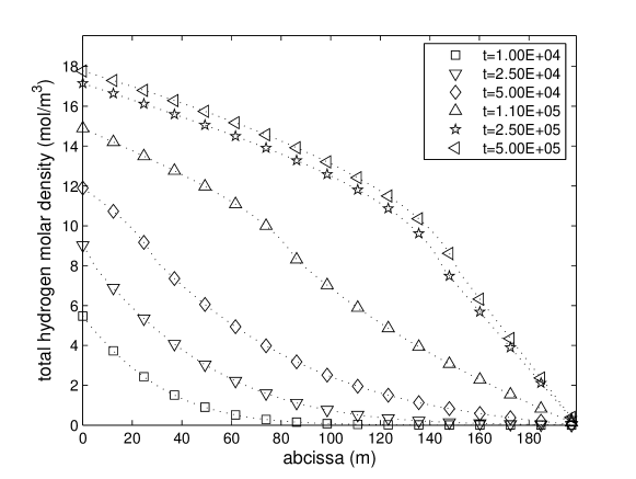
Figure 1: Test case 1 : spatial evolution along the line ${\cal L}_{cut}$ of the total hydrogen molar density $\frac{\rho_{g}^{std}}{M^{h}}X$ at several times $t$ (in years)

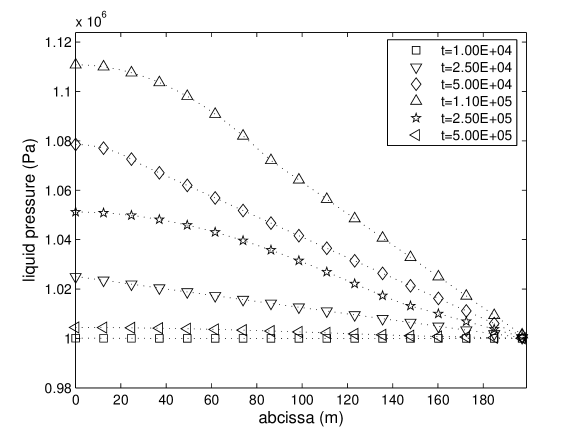
Figure 2: Test case 1 : spatial evolution along the line ${\cal L}_{cut}$ of the liquid pressure $p_{l}$ at several times $t$ (in years)

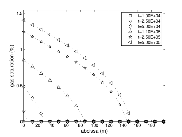
Figure 3: Test case 1 : spatial evolution along the line ${\cal L}_{cut}$ of the gas saturation $S_{g}$ at several times $t$ (in years)

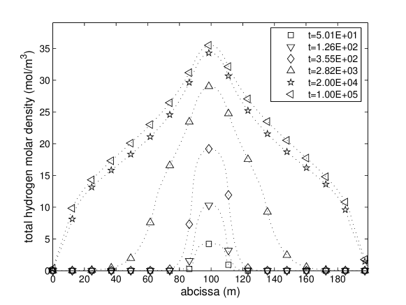
Figure 4: Test case 2 : spatial evolution along the line ${\cal L}_{cut}$ of the total hydrogen molar density $\frac{\rho_{g}^{std}}{M^{h}}X$ at several times $t$ (in years)

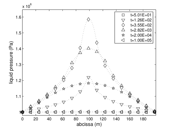
Figure 5: Test case 2 : spatial evolution along the line ${\cal L}_{cut}$ of the liquid pressure $p_{l}$ at several times $t$ (in years)

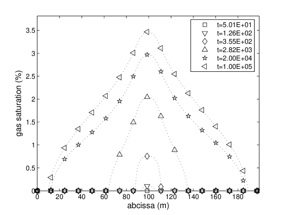
Figure 6: Test case 2 : spatial evolution along the line ${\cal L}_{cut}$ of the gas saturation $S_{g}$ at several times $t$ (in years)

4 Concluding remarks

From balance equations, constitutive relations and equations of state, assuming thermodynamical equilibrium, we have derived a model for describing underground gas migration in water saturated or unsaturated porous media, including diffusion of components in phases and capillary effects. In the last part of this paper, numerical simulations on simplified situations inspired by the ”Couplex-gas” benchmark Bench , show evidence of its ability : - to describe gas (hydrogen) generation and migration - and to treat the difficult problem, as it appeared in the results of ”Couplex-gas” Bench , of correctly simulating evolution of the unsaturated region, in a deep geological repository, created by gas generation. A forthcoming paper will be devoted to the use of this model for solving the ”Couplex-gas” benchmark Bench and other 3-D situations of gas migration in water saturated or unsaturated porous media, including the design a of numerical test cases synthesizing the main challenges appearing in gas generation and migration.

References

• (1) Myron B. Allen III: Numerical Modelling of Multiphase Flow in Porous Media, Adv. Water Resources, 8, 162-187 (1985).
• (2) Jacob Bear and Yechuda Bachmat: Introduction to Modeling of Transport Phenomena in Porous Media, Kluwer, Dordrecht, 1991.
• (3) Guy Chavent and Jérôme Jaffré: Mathematical Models and Finite Elements for Reservoir Simulation, North-Holland, 1986.
• (4) Abbas Firoozabadi: Thermodynamics of Hydrocarbon Reservoirs, McGraw-Hill, New York, 1999.
• (5) Horseman,S.T., Higgo,J.J.W., Alexander, J., Harrington,J.F., Water, gas and solute movement through argillaceous media, NEA Report CC-96/1, Paris, OECD, 1996.
• (6) Jin Y, Jury W.A., Characterizing the dependence of gas diffusion coefficient on soil properties. Soil Sci. Soc. Am. J., 60, 66-71.
• (7) C.M. Marle, Multiphase Flow in Porous Media, Édition Technip, 1981.
• (8) Millington R.J., Shearer R.C., Diffusion in aggregated porous media. Soil Science Vol. 111. NO. 6, 372, 1971
• (9) D.W. Peaceman, Fundamentals of numerical reservoir simulation, Elsevier, Amsterdam, 1977.
• (10) Pruess K.,Oldenburg C. and Moridis G., Tough2 User’s Guide, version 2.0., Lawrence Berkeley National Laboratory, Berkeley, 1999.
• (11) Schlumberger ECLIPSE Technical Description 2005 A, Schlumberger.
• (12) Van Genuchten, M. (1980). A closed form equation for predicting the hydraulic conductivity of unsaturated soils. Soil Sci. Soc. Am. J. 44, 892-898.
• (13) Mualem, Y. (1976). A New Model for Predicting the Hydraulic Conductivity of Unsaturated Porous Media. Water Resour. Res. 12(3), 513 522.
• (14) Andra, Couplex-gaz,
http://www.andra.fr/interne.php3?id_article=913&id_rubrique=76
• (15) CEA, Cast3m,
http://www-cast3m.cea.fr/cast3m/index.jsp