Heat conduction in simple networks: Controlling heat flow through inter-chain coupling

Abstract

The heat conduction in simple networks consisting of different one dimensional nonlinear chains is studied. We find that the coupling between chains has different function in heat conduction compared with that in electric current. This might find application in controlling heat flow in complex networks.

Energy and information transports on networks, such as the metabolism network, neuronal network, porous material network, and oil production network, etc., have been studied for a long time Stauffer:1992 and is recently getting more attention because of the hectic activity in the complex networks and the great progress in nanoscale fabrication technology where the naotube/nanowire networks can be made for different purposes Yakov:2004 ; Kumar:2005 ; Chub:2005 ; Lopez:2005 ; Wu:2005 ; Lizana:2005 ; Albert:2002 . It is found that the electric transport changes linearly with the number of added bonds Chub:2005 ; Kumar:2005 . The whole resistance of network can be figured out by the Kirchhoff second law for the complicated parallel and serial electric circuit Lopez:2005 .

However, little is known about heat conduction in the complex networks, although some progress has been achieved in the study of heat conduction in single one dimensional chains (See Ref.Review and the references therein). The fundamental question for heat conduction in one dimensional chains is that what is the necessary and/or sufficient condition for the heat conduction to obey the Fourier law. From computer simulations, it is found that in 1D nonlinear lattices with on-site potential such as the Frenkel-Kontorova (FK) model and the $\phi^{4}$ model, the heat conduction obeys the Fourier’s law, namely, the heat conductivity is size independentFK , which is also called normal heat conduction. Whereas in other nonlinear lattices without on-site potential, thus momentum is conserved, such as the Fermi-Pasta-Ulam (FPU) and alike models, the heat conduction exhibits anomalous behaviorFPU , namely the heat conductivity $\kappa$ diverges with the system size $N$ as $\kappa\sim N^{\delta}$. A great effort has been devoted to understand the physical origin and the value of the divergent exponent $\delta$Exponent . It is found that the anomalous heat conduction is due to the anomalous diffusion and a quantitative connection between them has been establishedLi . Most recently, we found that both the normal and anomalous heat conduction can be described by an effective phonon theory under the same frameworkLTL .

More importantly, it is found that a single 1D chain consists of two different lattices exhibit very interesting physical phenomena such as thermal rectificationDiode and negative differential thermal resistanceLWC2 . Experimental on nanotube has verified the rectification Berkely . Opening up a new field of controlling heat flow from simple (or complex) nano scale networks.

All studies on the 1D single chain can be regarded as the first step to understand the heat conduction on realistic situations, i.e., complex networks. In general, a complex network consists of many 1D (or quasi-1D) chains with a diversity of couplings among them. Therefore, the key to understand the heat conduction on networks is to understand the influence of coupling to heat fluxes in simple networks, i.e., coupled chains. According to the best of our knowledge, this problem has not been investigated so far.

For the sake of simplicity, we would like to consider $m$ 1D chains with several couplings between any two of them. To be more specific, we take the FPU-$\beta$ chainFPU as the basic element and each chain are contacted with the Nose-Hoover thermostat Nose:1984 at the two ends, keeping the first and the last particle of the chain at temperature $T_{h}$ and $T_{l}$, respectively. Without coupling, each chain has a Hamiltonian $H=\sum_{i}\frac{1}{2}p_{i}^{2}+V(x_{i},x_{i+1})$, where $V(x_{i},x_{i+1})=\frac{1}{2}\sum_{i}(x_{i+1}-x_{i})^{2}+\frac{1}{4}\sum_{i}(x_{i+1}-x_{i})^{4}$, $x_{i}$ represents the displacement from the equilibrium position of the i’th particle. The motion of the particles for $i=2,3,\cdots,N-1$ satisfy the canonical equations $\dot{x_{i}}=\frac{\partial H}{\partial p_{i}}$; $\dot{p_{i}}=-\frac{\partial H}{\partial x_{i}}$. The dynamical equations for the heat baths are $\dot{\xi}_{h}=\frac{\dot{x}_{1}^{2}}{T_{h}}-1,\dot{\xi}_{l}=\frac{\dot{x}_{N}^{2}}{T_{l}}-1$. The dynamical equations for the first and last particles are $\dot{p}_{1}=-\frac{\partial H}{\partial x_{1}}-\xi_{h}p_{1}$, $\dot{p}_{N}=-\frac{\partial H}{\partial x_{N}}-\xi_{l}p_{N}$.

The temperature is defined as $T(i)=\langle p_{i}^{2}\rangle$ and the heat flux along the chain is $J=\langle p_{i}\frac{\partial V}{\partial x_{i+1}}\rangle$. Suppose there is a coupling between the node $i$ of one chain and the node $j$ of another chain, then we have an additional new potential $V_{ij}^{\prime}=\frac{1}{2}(x_{i}-x_{j})^{2}+\frac{1}{4}(x_{i}-x_{j})^{4}$. The equations of node $i$ and node $j$ become

$$\dot{p_{i}}=-\frac{\partial H}{\partial x_{i}}-\frac{\partial V_{ij}^{\prime}}{\partial x_{i}};\dot{p_{j}}=-\frac{\partial H}{\partial x_{j}}-\frac{\partial V_{ij}^{\prime}}{\partial x_{j}}.$$ (1)

To investigate the influence of coupling by numerical simulations, we take $T_{h}=0.7$ and $T_{l}=0.5$ for all the chains and first consider the case of $m=2$, i.e., two coupled chains in this Letter. The two chains are coupled at different nodes $i,j$. We find that both the temperature distribution and the total flux in the steady state are changed with the coupling positions.

Case I: two chains of the same length coupled together

The two chains are identical of length $N=20$. Like all models of heat conduction, there are always temperature jumps at the two boundariesJump as is clearly shown in Fig. 1. When two chains are coupled together regardless of the coupling position, there is also temperature jump at the junction, see Fig. 1(b)-(d).

In Fig. 2 where we shows the corresponding fluxes of Fig. 1 where the arrows denote the directions of fluxes. Fig. 2(a) is easy to understand from their identity, where two uncoupled chains have the same flux.

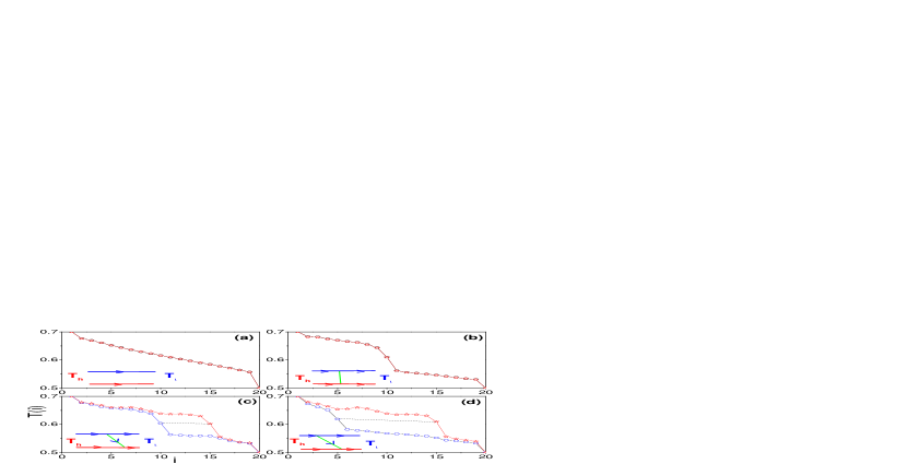
Figure 1: Temperature distributions of two coupled chains of length $N=20$ with different coupling positions. The thin lines (green) denote the coupling. The insets are the schematic configurations of coupled chains, and the arrows there label the direction of heat flow. (a) No coupling, (b) Coupling at $i=j=10$. (c) Coupling at $i=10,j=15$. (d) Coupling at $i=5,j=15$.

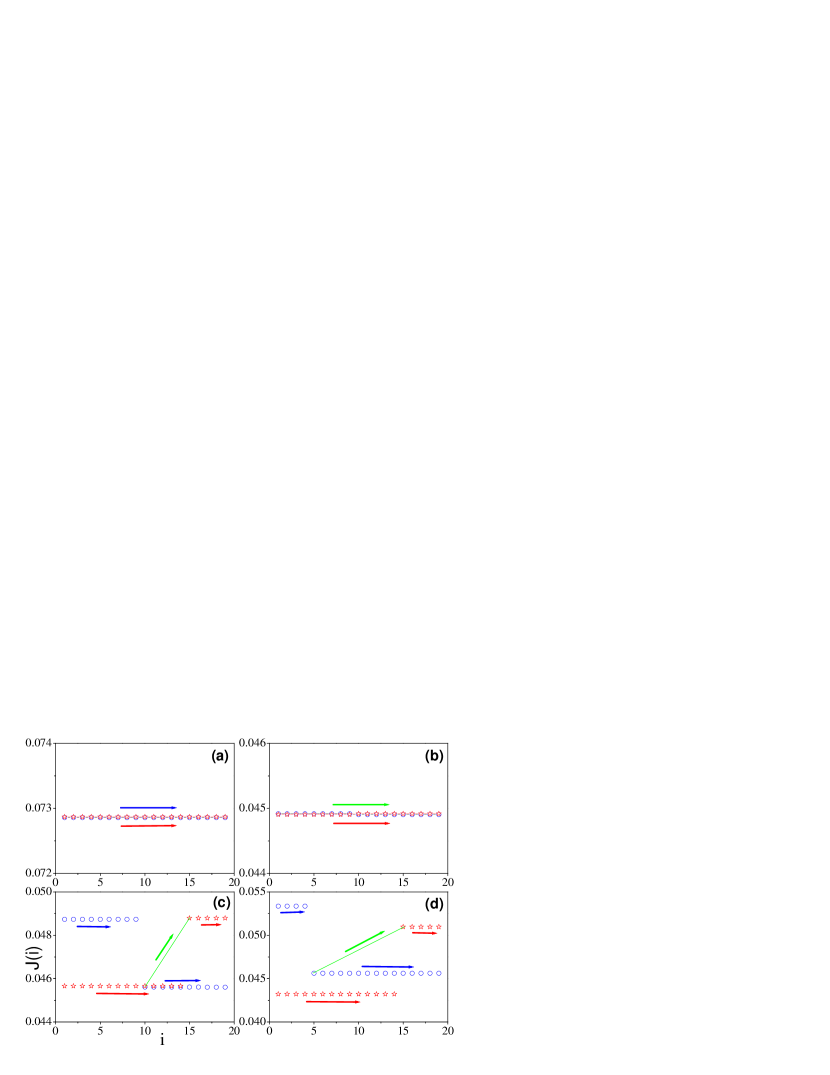
Figure 2: The corresponding fluxes of Fig. 1.

Fig. 2(b) shows a very interesting result - the reduction of the heat current. This is completely different from electric circuit. It is well known that a circuit of two chains with four equal resistance R connected by a conduction line at the middle is a symmetric circuit. Since there is no potential difference between the two connecting points, there is no current through the middle connection line, thus the current in the circuit does not change! It remains the same if the two chains are disconnected.

What makes the ”thermal circuit” different from the electric circuit? To this end, we need to go to the definition of temperature. The temperature is a measure of the kinetics of the particle. It is an ensemble (time) average of the kinetic energy. Without coupling, the middle particle at each chain is connected only by its two nearest neighbors. After coupling, the middle particle is connected with three particles which changes its equation of motion. Even though the two particles in the middle have the same temperature (same average kinetic energy and same velocity distribution), it does not mean that the two particles always oscillate in the same way. This is the fundamental difference between the electric circuit and thermal circuit.

In fact, the coupling of the second chain to the first chain is equivalent to the introduction of an interface resistance at the junction. This resistance is also called the Kapitza resistance which is defined as: $R_{int}=\Delta T/J$, where the $\Delta T$ is the temperature jump between the left and right particles of the interface (coupled particle in the middle). Therefore the heat current through each chain is:

$$J=\frac{T_{h}-T_{l}}{2R+R_{int}}$$ (2)

which is obviously less than $J_{0}=\frac{T_{h}-T_{l}}{2R}$ for the uncoupled chain.

In the case of without any coupling, the temperature of the $i^{\prime}th$ particle inside the FPU chain is:

$$T_{i}\approx T_{h}-|\Delta T_{h}|-\frac{i-1}{N-2}\left(T_{h}-|\Delta T_{h}|-T_{l}-|\Delta T_{l}|\right),$$ (3)

where $|\Delta T_{h}|$ and $|\Delta T_{l}|$ is the temperature jump at the both ends between the heat bath and the first/last particle of the chain, respectively. The heat current flows at the junction can be understood from this formula. For instance, the particle at $i=10$, has higher temperature than the particle of $i=15$. Heat flows always from high temperature to low temperature, therefore, if one connects $i=10$ in upper chain to particle $i=15$ in lower chain, there will be heat current flows from $i=10$ (higher temperature) in upper chain to particle $i=15$ (low temperature) in the lower chain. This will drag the temperature of particle $i=10$ down a little bit, thus we see the increase of the heat current in the part of $i\in[2,10]$ in upper chain in Fig. 2(c) compared with the case in Fig. 2(b). In contrast, as the heat current flows to particle $i=15$ at lower chain, the temperature at $i=15$ is increased, thus the increase of the temperature difference between $i=15$ and $i=20$, which leads to the increase of heat current in segment of $i\in[15,20]$ in lower chain. This is what we observe in Fig. 1 (c). The same mechanism applies also to Fig 1 (d).

Case II: Two chains of different length coupled together

We would like to extend above ideas to more general case, namely, coupling of two chains of different length and multiple coupling. We find that the reduction of heat flux by coupling is quite general. Fig. 3 shows the temperature distribution of two coupled chains with different lengthes $N_{1}=20$ and $N_{2}=30$, respectively. (See Figure caption for more information.) It is easy to see that Fig. 3 has some similarity with Fig. 1, i.e., there are temperature jumps at the coupled particles and the coupled particles have the approximate same temperature.

Another interesting thing is that the crossing couplings make the middle part of the coupled chains appear a temperature plateau which might be useful in heat control.

Fig. 4 shows the corresponding fluxes of Fig. 3. The longer chain, $N_{2}=30$ has smaller heat current. Although the coupling of the two chains of different length is not at the symmetrical point, there is still no current through the coupling.

In fact, the like in the previous case shown in Fig. (1) and (2), the heat current flow in the (multi) coupled chain of different length can be also understood from Eq. (3). According to this formula, we can roughly estimate that the $T_{5}$ at short chain is roughly the same as $T_{8}$ in the longer chain. Thus there is no heat flow between them. The only influence is the introduction of an interface resistance which drags down the heat current through each chain as is seen in Fig. 3(b).

It is not difficult to estimate that $T_{5}$ at chain $N=30$ is larger than $T_{5}$ at chain $N=30$. This is why we see the current flow from particle 5 at lower (longer) chain to particle 5 at upper (shorter) chain in Fig. 4. However, the temperature of particle 15 at upper chain (shorter) is almost the same as the temperature of particle 25 at lower chain (longer) if the two chains are uncoupled. However, due to first coupling, the temperature of particle 15 at upper chain is slightly increased, this is why we see the current flows from particle 15 in upper chain to the particle 25 in low chain as shown in Fig 4(c).

More complicated and more interesting case is shown in Fig. 4(d), where we have two crossing couplings: $i_{1}=5$ is connected to $i_{2}=15$, and $j_{1}=20$ is connected to $j_{2}=10$. Use Eq.(3), we can again estimate that $T_{i_{1}=5}>T_{i_{2}=15}$, thus we see the current flow from upper chain to the lower chain. Similarly, there is heat current flows from lower chain (particle $j_{2}=10$) to upper chain ($j_{1}=20$).

We have also checked the heat conduction in multiple coupled chains with a diversity of couplings, such as in the three coupled chains with different lengthes, and observed the similar results as in the case of two coupled chains. We conclude that, in general, the coupling will introduce an interface resistance at the junction thus affect the heat flow through the whole system.

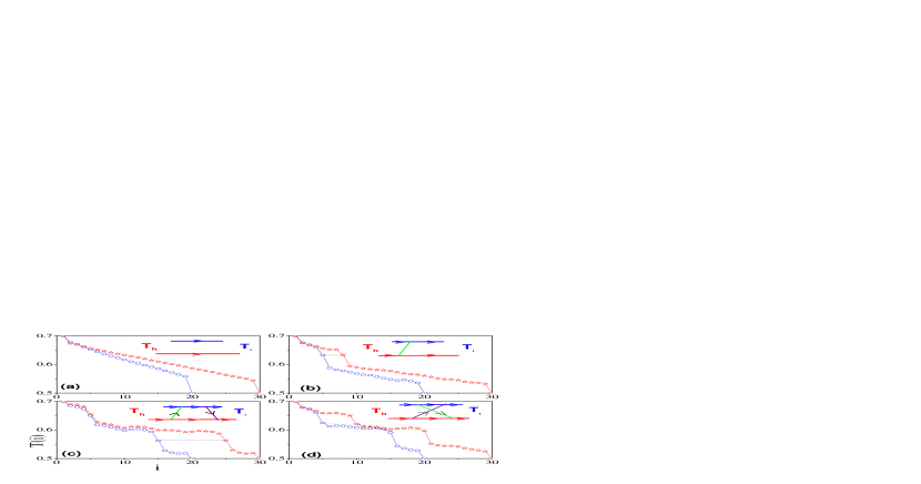
Figure 3: Temperature distributions of two coupled chains with different lengthes $N_{1}=20$ and $N_{2}=30$ with different coupling positions. The thin (green and purple) lines denote the coupling. The insets are the schematic configurations of coupling chains, and the arrows indicate the direction of heat flow. (a) no coupling, (b) one coupling added at $i=5,j=8$; (c) two couplings added at $i_{1}=5,j_{1}=5$ and $i_{2}=15,j_{2}=25$; (d) two crossing couplings added at $i_{1}=5,j_{1}=20$ and $i_{2}=15,j_{2}=10$.

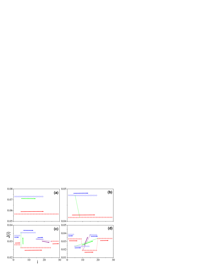
Figure 4: The corresponding fluxes of Fig. 3.

Case III: Single chain with loop

Another interesting question is how the self-coupling or a shortcut in a single chain affect the heat current? This case happens very frequently in the polymer chain and biological systems???. For example, if there is a shortcut between the node $i$ and the node $j$ of a chain (see the inset of Fig. 5(a)), does this shortcut reduce the flux of the chain? In the case of traffic flow (reference ????), the shortcut increases the capacity of traffic because the vehicles have more free space to go. However, in the thermal circuit, the flux should be reduced because of the interface resistance. The line with “stars” in Fig. 5(b) shows the result with $N=20,i=5$, and $j=15$. Comparing it with Fig. 2(a) of no coupling, it is easy to see that the flux is reduced almost $50\%$.

We also study the dependence of the reduction of the heat flux on the coupling strength $k$. From the definition of junction resistance we know that the larger the degree of destroying the correlation between the coupled particle and its neighbors is, the larger $R_{int}$, i.e., $R_{int}$ should monotonously increase with $k$. When the correlation is completely destroyed, $R_{int}$ cannot be increased more by further increasing $k$. Therefore, there is a saturation effect for $R_{int}$ and the effect of junction resistance when $k$ is large enough. Let’s confirm this prediction by numerical simulations. In this situation, the coupling potential becomes

$$V_{ij}^{\prime}=\frac{k}{2}(x_{i}-x_{j})^{2}+\frac{k}{4}(x_{i}-x_{j})^{4}.$$ (4)

Substituting Eq. (4) into Eq. (1) we get the dynamical equations for the particles with coupling strength $k$. Our numerical simulations show that for a single chain with the self-coupling, the larger the coupling is, the more reduction of flux. Fig. 5(b) shows three typical cases where the lines with “circles”, “stars” and “squares” denote the cases of $k=0.5$ and $2.0$, respectively. From the middle parts of this figure it is ease to see that the larger coupling makes less flux go through the original path. We notice that the coupling also changes the temperature distribution. The strong the coupling is, the two particles connected by the coupling have more close temperatures, as shown in Fig. 5(a). For observing the influence of coupling strength in more detail, Fig. 5(c) shows how the fluxes change with the coupling strength $k$ where the line with “circles” denotes the total flux and the line with “stars” the flux going through the shortcut. Obviously, the total flux becomes stabilized when $k>1$ and the flux through the shortcut is monotonously increase with $k$, confirming the saturation effect. The saturation effect has been also observed in the coupling of two coupled chains, see Fig. 5(d) for how the total flux of the two chains in Fig. 2(b) changes with the coupling strength $k$.

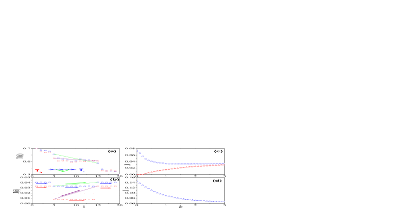
Figure 5: (a) and (b) represent the distributions of temperature and flux in a single chain with $N=20,i=5$ and $j=15$, respectively, where “circles” and “squares” denote the cases of $k=0.5$ and $2.0$, respectively. The arrows in the inset of (a) indicate the direction of heat flow. (c) shows how the flux in (b) changes with the coupling strength $k$ where the “solid square” are the total flux and the “open circle” the flux through the shortcut. (d) The heat current in Fig. 2(b) changes with the coupling strength $k$.

In conclusions, we have studied the influence coupling in simple networks on the heat conduction. It is found that different from the electric circuit, the coupling affect very much the heat current flow in the thermal circuit. Any introduction of coupling is equivalent to an introduction of an interface resistance, thus influence largely the heat current in the circuit. The study may shed lights for studying heat conduction in complex networks.

ZL is supported in part by the NNSF of China under Grant No. 10475027 and No. 10635040, by the PPS under Grant No. 05PJ14036, by SPS under Grant No. 05SG27, and by NCET-05-0424. BL is supported partially by a FRG grant and a ARF grant.

References

- (1) D. Stauffer and A. Aharony, Introduction to percolation Theory Taylor Francis, London, 1992.
- (2) Y. M. Syrelniker, R. Berkovits, A. Frydman, and S. Havlin, Phys. Rev. E 69, 065105(R) (2004).
- (3) S. Kumar, J. Y. Murthy, and M. A. Alam, Phys. Rev. Lett. 95, 066802 (2005).
- (4) M. V. Chubynsky and M. F. Thorpe, Phys. Rev. E 71, 056105 (2005).
- (5) E. Lopez, S. V. Buldyrez, S. Havlin, and H. E. Stanley, Phys. Rev. Lett. 94, 248701 (2005).
- (6) Z. Wu et al., Phys. Rev. E 71, 045101(R) (2005).
- (7) L. Lizana and Z. Konkoli, Phys. Rev. E 72, 026305 (2005).
- (8) R. Albert and A.-L. Barabasi, Rev. Mod. Phys. 74, 47(2002).
- (9) F. Bonetto et al., in Mathematical Physics 2000, edited by A. Fokas et al. (Imperial College Press, London, 2000), p.128.
- (10) B. Hu, B. Li and H. Zhao, Phys. Rev. E 57, 2992 (1998); Phys. Rev. E 61, 3828 (2000); K. Aoki and D. Kusnezov, Phys. Lett. A 265, 250 (2000).
- (11) H. Kaburaki and M. Machida, Phys. Lett. A 181, 85 (1993); A. Fillipov, B. Hu, B. Li, and A. Zeltser, J. Phys. A 31. 7719 (1998); K. Aoki and D. Kusnezov, Phys. Rev. Lett 86, 4029 (2001).
- (12) A. Pereverzev, Phys. Rev. E 68, 056124 (2003);O. Narayan and S. Ramaswamy, Phys. Rev. Lett. 89, 200601 (2002); J.-S Wang and B Li, Phys. Rev. Lett, 92, 074302 (2004); Phys. Rev. E 70, 021204 (2004).
- (13) B. Li and J. Wang, Phys. Rev. Lett. 91, 044301 (2003); 92, 089402 (2004); B. Li, J. Wang, L. Wang and G. Zhang, Chaos 15, 015121 (2005).
- (14) N. Li, P. Tong and B. Li, Europhys. Lett. 75, 49 (2006).
- (15) B. Li, L. Wang and G. Casati, Phys. Rev. Lett. 93, 184301 (2004); B. Li, J. Lan and L. Wang, Phys. Rev. Lett. 95, 104302 (2005); B. Hu, L. Yang, and Y. Zhang, Phys. Rev. Lett. 97, 124302 (2006); J.-H Lan and B. Li, Phys. Rev. B 74, 214305 (2006).
- (16) B. Li, L. Wang and G. Casati, Appl. Phys. Lett. 88, 143501 (2006).
- (17) C. W. Chang, D. Okawa, A. Majumdar and A. Zettl, Science 314, 1121 (2006).
- (18) S. Nose, J. Chem. Phys. 81, 511 (1984); W. G. Hoover, Phys. Rev. A 31, 1695 (1985).
- (19) K. Aoki and D. Kusnezov, Phys. Rev. Lett. 86, 4029 (2001).
- (20) C. Maes, K. Netocny, and M. Verschuere, J. Stat. Phys. 111, 1219 (2003).
- (21) J.-P. Eckmann and E. Zabey, J. Stat. Phys. 114, 515 (2004).
- (22) Z. Rieder, J. L. Lebowitz, and E. Lieb, J. Math. Phys. (N. Y.) 8, 1073 (1967).