BOUND STATE INEQUALITY FOR HIGH MASS EXCHANGES IN A SCALAR FIELD MODEL

Abstract

Ladder diagrams are relevant for the study of bound states. The condition upon the coupling strength for the existence of a bound state has been deduced in a scalar field theory for the case of low mass exchanges. We apply this approach to the case of very high mass exchanges.

03.65.Nk, 03.70.+k, 11.10.St (pacs).

I. INTRODUCTION

A fundamental question in quantum mechanics is the existence, spectrum and properties of bound states[1, 2, 3, 4]. The importance of this subject matter for atomic and molecular physics is obvious. In particle physics it is also of primary importance. Positronium, heavy quark bound states such as $J/\psi$ and indeed all quark (anti-quark) bound states are of interest to physicists and often provide information about constituent roles and theoretical models. Resonances are a related subject matter but unlike bound states they are above threshold and have finite lifetimes either because they decay via a weaker interaction, such as for the flavor changing quark decays, or because they are “excited” states that eventually de-excite to the ground state[2].

The main approach to bound states has been the solution of the appropriate non-relativistic wave equation in the presence of a potential[2, 3, 4]. This is perfectly adequate when the solutions yield non-relativistic bound states. For better precision, their relativistic corrections can be treated with equations such as the Dirac or Klein-Gordon equations. However, these relativistic equations exhibit one very important limitation[5] when used for calculating bound states, related to the Klein paradox[6, 7, 8, 9, 10].

For long range interactions, such as electromagnetic or gravitational, an infinite number of bound states exist. For short range interactions such as that given by a Yukawa potential,

$$V_{\mbox{\tiny Y}}(r)=-\,\frac{g_{\mbox{\tiny eff}}^{\mbox{\tiny$2$}}}{4\,\pi}\,\frac{\exp[-\,\mu\,r]}{r}\,\,,$$ (1)

corresponding to the exchange of a particle of mass $\mu$, only a finite number of bound states exist if any at all. Indeed for small mass exchanges (compared to the systems reduced mass), numerical calculations within the Schrödinger equation yield a minimum condition for the existence of a bound state, i.e.

$$\frac{g^{\mbox{\tiny$2$}}_{\mbox{\tiny eff}}}{4\,\pi}\geq 0.84\,\frac{\mu}{m}\,\,,$$ (2)

where $\mu$ is the exchanged particle mass and $m$ is the reduced mass. To the extent that this inequality is valid, i.e. that the potential is realistic and that the Schrödinger equation is acceptable, it tells us that as the range of the interaction falls ($\mu$ and hence $\mu/m$ increases) the coupling strength must grow as $\mu/m$ to permit the existence of a bound state. However, as the coupling grows so does, in general, the binding energy, $E_{b}$. For example, in the Bohr model $E_{b}\propto\alpha^{\mbox{\tiny$2$}}$, with $\alpha\equiv g^{\mbox{\tiny$2$}}_{\mbox{\tiny eff}}/4\,\pi$, so that eventually the Schrödinger equation becomes inappropriate as the binding energy tends to or exceeds the reduced mass.

If one considers a potential which is akin to the Yukawa potential but has the advantage of being solvable exactly[11], i.e. the Hulthen potential

$$V_{\mbox{\tiny H}}=-\,\frac{g_{\mbox{\tiny eff}}^{\mbox{\tiny$2$}}}{4\,\pi}\,\frac{2\,\mu}{\exp[2\,\mu\,r]-1}\,\,,$$ (3)

one finds, analytically, the condition for the single (s-wave) bound state to exist to be similar to the numerically inequality found in Eq.(2), i.e.,

$$\frac{g^{\mbox{\tiny$2$}}_{\mbox{\tiny eff}}}{4\,\pi}\geq\frac{\mu}{m}\,\,.$$ (4)

For completeness, we should point out that there is a whole class of Hulthen potentials with $\mu$ in the above expression substituted by $c\,\mu$ (where $c$ is a positive constant). Our particular choice ($c=1$) is that which shares with the Yukawa (mass $\mu$) the same first two terms in a Maclaurin series expansion about $r=0$.

Relativistic spinor bound states, by which we mean any spinor bound states for which relativity plays an important role, require more care. We can first attempt to treat these states by including the lowest order relativistic corrections to the Schrödinger equation or by passing directly to the Dirac equation[1, 2, 3, 4] . In either of these cases, one can demonstrate that as $\mu$ increases relativistic effects automatically increase the effective coupling constant. We have called this effect the amplification of the Yukawa coupling[5]. This opens the practical possibility of high mass exchange bound states. However, if the bound state energy grows with the effective coupling constant, as numerical calculations suggest, then we will eventual enter the so-called Klein zone $E<V_{\mbox{\tiny$0$}}-m$. Conventionally $V_{\mbox{\tiny$0$}}$, which is the asymptotic free space value, is set to zero. Within the Klein zone only oscillatory solutions exist everywhere. This is the origin of the Klein paradox which can be interpreted as a consequence of pair creation[6, 7, 8, 9, 10]. This is a positive feature, if considered an anticipation of field theory, but it is a problem for the one-particle interpretation of these equations. Furthermore, the absence of evanescent solutions means the absence of any (discrete spectrum) bound states.

At this point, one naturally passes to field theory. This seems promising since one of the greatest successes of renormalized field theory is the calculation of the Lamb shift[12]. Unfortunately the very existence of a bound state, while a more elementary question, seems much more difficult to answer in field theory. This is the reason that one often falls back upon (heuristic) two-body relativistic equations, albeit inspired by field theory, such as the Bethe-Salpeter equation[13, 14, 15], the Blankenbecler-Sugar equation[16] or the Gross (spectator) equation[4]. There is however one technique, described in detail by Franz Gross[17], which offers us a very useful tool. This is based upon the sole consideration of ladder diagrams and works impressively for small $\mu/m$. Indeed, after introduction of the scalar model in the next section, we present in section III a simplified (zero momentum) calculation (for light mass exchanges) which exactly reproduces the Hulthen inequality. In section IV, we consider the opposite limit where $\mu/m$ is very large. We seek the appropriate inequality condition for the existence of a bound state for this limit and, with the help of some numerical calculations, this will indeed be found.

The reasons for our interest in this high mass exchange limit is that some physical interactions do indeed involve very heavy mass exchanges[2], e.g. the exchange of of the intermediate vector bosons $W^{\pm}$ and $Z^{\mbox{\tiny$0$}}$, and almost certainly of the Higgs particle. In particular, since the neutrino is now known to have mass eigenstates[18], it is a legitimate question to ask if the weak interactions allow for, say, neutrino-lepton bound states[5]. The above inequalities suggests not, for we are asking if a bound state can exist with a $\mu/m$ ratio $>10^{10}$ for neutrino-electrons (although this ratio could be much smaller for the heavier leptonic families). However, these inequalities have been derived from non-relativistic equations or, as we shall see, from ladder diagrams in which the assumption of small $\mu/m$ is made from the start. We shall return briefly to this discussion in our conclusions.

II. THE SCALAR MODEL

Let us consider a scalar model with three different mass scalars. Two of them represent the incoming system and have mass $m_{\mbox{\tiny$1$}}$ and $m_{\mbox{\tiny$2$}}$. They interact only by the exchange of a third scalar with mass $\mu$. The dimensional coupling constants are $\lambda_{\mbox{\tiny$1$}}$ and $\lambda_{\mbox{\tiny$2$}}$ for the particle with mass $m_{\mbox{\tiny$1$}}$ and $m_{\mbox{\tiny$2$}}$ respectively. The one boson exchange diagram gives the lowest order contribution to the invariant scattering amplitude,

$$\mathcal{M}_{\mbox{\tiny tree}}(q)=i\,(-\,i\,\lambda_{\mbox{\tiny$1$}})\,(-\,i\,\lambda_{\mbox{\tiny$2$}})\,\frac{-\,i}{\mu^{\mbox{\tiny$2$}}-q^{\mbox{\tiny$2$}}-i\,\epsilon}=-\,\frac{\lambda_{\mbox{\tiny$1$}}\lambda_{\mbox{\tiny$2$}}}{\mu^{\mbox{\tiny$2$}}-q^{\mbox{\tiny$2$}}-i\,\epsilon}\,\,.$$ (5)

From the Fourier transform of Eq.(5) when $q_{\mbox{\tiny$0$}}=0$ one obtains the Yukawa potential quoted above. The corresponding force is attractive (and hence can yield bound states) only if $\lambda_{\mbox{\tiny$1$}}\lambda_{\mbox{\tiny$2$}}>0$. In fact, comparing with the attractive Yukawa shows that

$$g_{\mbox{\tiny eff}}^{\mbox{\tiny$2$}}=\frac{\lambda_{\mbox{\tiny$1$}}\lambda_{\mbox{\tiny$2$}}}{4\,m_{\mbox{\tiny$1$}}\,m_{\mbox{\tiny$2$}}}\,\,.$$ (6)

Henceforth this is what we shall assume throughout. The scattering amplitude reduces to a number for forward scattering,

$$\mathcal{M}_{\mbox{\tiny tree}}(0)=-\,\frac{\lambda_{\mbox{\tiny$1$}}\lambda_{\mbox{\tiny$2$}}}{\mu^{\mbox{\tiny$2$}}}\,\,.$$ (7)

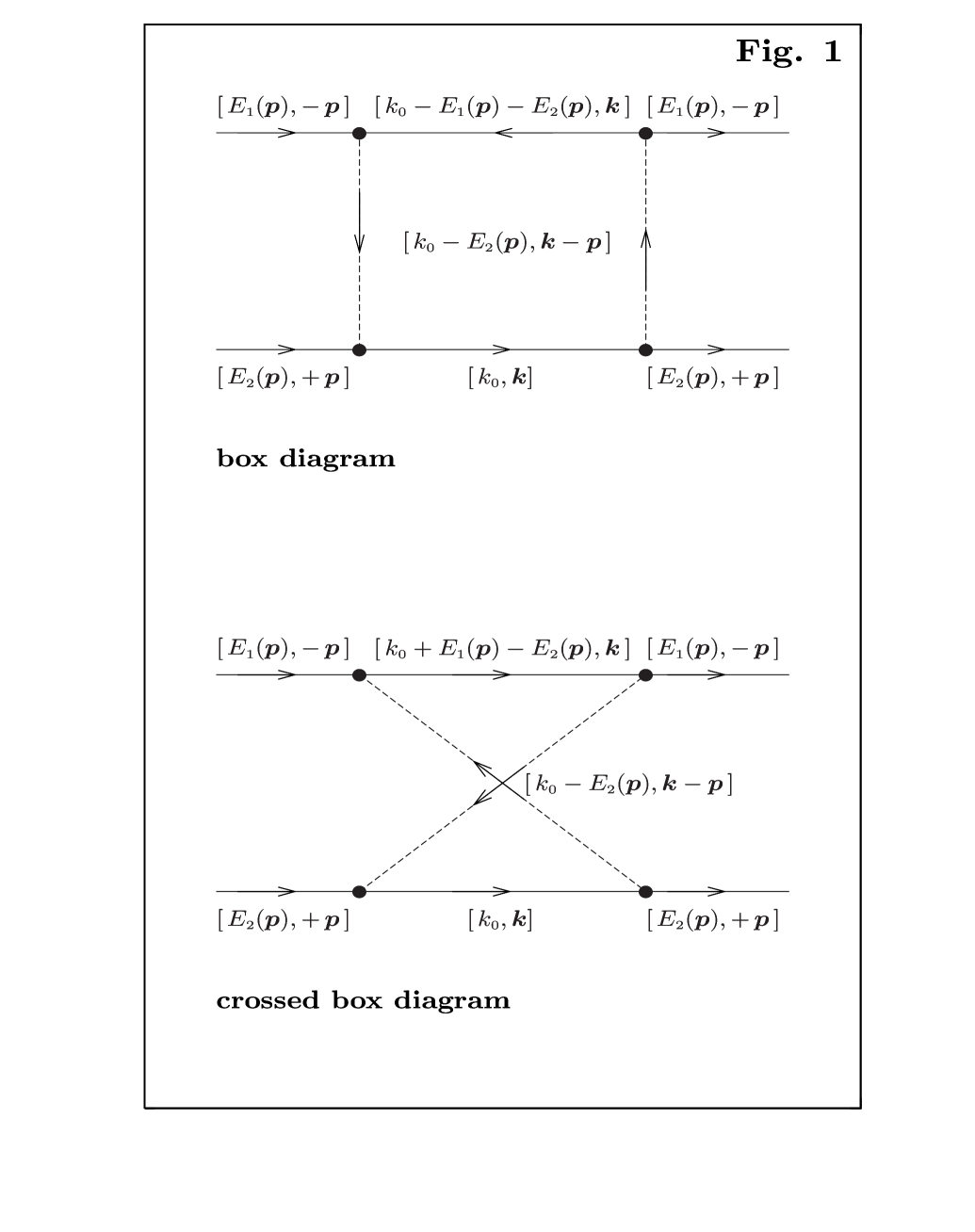
Figure 1: The fourth order box and crossed box diagrams in a scalar field model evaluated in the center of mass frame for scattering in the forward direction.

The fourth order ladder and crossed (ladder) diagrams are shown in Fig. 1. Not surprisingly, these contributions modify the Yukawa potential as do all higher order terms. We shall come back to this discussion in the next section. The box and crossed box diagrams are not the only fourth order diagrams, but the others can be absorbed into the dressing of the propagators and vertex functions. As a consequence of the latter, we expect the appearance of form factors which however reduce to unity for forward scattering. For our purposes it is sufficient to limit our calculations to forward scattering. Consequently, we will not consider explicitly these other diagrams [4].

In the center of mass system and for forward scattering (see Fig. 1), the Feynman rules for the box diagram amplitude yield

$$\mathcal{M}^{\square}=i\,\lambda_{\mbox{\tiny$1$}}^{\mbox{\tiny$2$}}\lambda_{\mbox{\tiny$2$}}^{\mbox{\tiny$2$}}\int\frac{\mbox{d}^{\mbox{\tiny$4$}}k}{(2\pi)^{\mbox{\tiny$4$}}}\,\frac{1}{D_{\mbox{\tiny$1$}}D_{\mbox{\tiny$2$}}D^{{}^{\mbox{\tiny$2$}}}_{\mbox{\tiny$0$}}}$$ (8)

with

$$D_{\mbox{\tiny$1$}} = \left[\,E_{\mbox{\tiny$1$}}(\boldsymbol{k})-E_{\mbox{\tiny$1$}}(\boldsymbol{p})-E_{\mbox{\tiny$2$}}(\boldsymbol{p})+k_{\mbox{\tiny$0$}}-i\epsilon\right]\,\left[\,E_{\mbox{\tiny$1$}}(\boldsymbol{k})+E_{\mbox{\tiny$1$}}(\boldsymbol{p})+E_{\mbox{\tiny$2$}}(\boldsymbol{p})-k_{\mbox{\tiny$0$}}-i\epsilon\right]\,\,,$$

$$D_{\mbox{\tiny$2$}} = \left[\,E_{\mbox{\tiny$2$}}(\boldsymbol{k})+k_{\mbox{\tiny$0$}}-i\epsilon\right]\,\left[\,E_{\mbox{\tiny$2$}}(\boldsymbol{k})-k_{\mbox{\tiny$0$}}-i\epsilon\right]\,\,,$$

$$D_{\mbox{\tiny$0$}} = \left[\,E_{\mbox{\tiny$0$}}(\boldsymbol{k}-\boldsymbol{p})-E_{\mbox{\tiny$2$}}(\boldsymbol{p})+k_{\mbox{\tiny$0$}}-i\epsilon\right]\,\left[\,E_{\mbox{\tiny$0$}}(\boldsymbol{k}-\boldsymbol{p})+E_{\mbox{\tiny$2$}}(\boldsymbol{p})-k_{\mbox{\tiny$0$}}-i\epsilon\right]\,\,,$$ (9)

and

$$E_{\mbox{\tiny$1$},\mbox{\tiny$2$}}(\boldsymbol{q})=\sqrt{\boldsymbol{q}^{\mbox{\tiny$2$}}+m_{\mbox{\tiny$1$},\mbox{\tiny$2$}}^{\mbox{\tiny$2$}}}\,\,\,,\,\,\,\,\,E_{\mbox{\tiny$0$}}(\boldsymbol{q})=\sqrt{\boldsymbol{q}^{\mbox{\tiny$2$}}+\mu^{\mbox{\tiny$2$}}}\,\,.$$

Evaluating the propagators near threshold ($\boldsymbol{p}\approx\boldsymbol{0}$), we find

$$D_{\mbox{\tiny$1$}} = \left[\,E_{\mbox{\tiny$1$}}(\boldsymbol{k})-m_{\mbox{\tiny$1$}}-m_{\mbox{\tiny$2$}}+k_{\mbox{\tiny$0$}}-i\epsilon\right]\,\left[\,E_{\mbox{\tiny$1$}}(\boldsymbol{k})+m_{\mbox{\tiny$1$}}+m_{\mbox{\tiny$2$}}-k_{\mbox{\tiny$0$}}-i\epsilon\right]\,\,,$$

$$D_{\mbox{\tiny$2$}} = \left[\,E_{\mbox{\tiny$2$}}(\boldsymbol{k})+k_{\mbox{\tiny$0$}}-i\epsilon\right]\,\left[\,E_{\mbox{\tiny$2$}}(\boldsymbol{k})-k_{\mbox{\tiny$0$}}-i\epsilon\right]\,\,,$$

$$D_{\mbox{\tiny$0$}} = \left[\,E_{\mbox{\tiny$0$}}(\boldsymbol{k})-m_{\mbox{\tiny$2$}}+k_{\mbox{\tiny$0$}}-i\epsilon\right]\,\left[\,E_{\mbox{\tiny$0$}}(\boldsymbol{k})+m_{\mbox{\tiny$2$}}-k_{\mbox{\tiny$0$}}-i\epsilon\right]\,\,.$$ (10)

For the crossed box diagram (see Fig. 1) only the internal propagator for particle with mass $m_{\mbox{\tiny$1$}}$ has a different momentum. Consequently,

$$\mathcal{M}^{\times}=i\,\lambda_{\mbox{\tiny$1$}}^{\mbox{\tiny$2$}}\lambda_{\mbox{\tiny$2$}}^{\mbox{\tiny$2$}}\int\frac{\mbox{d}^{\mbox{\tiny$4$}}k}{(2\pi)^{\mbox{\tiny$4$}}}\,\frac{1}{D^{\times}_{\mbox{\tiny$1$}}D_{\mbox{\tiny$2$}}D^{{}^{\mbox{\tiny$2$}}}_{\mbox{\tiny$0$}}}$$ (11)

with

$$D^{\times}_{\mbox{\tiny$1$}} = \left[\,E_{\mbox{\tiny$1$}}(\boldsymbol{k})-m_{\mbox{\tiny$1$}}+m_{\mbox{\tiny$2$}}+k_{\mbox{\tiny$0$}}-i\epsilon\right]\,\left[\,E_{\mbox{\tiny$1$}}(\boldsymbol{k})+m_{\mbox{\tiny$1$}}-m_{\mbox{\tiny$2$}}-k_{\mbox{\tiny$0$}}-i\epsilon\right]\,\,.$$ (12)

The box and crossed diagrams contain eight poles each in the complex $k_{\mbox{\tiny$0$}}$ plane. Half lie below the real axis and contribute to the integral if we close the contour in the lower half plane. For the box and crossed diagrams the residues will be labelled $R^{\square}_{\mbox{\tiny$0$},\mbox{\tiny$1$},\mbox{\tiny$2$}}(\boldsymbol{k})$ and $R^{\times}_{\mbox{\tiny$0$},\mbox{\tiny$1$},\mbox{\tiny$2$}}(\boldsymbol{k})$ respectively. There are only three residues, and not four, because for forward scattering in the rest frame limit the two poles in the exchanged particle propagators coincide and yield the ”double pole” residues $R^{\square,\times}_{\mbox{\tiny$0$}}$. Thus, the box and crossed diagrams give the following fourth order contribution to the invariant scattering amplitude

$$\mathcal{M}^{\square}+\mathcal{M}^{\times} = i\,(-2\,\pi\,i)\,\frac{\lambda_{\mbox{\tiny$1$}}^{{}^{\mbox{\tiny$2$}}}\lambda_{\mbox{\tiny$2$}}^{{}^{\mbox{\tiny$2$}}}}{(2\pi)^{{}^{\mbox{\tiny$4$}}}}\,\int\,\mbox{d}^{\mbox{\tiny$3$}}k\,\sum_{s=\mbox{\tiny$0$}}^{\mbox{\tiny$2$}}\left[\,R_{s}^{\square}(\boldsymbol{k})+R_{s}^{\times}(\boldsymbol{k})\,\right]$$ (13)

$$= \frac{\lambda_{\mbox{\tiny$1$}}^{{}^{\mbox{\tiny$2$}}}\lambda_{\mbox{\tiny$2$}}^{{}^{\mbox{\tiny$2$}}}}{2\,\pi^{{}^{\mbox{\tiny$2$}}}}\,\int_{\mbox{\tiny$0$}}^{\infty}\mbox{d}k\,\,k^{\mbox{\tiny$2$}}\,\,\sum_{s=\mbox{\tiny$0$}}^{\mbox{\tiny$2$}}\left[\,R_{s}^{\square}(k)+R_{s}^{\times}(k)\,\right]\,\,.$$

Below by $E_{s}$ we intend $E_{s}(k)$ and by $W$ and $\Delta$ we intend $m_{\mbox{\tiny$1$}}+m_{\mbox{\tiny$2$}}$ and $m_{\mbox{\tiny$2$}}-m_{\mbox{\tiny$1$}}$ respectively. A simple calculation shows that the explicit formulas for the residues in the $k_{\mbox{\tiny$0$}}$-plane for the box and the crossed diagrams are respectively

$$R_{\mbox{\tiny$1$}}^{\square}(k) = 1\,/\,\left\{\,4\,W\,E_{\mbox{\tiny$1$}}\left(E_{\mbox{\tiny$1$}}+m_{\mbox{\tiny$1$}}\right)\left[\,\mu^{\mbox{\tiny$2$}}-2\,m_{\mbox{\tiny$1$}}\left(E_{\mbox{\tiny$1$}}+m_{\mbox{\tiny$1$}}\right)\,\right]^{\mbox{\tiny$2$}}\right\}\,\,,$$

$$R_{\mbox{\tiny$2$}}^{\square}(k) = -\,1\,/\,\left\{\,4\,W\,E_{\mbox{\tiny$2$}}\left(E_{\mbox{\tiny$2$}}-m_{\mbox{\tiny$2$}}\right)\left[\,\mu^{\mbox{\tiny$2$}}+2\,m_{\mbox{\tiny$2$}}\left(E_{\mbox{\tiny$2$}}-m_{\mbox{\tiny$2$}}\right)\,\right]^{\mbox{\tiny$2$}}\right\}\,\,,$$ (14)

$$R_{\mbox{\tiny$0$}}^{\square}(k) = \left[\,2\,\left(E_{\mbox{\tiny$0$}}-m_{\mbox{\tiny$1$}}\right)\,B\,C+2\,\left(E_{\mbox{\tiny$0$}}+m_{\mbox{\tiny$2$}}\right)\,A\,C-2\,A\,B\,\right]\,/\,\left[\,A^{\mbox{\tiny$2$}}B^{\mbox{\tiny$2$}}C^{\mbox{\tiny$3$}}\,\right]\,\,,$$

with

$$A=2\,E_{\mbox{\tiny$0$}}\,m_{\mbox{\tiny$1$}}-\mu^{\mbox{\tiny$2$}}\,\,\,,\,\,B=-2\,E_{\mbox{\tiny$0$}}\,m_{\mbox{\tiny$2$}}-\mu^{\mbox{\tiny$2$}}\,\,\,\,\,\mbox{and}\,\,\,\,\,C=2\,E_{\mbox{\tiny$0$}}\,\,,$$

and

$$R_{\mbox{\tiny$1$}}^{\times} = 1\,/\,\left\{\,4\,\Delta\,E_{\mbox{\tiny$1$}}\left(E_{\mbox{\tiny$1$}}-m_{\mbox{\tiny$1$}}\right)\left[\,\mu^{\mbox{\tiny$2$}}+2\,m_{\mbox{\tiny$1$}}\left(E_{\mbox{\tiny$1$}}-m_{\mbox{\tiny$1$}}\right)\,\right]^{\mbox{\tiny$2$}}\right\}\,\,,$$

$$R_{\mbox{\tiny$2$}}^{\times} = -\,1\,/\,\left\{\,4\,\Delta\,E_{\mbox{\tiny$2$}}\,\left[\,\mu^{\mbox{\tiny$2$}}+2\,m_{\mbox{\tiny$2$}}\left(E_{\mbox{\tiny$2$}}-m_{\mbox{\tiny$2$}}\right)\,\right]^{\mbox{\tiny$2$}}\right\}\,\,,$$ (15)

$$R_{\mbox{\tiny$0$}}^{\times} = \left[\,2\,\left(E_{\mbox{\tiny$0$}}+m_{\mbox{\tiny$1$}}\right)\,B\,C+2\,\left(E_{\mbox{\tiny$0$}}+m_{\mbox{\tiny$2$}}\right)\,A_{\times}\,C-2\,A_{\times}\,B\,\right]\,/\,\left[\,A_{\times}^{\mbox{\tiny$2$}}B^{\mbox{\tiny$2$}}C^{\mbox{\tiny$3$}}\,\right]\,\,,$$

with

$$A_{\times}=-\,\left(2\,E_{\mbox{\tiny$0$}}\,m_{\mbox{\tiny$1$}}+\mu^{\mbox{\tiny$2$}}\right)\,\,.$$

We warn the reader that our choice of labelling of momenta for the crossed diagram is different from that of Franz Gross[4, 17]. This results in different contributions from the various crossed poles. Of course, the sum over the poles gives the same result (see the next section).

Franz Gross conjectures in his classical book on relativistic quantum mechanics[4] that the inequality condition for a bound state to exist can be derived by equating the contributions of the tree and box diagrams. Actually, for a bound state one expects the perturbation series to diverge and, in particular, for each order in the ladder series to be of comparable strength. In this paper, we will limit ourselves to the much simpler task of comparing the second order three amplitude to the fourth order box terms.

III. THE EXCHANGE OF SMALL MASS SCALARS

For incoming scalars with mass $m_{\mbox{\tiny$1$}}$ and $m_{\mbox{\tiny$2$}}$ interacting by the exchange of a third scalar with mass $\mu\ll m_{\mbox{\tiny$1$},\mbox{\tiny$2$}}$, the integrand functions which appear in Eq.(13), i.e.

$$k^{\mbox{\tiny$2$}}R^{\square}(k)=k^{\mbox{\tiny$2$}}\sum_{s=\mbox{\tiny$0$}}^{\mbox{\tiny$2$}}R_{s}^{\square}(k)\,\,\,\,\,\mbox{and}\,\,\,\,\,k^{\mbox{\tiny$2$}}R^{\times}(k)=k^{\mbox{\tiny$2$}}\sum_{s=\mbox{\tiny$0$}}^{\mbox{\tiny$2$}}R_{s}^{\times}(k)\,\,,$$

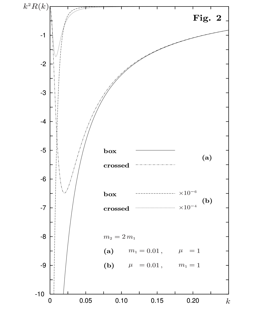
Figure 2: The $k$-dependence of the box and crossed residues are plotted for particular values of $m_{\mbox{\tiny$1$},\mbox{\tiny$2$}}$ and $\mu$. The case (a) and (b) correspond respectively to the exchange of high and small mass scalars.

contribute to the invariant scattering amplitude only for value of $k\ll m_{\mbox{\tiny$1$},\mbox{\tiny$2$}}$. The $k$-dependence of these functions is explicitly shown, for particular values of $m_{\mbox{\tiny$1$},\mbox{\tiny$2$}}$ and $\mu$ in the case (b) of Fig. 2. In this small $\mu$ limit,

$$\frac{R_{\mbox{\tiny$1$}}^{\square}(k)}{R_{\mbox{\tiny$2$}}^{\square}(k)}=-\,\frac{E_{\mbox{\tiny$2$}}-m_{\mbox{\tiny$2$}}}{E_{\mbox{\tiny$1$}}+m_{\mbox{\tiny$1$}}}\,\frac{E_{\mbox{\tiny$2$}}}{E_{\mbox{\tiny$1$}}}\,\left[\,\frac{\mu^{\mbox{\tiny$2$}}+2\,m_{\mbox{\tiny$2$}}\left(E_{\mbox{\tiny$2$}}-m_{\mbox{\tiny$2$}}\right)}{\mu^{\mbox{\tiny$2$}}-2\,m_{\mbox{\tiny$1$}}\left(E_{\mbox{\tiny$1$}}+m_{\mbox{\tiny$1$}}\right)}\,\right]^{\mbox{\tiny$2$}}\approx-\,\frac{k^{\mbox{\tiny$2$}}}{4\,m_{\mbox{\tiny$1$}}^{\mbox{\tiny$2$}}}\,\left(\,\frac{k^{\mbox{\tiny$2$}}+\mu^{\mbox{\tiny$2$}}}{k^{\mbox{\tiny$2$}}+4\,m_{\mbox{\tiny$1$}}^{\mbox{\tiny$2$}}-\mu^{\mbox{\tiny$2$}}}\,\right)^{\mbox{\tiny$2$}}\,\,.$$

This is a very small ratio, so $R_{\mbox{\tiny$2$}}^{\square}(k)$ dominates. This residue can be approximated by

$$k^{\mbox{\tiny$2$}}\,R_{\mbox{\tiny$2$}}^{\square}(k)=-\,(E_{\mbox{\tiny$2$}}+m_{\mbox{\tiny$2$}})\,/\,\left\{\,4\,W\,E_{\mbox{\tiny$2$}}\,\left[\,\mu^{\mbox{\tiny$2$}}+2\,m_{\mbox{\tiny$2$}}\left(E_{\mbox{\tiny$2$}}-m_{\mbox{\tiny$2$}}\right)\right]^{\mbox{\tiny$2$}}\right\}\approx-\,1\,/\,\left[\,2\,W\,\left(k^{\mbox{\tiny$2$}}+\mu^{\mbox{\tiny$2$}}\right)^{\mbox{\tiny$2$}}\,\right]\,\,,$$

and, by making use of the elementary integrals

$$\alpha^{\mbox{\tiny$3$}}\,\int_{\mbox{\tiny$0$}}^{\infty}\frac{\mbox{d}k}{(k^{\mbox{\tiny$2$}}+\alpha^{\mbox{\tiny$2$}})^{{}^{\mbox{\tiny$2$}}}}=\alpha\,\int_{\mbox{\tiny$0$}}^{\infty}\frac{k^{\mbox{\tiny$2$}}\,\mbox{d}k}{(k^{\mbox{\tiny$2$}}+\alpha^{\mbox{\tiny$2$}})^{{}^{\mbox{\tiny$2$}}}}=\frac{\pi}{4}\,\,,$$

we find that

$$\int_{\mbox{\tiny$0$}}^{\infty}\mbox{d}k\,\,k^{\mbox{\tiny$2$}}\,R_{\mbox{\tiny$2$}}^{\square}(k)\approx-\,\frac{\pi}{8\,W\,\mu^{\mbox{\tiny$3$}}}\,\,,$$ (16)

which, as anticipated, is much larger than the contribution of $R_{\mbox{\tiny$1$}}^{\square}(k)$ given by

$$\int_{\mbox{\tiny$0$}}^{\infty}\mbox{d}k\,\,k^{\mbox{\tiny$2$}}\,R_{\mbox{\tiny$1$}}^{\square}(k)\approx\frac{\pi}{64\,W\,m_{\mbox{\tiny$1$}}^{\mbox{\tiny$3$}}}\,\,.$$ (17)

The corresponding crossed contributions are

$$k^{\mbox{\tiny$2$}}\,R_{\mbox{\tiny$1$}}^{\times}(k) = \left(E_{\mbox{\tiny$1$}}+m_{\mbox{\tiny$1$}}\right)\,/\,\left\{\,4\,\Delta\,E_{\mbox{\tiny$1$}}\left[\,\mu^{\mbox{\tiny$2$}}+2\,m_{\mbox{\tiny$1$}}\left(E_{\mbox{\tiny$1$}}-m_{\mbox{\tiny$1$}}\right)\right]^{\mbox{\tiny$2$}}\right\}$$

$$\approx 1\,/\,\left[\,2\,\Delta\,\left(k^{\mbox{\tiny$2$}}+\mu^{\mbox{\tiny$2$}}\right)^{\mbox{\tiny$2$}}\,\right]+k^{\mbox{\tiny$2$}}\,/\,\left[\,8\,m_{\mbox{\tiny$1$}}^{\mbox{\tiny$2$}}\,\Delta\,\left(k^{\mbox{\tiny$2$}}+\mu^{\mbox{\tiny$2$}}\right)^{\mbox{\tiny$2$}}\,\right]\,\,,$$

$$k^{\mbox{\tiny$2$}}\,R_{\mbox{\tiny$2$}}^{\times}(k) = -\,\left(E_{\mbox{\tiny$2$}}+m_{\mbox{\tiny$2$}}\right)\,/\,\left\{\,4\,\Delta\,E_{\mbox{\tiny$2$}}\,\left[\,\mu^{\mbox{\tiny$2$}}+2\,m_{\mbox{\tiny$2$}}\left(E_{\mbox{\tiny$2$}}-m_{\mbox{\tiny$2$}}\right)\right]^{\mbox{\tiny$2$}}\right\}$$

$$\approx -\,1\,/\,\left[\,2\,\Delta\,\left(\,k^{\mbox{\tiny$2$}}+\mu^{\mbox{\tiny$2$}}\right)^{\mbox{\tiny$2$}}\,\right]-k^{\mbox{\tiny$2$}}\,/\,\left[\,8\,m_{\mbox{\tiny$2$}}^{\mbox{\tiny$2$}}\,\Delta\,\left(k^{\mbox{\tiny$2$}}+\mu^{\mbox{\tiny$2$}}\right)^{\mbox{\tiny$2$}}\,\right]\,\,.$$

In these expressions for the crossed residues we have kept higher order terms because the leading contributions cancel. In fact,

$$k^{\mbox{\tiny$2$}}\,\left[\,R_{\mbox{\tiny$1$}}^{\times}(k)+R_{\mbox{\tiny$2$}}^{\times}(k)\,\right]\approx\frac{W}{8\,m_{\mbox{\tiny$1$}}^{\mbox{\tiny$2$}}\,m_{\mbox{\tiny$2$}}^{\mbox{\tiny$2$}}}\,\frac{k^{\mbox{\tiny$2$}}}{\left(k^{\mbox{\tiny$2$}}+\mu^{\mbox{\tiny$2$}}\right)^{\mbox{\tiny$2$}}}\,\,.$$

and hence

$$\int_{\mbox{\tiny$0$}}^{\infty}\mbox{d}k\,\,k^{\mbox{\tiny$2$}}\,\left[\,R_{\mbox{\tiny$1$}}^{\times}(k)+R_{\mbox{\tiny$2$}}^{\times}(k)\,\right]\approx\frac{\pi}{32\,W\,m^{\mbox{\tiny$2$}}\,\mu}\,\,,$$ (18)

where $m=m_{\mbox{\tiny$1$}}m_{\mbox{\tiny$2$}}/W$ is, as before, the reduced mass.

Let us now consider the ”double pole” contributions. Since both $k^{\mbox{\tiny$2$}}$ and $\mu^{\mbox{\tiny$2$}}$ are very small compared to $m_{\mbox{\tiny$1$},\mbox{\tiny$2$}}^{\mbox{\tiny$2$}}$, we can approximate the expressions for $A$, $A_{\times}$ and $B$ by

$$A/m_{\mbox{\tiny$1$}}\approx-\,A_{\times}/m_{\mbox{\tiny$1$}}\approx-\,B/m_{\mbox{\tiny$2$}}\approx C=2\,E_{\mbox{\tiny$0$}}\,\,,$$

whence

$$R_{\mbox{\tiny$0$}}^{\square}(k)\approx-\,R_{\mbox{\tiny$0$}}^{\times}(k)\approx 3\,k^{\mbox{\tiny$2$}}\,/\,\left[\,16\,m_{\mbox{\tiny$1$}}m_{\mbox{\tiny$2$}}\,\left(\,\mu^{\mbox{\tiny$2$}}+k^{\mbox{\tiny$2$}}\right)^{{}^{\mbox{\tiny$5$}/\mbox{\tiny$2$}}}\,\right]\,\,.$$

Now with the help of the elementary integral

$$\alpha^{\mbox{\tiny$2$}}\,\int_{\mbox{\tiny$0$}}^{\infty}\frac{k^{\mbox{\tiny$2$}}\,\mbox{d}k}{(k^{\mbox{\tiny$2$}}+\alpha^{\mbox{\tiny$2$}})^{{}^{\mbox{\tiny$5$}/\mbox{\tiny$2$}}}}=\frac{1}{3}\,\,,$$

we find that

$$\int_{\mbox{\tiny$0$}}^{\infty}\mbox{d}k\,\,k^{\mbox{\tiny$2$}}\,R_{\mbox{\tiny$0$}}^{\square}(k)\approx-\,\int_{\mbox{\tiny$0$}}^{\infty}\mbox{d}k\,\,k^{\mbox{\tiny$2$}}\,R_{\times}^{\square}(k)\approx\frac{1}{16\,W\,m\,\mu^{\mbox{\tiny$2$}}}\,\,.$$ (19)

Finally, the contributions to the scattering amplitude, coming from the fourth order ladder and crossed ladder diagrams, can be analytically expressed by using the leading contributions coming from the single pole $2$ and the double pole $0$ for the box diagram, i.e.

$$\mathcal{M}^{\square}\approx\frac{\lambda_{\mbox{\tiny$1$}}^{{}^{\mbox{\tiny$2$}}}\lambda_{\mbox{\tiny$2$}}^{{}^{\mbox{\tiny$2$}}}}{2\,\pi^{\mbox{\tiny$2$}}}\,\left[\,-\,\frac{\pi}{8\,W\,\mu^{\mbox{\tiny$3$}}}+\,\frac{1}{16\,W\,m\,\mu^{\mbox{\tiny$2$}}}\right]\,\,,$$ (20)

and from the double pole $0$ for the crossed one, i.e.

$$\mathcal{M}^{\times}\approx\frac{\lambda_{\mbox{\tiny$1$}}^{{}^{\mbox{\tiny$2$}}}\lambda_{\mbox{\tiny$2$}}^{{}^{\mbox{\tiny$2$}}}}{2\,\pi^{\mbox{\tiny$2$}}}\,\left[\,-\,\frac{1}{16\,W\,m\,\mu^{\mbox{\tiny$2$}}}\right]\,\,.$$ (21)

These analytic expressions are in excellent agreement with numerical (test) calculations, made for a selected choice of masses. These numerical results have been obtained by using directly Eq.(13), i.e. without any approximations. This is shown in the upper part of Table 1, that for $\mu\ll m_{\mbox{\tiny$1$},\mbox{\tiny$2$}}$, in which by ”analytic box” and ”analytic crossed” we intend the expressions in the brackets of Eqs.(20) and (21).

Comparing now the fourth-order total scattering amplitude,

$$\mathcal{M}^{\square}+\mathcal{M}^{\times}\approx-\,\frac{\lambda_{\mbox{\tiny$1$}}^{{}^{\mbox{\tiny$2$}}}\lambda_{\mbox{\tiny$2$}}^{{}^{\mbox{\tiny$2$}}}}{16\,\pi}\,\frac{1}{W\,\mu^{\mbox{\tiny$3$}}}\,\,,$$ (22)

with the one boson exchange amplitude (7), we find that the fourth-order amplitude is greater or comparable to the second-order amplitude when

$$\frac{\lambda_{\mbox{\tiny$1$}}\lambda_{\mbox{\tiny$2$}}}{16\,\pi\,W\,\mu}\geq 1\,\,.$$ (23)

By using the effective dimensionless coupling strength for the $\Phi^{\mbox{\tiny$3$}}$ Yukawa interaction, see Eq.(6), the previous condition becomes

$$\frac{g_{\mbox{\tiny eff}}^{{}^{\mbox{\tiny$2$}}}}{4\pi}\geq\frac{\mu}{m}\,\,,$$ (24)

which reproduces exactly the Hulthen inequality given in section I.

The fourth order terms considered modify significantly the ”effective” potential in the calculation. As shown by Gross[4] the added potential to the tree diagram Yukawa is given by

$$V_{\mbox{\tiny$2$}\mu}(r)=\frac{1}{8\,\pi}\,\left(\,\frac{g^{\mbox{\tiny$2$}}_{\mbox{\tiny eff}}}{4\,\pi}\,\right)^{\mbox{\tiny$2$}}\,\int_{\mbox{\tiny$2$}\mu}^{\infty}\,\frac{\mbox{d}z}{\sqrt{z^{\mbox{\tiny$2$}}-4\,\mu^{\mbox{\tiny$2$}}}}\,\frac{\exp[-\,z\,r]}{r}\,\,.$$

This represents an integral over higher mass ($>2\mu$) exchanges. It implies a significant addition to the Yukawa. Higher order terms will also produce modifications. We expect that the basic (underlying) Yukawa should become insignificant as we approach the bound state inequality, after which the perturbation series diverges. If the Yukawa is indeed ”smothered” out, it is somewhat surprising that the above bound state inequality is exactly the same as that given by the non-relativistic Hulthen.

Finally, there is an important point, made by Gross[17], that we wish to recall about this approach. The perturbation series (ladder diagrams) considered are relativistically invariant. For small $\mu$ the loop momentum is also small, on average, and consequently the relativistic corrections are small. These corrections are associated principally with the double pole contributions. However, for this particular model, the double pole contributions of the box and crossed diagrams cancel to leading order (see the above approximate equations). This observation will be relevant for our conclusions.

IV. THE EXCHANGE OF HIGH MASS SCALARS

We now proceed to the original part of this work. We consider the case of large $\mu$ exchange, i.e. when $\mu\gg m_{\mbox{\tiny$1$},\mbox{\tiny$2$}}$. We cannot use the approximations used in the previous section, based on small loop momenta and which conveniently approximated the square root terms by polynomials. In this case the average loop momenta exceeds even $\mu$. Furthermore, if one considers the full residues given in section II, one notes that they contain poles for real positive $k$. The $R_{\mbox{\tiny$1$}}^{\square}(k)$ residue has a pole for

$$\mu^{\mbox{\tiny$2$}}-2\,m_{\mbox{\tiny$1$}}\left(E_{\mbox{\tiny$1$}}+m_{\mbox{\tiny$1$}}\right)=0.$$

While the $R_{\mbox{\tiny$0$}}^{\square}(k)$ residue has one when

$$A=0\,\,\,\Rightarrow\,\,\,2\,E_{\mbox{\tiny$0$}}m_{\mbox{\tiny$1$}}=\mu^{\mbox{\tiny$2$}}.$$

We shall now argue that these pole contributions cancel. First we observe, the non-obvious fact, that these singularities occur at the same value of $k$, i.e. at

$$k_{s}=\mu\,\sqrt{\left(\frac{\mu}{2\,m_{\mbox{\tiny$1$}}}\right)^{\mbox{\tiny$2$}}-1}\,\,\gg\mu.$$

This equation confirms their absence for the case considered in the previous section, since the value of $k$ at the pole becomes complex for small $\mu$. On the other hand, there are no pole contributions in the crossed residues. The cancellation of the box poles can be shown both analytically and numerically. We will not give here the analytic proof derived from a Maclaurin series expansion of the box terms about $k_{s}$.

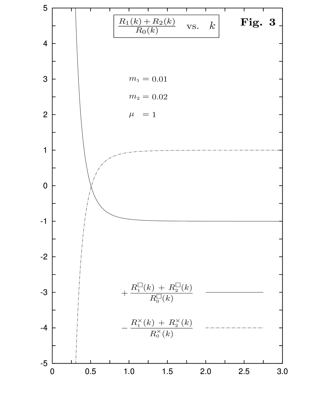
Figure 3: The plots refer to the ratio of $R_{\mbox{\tiny$1$}}(k)$ plus $R_{\mbox{\tiny$2$}}(k)$ over $R_{\mbox{\tiny$0$}}(k)$ for the box and crossed terms. For clarity the crossed terms are plotted with a change of sign. The curves are essentially identical and for $k\geq\mu$ the sum of the three residues cancel.

The numerical argument is essentially based upon Fig. 3. In this figure (drawn for an arbitrary choice of masses compatible with our limit) we plot the ratio

$$\frac{R_{\mbox{\tiny$1$}}(k)+R_{\mbox{\tiny$2$}}(k)}{R_{\mbox{\tiny$0$}}(k)}$$

separately for the box and crossed terms with a change of sign for the crossed terms for clarity of the figure. The region plotted in $k$ includes the pole value $k_{s}$. The curves are essentially identical. The pole terms in the numerator and denominator of the box ratio have cancelled resulting in a smooth curve. Indeed these plots show that there is no observable difference in the sum of the box and of the crossed residues. Furthermore, for $k>0.5\,\mu$ the ratio tends rapidly to one or minus one as the case may be. This means that the the sum of the three residues cancel not only any pole contributions, but cancel ”tout-court” for $k\geq\mu$. This occurs separately for both the box and crossed sums and consequently for the total sum. Another conclusion based upon Fig. 3 is that for $k\ll\mu$,

$$R_{\mbox{\tiny$1$}}(k)+R_{\mbox{\tiny$2$}}(k)\gg R_{\mbox{\tiny$0$}}(k)$$

separately both for the box and crossed terms. Numerical trials have lead us to conclude that integrating $R_{\mbox{\tiny$1$}}(k)+R_{\mbox{\tiny$2$}}(k)$ in $k$ up to $\mu/2$ yields an excellent approximation to the full integration over all three terms. This is useful, not so much for the numerical calculations as for the derivation of a closed expression for the box and crossed diagram contributions. In Table 1 (lower half) we list the numerical and analytic results based upon the above heuristic rule. The agreement is very impressive. The analytic formulas we used for this table are given below and were derived as follows. First note that the poles at $k_{s}$ lie outside our truncated integrated region ($k<\mu/2$) so that the integrals can be performed using elementary formulas. We start with the following simplified expressions for these residues, in which we have dropped, where possible, the incoming scalar masses compared to $\mu$,

$$k^{\mbox{\tiny$2$}}\,R_{\mbox{\tiny$1$}}^{\square}(k) \approx \left(E_{\mbox{\tiny$1$}}-m_{\mbox{\tiny$1$}}\right)\,/\,\left[\,4\,W\,E_{\mbox{\tiny$1$}}\,\mu^{\mbox{\tiny$4$}}\,\right]\,\,,$$

$$k^{\mbox{\tiny$2$}}\,R_{\mbox{\tiny$2$}}^{\square}(k) \approx -\,\left(E_{\mbox{\tiny$2$}}+m_{\mbox{\tiny$2$}}\right)\,/\,\left[\,4\,W\,E_{\mbox{\tiny$2$}}\,\mu^{\mbox{\tiny$4$}}\,\right]\,\,,$$

$$k^{\mbox{\tiny$2$}}\,R_{\mbox{\tiny$1$}}^{\times}(k) \approx \left(E_{\mbox{\tiny$1$}}+m_{\mbox{\tiny$1$}}\right)\,/\,\left[\,4\,W\,E_{\mbox{\tiny$1$}}\,\mu^{\mbox{\tiny$4$}}\,\right]\,\,,$$

$$k^{\mbox{\tiny$2$}}\,R_{\mbox{\tiny$2$}}^{\times}(k) \approx -\,\left(E_{\mbox{\tiny$2$}}+m_{\mbox{\tiny$2$}}\right)\,/\,\left[\,4\,W\,E_{\mbox{\tiny$2$}}\,\mu^{\mbox{\tiny$4$}}\,\right]\,\,.$$

Consequently,

$$k^{\mbox{\tiny$2$}}\,\left[\,R_{\mbox{\tiny$1$}}^{\square}(k)+R_{\mbox{\tiny$2$}}^{\square}(k)\,\right] \approx -\,\frac{1}{4\,W\,\mu^{\mbox{\tiny$4$}}}\,\left(\,\frac{m_{\mbox{\tiny$1$}}}{E_{\mbox{\tiny$1$}}}+\frac{m_{\mbox{\tiny$2$}}}{E_{\mbox{\tiny$2$}}}\,\right)\,\,,$$

$$k^{\mbox{\tiny$2$}}\,\left[\,R_{\mbox{\tiny$1$}}^{\times}(k)+R_{\mbox{\tiny$2$}}^{\times}(k)\,\right] \approx -\,\frac{1}{4\,\Delta\,\mu^{\mbox{\tiny$4$}}}\,\left(\,\frac{m_{\mbox{\tiny$2$}}}{E_{\mbox{\tiny$2$}}}-\frac{m_{\mbox{\tiny$1$}}}{E_{\mbox{\tiny$1$}}}\,\right)\,\,.$$

The integrals up to $\mu/2$ yield,

$$\int_{\mbox{\tiny$0$}}^{\mu/2}\mbox{d}k\,\,k^{\mbox{\tiny$2$}}\,\left[\,R_{\mbox{\tiny$1$}}^{\square}(k)+R_{\mbox{\tiny$2$}}^{\square}(k)\,\right] \approx -\,\frac{1}{4\,W\,\mu^{\mbox{\tiny$3$}}}\,\left(\,\frac{m_{\mbox{\tiny$1$}}}{\mu}\,\,\mbox{arcsinh}\frac{\mu}{2\,m_{\mbox{\tiny$1$}}}+\frac{m_{\mbox{\tiny$2$}}}{\mu}\,\,\mbox{arcsinh}\frac{\mu}{2\,m_{\mbox{\tiny$2$}}}\,\right)\,\,,$$

$$\int_{\mbox{\tiny$0$}}^{\mu/2}\mbox{d}k\,\,k^{\mbox{\tiny$2$}}\,\left[\,R_{\mbox{\tiny$1$}}^{\times}(k)+R_{\mbox{\tiny$2$}}^{\times}(k)\,\right] \approx \,-\,\frac{1}{4\,\Delta\,\mu^{\mbox{\tiny$3$}}}\,\left(\,\frac{m_{\mbox{\tiny$2$}}}{\mu}\,\,\mbox{arcsinh}\frac{\mu}{2\,m_{\mbox{\tiny$2$}}}-\frac{m_{\mbox{\tiny$1$}}}{\mu}\,\,\mbox{arcsinh}\frac{\mu}{2\,m_{\mbox{\tiny$1$}}}\,\right)\,\,.$$

Finally,

$$\mathcal{M}^{\square}\approx\frac{\lambda_{\mbox{\tiny$1$}}^{{}^{\mbox{\tiny$2$}}}\lambda_{\mbox{\tiny$2$}}^{{}^{\mbox{\tiny$2$}}}}{2\,\pi^{\mbox{\tiny$2$}}}\,\left[\,-\,\frac{1}{4\,W\,\mu^{\mbox{\tiny$3$}}}\,\left(\,\frac{m_{\mbox{\tiny$1$}}}{\mu}\,\,\mbox{arcsinh}\frac{\mu}{2\,m_{\mbox{\tiny$1$}}}+\frac{m_{\mbox{\tiny$2$}}}{\mu}\,\,\mbox{arcsinh}\frac{\mu}{2\,m_{\mbox{\tiny$2$}}}\,\right)\right]$$ (25)

and

$$\mathcal{M}^{\times}\approx\frac{\lambda_{\mbox{\tiny$1$}}^{{}^{\mbox{\tiny$2$}}}\lambda_{\mbox{\tiny$2$}}^{{}^{\mbox{\tiny$2$}}}}{2\,\pi^{\mbox{\tiny$2$}}}\,\left[\,-\,\frac{1}{4\,\Delta\,\mu^{\mbox{\tiny$3$}}}\,\left(\,\frac{m_{\mbox{\tiny$2$}}}{\mu}\,\,\mbox{arcsinh}\frac{\mu}{2\,m_{\mbox{\tiny$2$}}}-\frac{m_{\mbox{\tiny$1$}}}{\mu}\,\,\mbox{arcsinh}\frac{\mu}{2\,m_{\mbox{\tiny$1$}}}\,\right)\right]\,\,.$$ (26)

In the lower half of Table 1 (high mass exchange) by ”analytic box” and ”analytic crossed”, we intend the expressions in the brackets of Eqs.(25) and (26). The numerical calculations have been made for the sum of all the three residues and without an explicit cut-off in $k$.

For a more compact expression, we now add these ”analytic” results after approximating the $\mbox{arcsinh}(x/2)$ by $\ln x$, since all our $x$ are very large. After some algebra, we obtain the following formula for the fourth order contributions to the invariant amplitude,

$$\mathcal{M}^{\square}+\mathcal{M}^{\times} \approx \frac{\lambda_{\mbox{\tiny$1$}}^{{}^{\mbox{\tiny$2$}}}\lambda_{\mbox{\tiny$2$}}^{{}^{\mbox{\tiny$2$}}}}{2\,\pi^{\mbox{\tiny$2$}}}\,\left[\,-\,\frac{1}{4\,\mu^{\mbox{\tiny$4$}}}\,\left(\,\ln\frac{\mu^{\mbox{\tiny$2$}}}{m_{\mbox{\tiny$1$}}m_{\mbox{\tiny$2$}}}+\frac{1+\rho^{\mbox{\tiny$2$}}}{1-\rho^{\mbox{\tiny$2$}}}\ln\rho\,\right)\,\right]$$ (27)

$$= -\,\frac{\lambda_{\mbox{\tiny$1$}}^{{}^{\mbox{\tiny$2$}}}\lambda_{\mbox{\tiny$2$}}^{{}^{\mbox{\tiny$2$}}}}{8\,\pi^{{}^{\mbox{\tiny$2$}}}}\,\frac{1}{\mu^{\mbox{\tiny$4$}}}\,\left(\,\ln\frac{\mu^{\mbox{\tiny$2$}}}{m_{\mbox{\tiny$1$}}m_{\mbox{\tiny$2$}}}+\frac{1+\rho^{\mbox{\tiny$2$}}}{1-\rho^{\mbox{\tiny$2$}}}\ln\rho\,\right)\,\,,$$

with $\rho=m_{\mbox{\tiny$1$}}/m_{\mbox{\tiny$2$}}$. As an aside we note that this result is symmetric in the incoming masses $m_{\mbox{\tiny$1$}}$ and $m_{\mbox{\tiny$2$}}$. This natural result is not obvious in the expressions for the fourth order diagrams. The condition for the existence for a bound state in the high mass exchange case thus becomes

$$\frac{g^{\mbox{\tiny$2$}}_{\mbox{\tiny eff}}}{2\,\pi^{{}^{\mbox{\tiny$2$}}}}\geq\frac{\mu^{\mbox{\tiny$2$}}}{m_{\mbox{\tiny$1$}}m_{\mbox{\tiny$2$}}}\,\mbox{\large/}\,\left(\,\ln\frac{\mu^{\mbox{\tiny$2$}}}{m_{\mbox{\tiny$1$}}m_{\mbox{\tiny$2$}}}+\frac{1+\rho^{\mbox{\tiny$2$}}}{1-\rho^{\mbox{\tiny$2$}}}\ln\rho\,\right)\,\,.$$ (28)

This inequality is even simpler when $m_{\mbox{\tiny$1$}}\ll m_{\mbox{\tiny$2$}}$. In this case one obtains

$$\left(\,\ln\frac{\mu^{\mbox{\tiny$2$}}}{m_{\mbox{\tiny$1$}}m_{\mbox{\tiny$2$}}}+\frac{1+\rho^{\mbox{\tiny$2$}}}{1-\rho^{\mbox{\tiny$2$}}}\ln\rho\,\right)\to\,2\ln\frac{\mu}{m_{\mbox{\tiny$2$}}}\,\,,$$

and hence for a bound state to exist (when $m_{\mbox{\tiny$1$}}\ll m_{\mbox{\tiny$2$}}\ll\mu$) one must have

$$g_{\mbox{\tiny eff}}^{\mbox{\tiny$2$}}\geq\pi^{\mbox{\tiny$2$}}\,\displaystyle{\frac{\mu}{m_{\mbox{\tiny$1$}}}\,\frac{\mu/m_{\mbox{\tiny$2$}}}{\ln[\mu/m_{\mbox{\tiny$2$}}]}}\,\,.$$ (29)

Since $\mu/m_{\mbox{\tiny$2$}}\gg\ln[\mu/m_{\mbox{\tiny$2$}}]$, this is an even stronger condition on the coupling strength than the low mass exchange condition, extrapolated to high mass exchange,

$$g_{\mbox{\tiny eff}}^{\mbox{\tiny$2$}}\geq 4\,\pi\,\displaystyle{\frac{\mu}{m_{\mbox{\tiny$1$}}}}\,\,.$$ (30)

We conclude that, in our toy model, bound states for high mass exchanges do not exist unless the effective coupling constant becomes even stronger than that required by the Hulthen condition.

V CONCLUSIONS

We have presented in this paper a calculation of the forward scattering contributions of the fourth order box and lader diagrams for a particular scalar field model. From these results the condition upon the effective coupling strength for the existence of a bound state has been obtained. The requirement imposed was that the sum of these fourth order terms equal or exceed the tree diagram contribution. For small exchanged mass ($\mu\ll m_{\mbox{\tiny$1$},\mbox{\tiny$2$}}$) we have reobtained the result of Franz Gross[4, 17]. In the opposite limit of high exchanged mass ($\mu\gg m_{\mbox{\tiny$1$},\mbox{\tiny$2$}}$) we have derived an inequality for a bound state, albeit as an approximate result. It agrees very well with our numerical integral results for appropriate (but otherwise casually chosen) sets of selected mass values.

A first observation to be made is that the two inequalities, for low and high $\mu/m$, are not the same. One should therefore not extrapolate either outside of their respective domains. In this particular model, the conclusion is that, as the exchanged mass increases, the effective coupling constant must grow even faster than $\sqrt{\mu/m}$ for a bound state to exist. This is a toy model so we have no explicit (physical) limitations, but of course large coupling constants negate the very perturbation series upon which the method is based. However, this is not what we expect to happen for interacting spinors. It is perhaps useful to recall here, more explicitly, some of the arguments upon which our expectations for spinors are based. Amongst the lowest order relativistic corrections to the Schroedinger equation is that which gives rise to the renowned Darwin term [3],

$$\frac{e}{8m^{\mbox{\tiny$2$}}}\,\nabla^{{}^{\mbox{\tiny$2$}}}\,A_{\mbox{\tiny$0$}}(r)\,\,.$$

This term simply adds onto the potential term $eA_{\mbox{\tiny$0$}}(r)$. When the electrostatic potential is a Coulomb potential produced by an opposite charged point (massive) source, we obtain

$$\frac{e^{\mbox{\tiny$2$}}}{8m^{\mbox{\tiny$2$}}}\,\delta^{3}(\boldsymbol{r})\,\,.$$

This contributes only to the $s$ -wave but it is essential for the transformation of the relativistic correction of the Hydrogen energy spectrum into one which depends only upon $j$ (the total angular momentum) in addition to $n$ (the principle quantum number). A result which is automatic in the Dirac equation. We note that since the Darwin term is essential to the s-wave spinor bound states, these are technically ”relativistic” under our definition (see the Introduction). However, when this same term is calculated for a Yukawa potential, we observe that

$$\nabla^{{}^{\mbox{\tiny$2$}}}\,\frac{\exp[-\,\mu\,r]}{r}=\mu^{\mbox{\tiny$2$}}\,\frac{\exp[-\,\mu\,r]}{r}-4\,\pi\,\delta^{3}(\boldsymbol{r})\,\,.$$

The first of these terms augments the Yukawa potential and amplifies the effective coupling constant,

$$g_{\mbox{\tiny eff}}^{\mbox{\tiny$2$}}\to g_{\mbox{\tiny eff}}^{\mbox{\tiny$2$}}\,\left(1+\frac{\mu^{\mbox{\tiny$2$}}}{8m^{\mbox{\tiny$2$}}}\right)\,\,.$$

For $\mu\gg m$,

$$g_{\mbox{\tiny eff}}^{\mbox{\tiny$2$}}\to g_{\mbox{\tiny eff}}^{\mbox{\tiny$2$}}\,\frac{\mu^{\mbox{\tiny$2$}}}{8m^{\mbox{\tiny$2$}}}\,\,,$$

and this is just just what is needed to ”invert” the inequality condition for a bound state from

$$g_{\mbox{\tiny eff}}^{2}>\frac{\mu}{m}\,\,\,\to\,\,\,g_{\mbox{\tiny eff}}^{\mbox{\tiny$2$}}>\frac{8m}{\mu}\,\,.$$

The latter inequality is a weak constraint, easily satisfied, since $m\ll\mu$. Of course, this argument is flawed by the fact that limiting oneself to the lowest order relativistic corrections assumes that they must be small, or at least that the higher order corrections can for some reason (such as cancellations) be totally ignored. Nevertheless, this result does suggest that relativistic effects could be very important for the bound state inequality. In the specific model treated in this paper Gross has shown that the relativistic corrections for small $\mu/m$ come from the poles in the double pole contributions[4]. Now the box and crossed contributions for these double poles cancel in this model. It is therefore a very different situation from the case of interacting spinors. Furthermore, the Klein-Gordon equation does not have a Darwin type term, so Yukawa coupling amplification has not been shown to occur for interacting scalars. On the contrary, the results of this paper demonstrate specifically that it does not occur. It is our intention to consider a more interesting model with incoming spinors exchanging bosons in a future study.

A possible alternative approach in determining the inequality condition for a bound state is to first derive a corresponding two body differential equation (Bethe-Salpeter in this casa of scalar interactions) from which not only the existence of a bound state may be derived but indeed the full bound state spectrum. However, our procedure is the only one available for cases in which the two-body equation is unknown[4].

$m_{\mbox{\tiny$1$}}$	$m_{\mbox{\tiny$2$}}$	$\mu$	$\begin{array}[]{ll}\mbox{Analytic}\\ \mbox{Box}\\ \\ \left[\,\lambda_{\mbox{\tiny$1$}}^{\mbox{\tiny$2$}}\lambda_{\mbox{\tiny$2$}}^{\mbox{\tiny$2$}}\,/\,2\,\pi\,\right]\end{array}$	$\begin{array}[]{ll}\mbox{Numerical}\\ \mbox{Box}\\ \\ \left[\,\lambda_{\mbox{\tiny$1$}}^{\mbox{\tiny$2$}}\lambda_{\mbox{\tiny$2$}}^{\mbox{\tiny$2$}}\,/\,2\,\pi\,\right]\end{array}$	$\begin{array}[]{ll}\mbox{Analytic}\\ \mbox{Crossed}\\ \\ \left[\,\lambda_{\mbox{\tiny$1$}}^{\mbox{\tiny$2$}}\lambda_{\mbox{\tiny$2$}}^{\mbox{\tiny$2$}}\,/\,2\,\pi^{\mbox{\tiny$2$}}\,\right]\end{array}$	$\begin{array}[]{ll}\mbox{Numerical}\\ \mbox{Crossed}\\ \\ \left[\,\lambda_{\mbox{\tiny$1$}}^{\mbox{\tiny$2$}}\lambda_{\mbox{\tiny$2$}}^{\mbox{\tiny$2$}}\,/\,2\,\pi^{\mbox{\tiny$2$}}\,\right]\end{array}$
$1$	$2$	$10^{-\mbox{\tiny$3$}}$	$-\,1.3087\times 10^{\mbox{\tiny$8$}}$	$-\,1.3087\times 10^{\mbox{\tiny$8$}}$	$-\,3.1250\times 10^{\mbox{\tiny$4$}}$	$-\,3.1232\times 10^{\mbox{\tiny$4$}}$
$1$	$4$	$10^{-\mbox{\tiny$3$}}$	$-\,7.8524\times 10^{\mbox{\tiny$7$}}$	$-\,7.8524\times 10^{\mbox{\tiny$7$}}$	$-\,1.5625\times 10^{\mbox{\tiny$4$}}$	$-\,1.5617\times 10^{\mbox{\tiny$4$}}$
$2$	$4$	$10^{-\mbox{\tiny$3$}}$	$-\,6.5442\times 10^{\mbox{\tiny$7$}}$	$-\,6.5442\times 10^{\mbox{\tiny$7$}}$	$-\,7.8125\times 10^{\mbox{\tiny$3$}}$	$-\,7.8104\times 10^{\mbox{\tiny$3$}}$
$1$	$2$	$10^{-\mbox{\tiny$2$}}$	$-\,1.3059\times 10^{\mbox{\tiny$5$}}$	$-\,1.3059\times 10^{\mbox{\tiny$5$}}$	$-\,3.1250\times 10^{\mbox{\tiny$2$}}$	$-\,3.1067\times 10^{\mbox{\tiny$2$}}$
$10^{-\mbox{\tiny$2$}}$	$2\times 10^{-\mbox{\tiny$2$}}$	$1$	$-\,1.0358$	$-\,1.0363$	$-\,0.8049$	$-\,0.8059$
$10^{-\mbox{\tiny$2$}}$	$4\times 10^{-\mbox{\tiny$2$}}$	$10$	$-\,1.4497\times 10^{-\mbox{\tiny$4$}}$	$-\,1.4497\times 10^{-\mbox{\tiny$4$}}$	$-\,1.2648\times 10^{-\mbox{\tiny$4$}}$	$-\,1.2649\times 10^{-\mbox{\tiny$4$}}$
$2\times 10^{-\mbox{\tiny$2$}}$	$4\times 10^{-\mbox{\tiny$2$}}$	$10$	$-\,1.4381\times 10^{-\mbox{\tiny$4$}}$	$-\,1.4382\times 10^{-\mbox{\tiny$4$}}$	$-\,1.2071\times 10^{-\mbox{\tiny$4$}}$	$-\,1.2071\times 10^{-\mbox{\tiny$4$}}$
$10^{-\mbox{\tiny$2$}}$	$2\times 10^{-\mbox{\tiny$2$}}$	$10$	$-\,1.6114\times 10^{-\mbox{\tiny$4$}}$	$-\,1.6114\times 10^{-\mbox{\tiny$4$}}$	$-\,1.3804\times 10^{-\mbox{\tiny$4$}}$	$-\,1.3804\times 10^{-\mbox{\tiny$4$}}$

Table 1: We list the numerical and analytic results for the exchange of small (upper half) and high (lower half) mass scalars. The analytic formulas for the small $\mu$ limit refer for the box diagram to the expression in the brackets of Eq.(20) and for the crossed one to that of Eq.(21). The analytic formulas for the high $\mu$ limit refer to Eqs. (25) and (26).

References

• [1] C. Cohen-Tannoudji, B. Diu and F. LaloΓ«, Quantum mechanics, John Wiley & Sons, Paris (1977).
• [2] C. Itzykson and J.B. Zuber, Quantum field theory, McGraw-Hill, Singapore (1985).
• [3] J. J. Sakurai, Advanced quantum mechanics, Addison-Wesley, New York (1987).
• [4] F. Gross, Relativistic quantum mechanics and field theory, John & Wiley Sons, New York (1993).
• [5] S. De Leo and P. Rotelli, ”Amplification of coupling for Yukawa potentials”, Phys. Rev. D 69, 034006-5 (2004).
• [6] O. Klein, ”Die reflexion von elektronrn an einem potentialsprun nach der relativistichen dynamik von Dirac”, Z. Phys. 53, 157-165 (1929).
• [7] A. Hansen and F. Ravndal, ”Klein paradox and its resolution”, Phys. Scr. 23, 1036-1402 (1981).
• [8] M. Soffel, B. MΓΌller, and W. Greiner, ”Stability and decay of the Dirac vacuum in external gauge fields”, Phys. Rep. 85, 51-122 (1982).
• [9] P. Krekora, Q. Su, and R. Grobe, ”Klein paradox in spatial and temporal resolution”, Phys. Rev. Lett. 92, 040406-4 (2004).
• [10] S. De Leo and P. Rotelli, ”Barrier paradox in the Klein zone”, Phys. Rev. A 73, 042107-7 (2005).
• [11] S. FlΓΌgge, Practical quantum mechanics, Springer-Verlag, Berlin (1999).
• [12] W. E. Lamb and R. C. Retherford, ”Fine structure of the hydrogen atom by a microwave method ”, Phys. Rev. 72, 241-243 (1947).
• [13] H. A. Bethe and E. E. Salpeter, ”A relativistic equation for bound-state problems ”, Phys. Rev. 84, 1232-1242 (1951).
• [14] E. E. Salpeter, ”Mass corrections to the fine structure of hydrogen-like atoms ”, Phys. Rev. 87, 328-343 (1952).
• [15] H. A. Bethe and E. E. Salpeter, Quantum mechanics of one and two electron atoms, Springer-Verlag, Berlin (1957).
• [16] R. Blankenbecher and R. Sugar, ”Linear integral equations for relativistic multichannel scattering”, Phys. Rev. 142, 1051-1059 (1966).
• [17] F. Gross, ”Three-dimensional covariant integral equations for low-energy systems”, Phys. Rev. 186, 1448-1462 (1969)
• [18] B. Kayser, ”Neutrino mass, mixing and flavor change”, J. Phys. G 33, 156-164 (2006).