0020308/RI

D-branes at multicritical points

Matthias R. Gaberdiel^♣, Dan Israël^♠ and Eliezer Rabinovici^⋄

$\clubsuit$ Institut für Theoretische Physik, eth Zürich, 8093 Zürich, Switzerland

^♠ greco, Institut d’Astrophysique de Paris, 98bis Bd Arago, 75014 Paris, France

^⋄ Racah Institute of Physics, The Hebrew University, Jerusalem 91904, Israel

Abstract

The moduli space of $c=1$ conformal field theories in two dimensions has a multicritical point, where a circle theory is equivalent to an orbifold theory. We analyse all the conformal branes in both descriptions of this theory, and find convincing evidence that the full brane spectrum coincides. This shows that the equivalence of the two descriptions at this multicritical point extends to the boundary sector. We also perform the analogous analysis for one of the multicritical points of the ${\cal N}=1$ superconformal field theories at $c=\tfrac{3}{2}$. Again the brane spectra are identical for both descriptions, however the identification is more subtle.

1 Introduction

Moduli spaces of two-dimensional conformal field theories (cfts) often contain multicritical points, where different lines (or hypersurfaces) of theories, generated by a set of marginal operators, intersect. These points are quite interesting as they admit several equivalent, but superficially different, descriptions. More precisely, each formulation of the multicritical point has the same set of primary fields (w.r.t. the chiral algebra of the model), whose operator product expansions are given by the same structure constants. However, the different formulations typically have different spacetime interpretations. For example, for the case of the bosonic cft at $c=1$, the circle theory at twice the self-dual radius is equivalent to the $\mathbb{Z}_{2}$ orbifold of the self-dual circle theory [1, 2].

A natural question that arises in this context is whether these seemingly different descriptions of the same bulk cft admit the same set of boundary conditions and boundary operators when defined on surfaces with boundaries, i.e. the same D-branes and open string sectors in the string theory language. As the D-branes are non-perturbative objects in space-time, they can be thought of as refined probes compared to fundamental strings [3]. They could therefore uncover unexpected distinctions between the different descriptions of the multicritical points.

One approach to the construction of D-branes is in terms of boundary states that lie in a suitable completion of the closed string spectrum. These states are certain linear combinations of the Ishibashi states [4] that have to satisfy a number of consistency conditions [5, 6]. This construction can be performed purely in terms of the closed string theory, and thus will be the same for the different descriptions of a given multicritical point. However, a priori, it is not guaranteed that only one set of consistent boundary states exists for a given closed string theory, and thus the different descriptions of a multicritical point may have different D-brane spectra. Indeed, each description of the multicritical point has a specific space-time interpretation, and thus comes with a certain set of ‘canonical’ D-branes: for example, the circle theory is described by an action and it implies that the theory must have Dirichlet and Neumann branes (since these can be defined in terms of the action); similarly, the orbifold of the circle theory contains always the orbifold invariant combinations of the branes of the circle theory, etc. Since the various D-branes of a theory must be mutually consistent (and since one can determine the open string moduli from the open string spectra), these ‘canonical’ D-branes typically determine the full D-brane spectrum of the bulk theory uniquely. It is then an interesting question to ask whether these D-brane spectra agree for the different descriptions of a multicritical point.

The multicritical points are also special since they have additional marginal operators (relative to the marginal operators that exist at a generic point on each line) that allow one to move along the other branch. According to the general analysis of boundary deformations [8] one may then expect that there is a similar enhancement of the brane moduli space. However, in general the analysis is more complicated since the brane moduli space may also be bigger than what one would expect from the (preserved) symmetries of the bulk theory [9].

In this paper we shall analyse the complete D-brane spectra for the different descriptions of various multicritical points. We shall concentrate on those cases where we have full control of the bulk and brane moduli spaces of the different theories. Besides the minimal models (that do not admit marginal deformations) the only examples known so far are free theories of bosons and fermions with central charge and (local) superconformal symmetry $(c=1$, ${\cal N}=0)$, $(c=\tfrac{3}{2}$, ${\cal N}=1)$ and $(c=3$, ${\cal N}=2)$ [10, 11, 12, 13]. The first two cases are more interesting, as both the bulk and brane moduli spaces are quite rich. In both cases, the bulk moduli space has multicritical points (one for ${\cal N}=0$ and five for ${\cal N}=1$), and the brane moduli space has components that are described by discrete quotients of SU(2), that exists only for particular discrete values of the compactification radius. It was found in [10, 11, 12] that, on top of the usual Dirichlet and Neumann branes, this accounts for a complete set of boundary states. (For certain radii, the Dirichlet or Neumann branes may be part of the continuous component. Note also that these boundary conditions all define unitary open string spectra; more general non-unitary boundary conditions are parametrised by elements in SL(2,$\mathbb{C}$).)

In this paper we work out the complete dictionary between the full brane moduli spaces in the $(c=1$, ${\cal N}=0)$ model at the multicritical point, where the circle and the orbifold lines intersect [2]. In the $(c=\tfrac{3}{2}$, ${\cal N}=1)$ theory, all but one multicritical point have rather uninteresting brane moduli spaces as they do not contain many superconformal boundary states beyond the usual Dirichlet and Neumann branes. We will therefore focus on the multicritical point, where the circle theory and the super-orbifold theory become equivalent [14]. For both multicritical points we shall find that the D-brane spectra of the two descriptions agree; in the superconformal case however a number of intricate subtleties arise that we explain in detail.

The plan of the paper is as follows. Section 2 is devoted to the analysis of the $c=1$ models, with a review of the necessary material. In section 3 we consider the $\hat{c}=1$ ($c=\tfrac{3}{2}$) theories. Finally, section 4 contains our conclusions.

2 The c=1 multicritical point

The moduli space of $c=1$ conformal field theories is well known [2]. First of all there is the family of models corresponding to a free real boson $X(z,\bar{z})$ at radius $R$, the circle line. This model has a U(1) symmetry that is enhanced to an $\hat{\rm su}(2)_{1}\times\hat{\rm su}(2)_{1}$ affine algebra at the self-dual radius $R=\tfrac{1}{\sqrt{2}}$. Secondly, the moduli space contains a line of theories that are obtained by the $\mathbb{Z}_{2}$ orbifold $\mathcal{I}~{}:X\mapsto-X$ from the circle theory; this family of theories is usually called the orbifold line. Finally, the moduli space contains isolated points obtained by orbifolding the circle theory at the self-dual radius by the tetrahedral, octohedral and icosahedral discrete subgroups of SU(2). They play no role in our discussion. (Branes for these theories have been constructed in [15].)

The circle and orbifold lines intersect for $R_{\rm circ}=\sqrt{2}$ and $R_{\rm orb}=\tfrac{1}{\sqrt{2}}$. In fact, the circle theory at twice the self-dual radius is also an orbifold (that is sometimes denoted by SU(2)/$\mathcal{C}_{2}$), and it is not difficult to show that it is in fact equivalent to the above $\mathbb{Z}_{2}$ orbifold (that is sometimes denoted by SU(2)/$\mathcal{D}_{1}$) [2].

2.1 Boundary states of the circle line: a reminder

We first review the construction of the boundary states on the circle line following [10, 11, 12]. For a generic radius $R$, the brane moduli space is rather simple: it consists of standard Dirichlet and Neumann branes that preserve the U(1) chiral symmetry of the model, each parametrised by a U(1) moduli (the position of the brane and the Wilson line, respectively). In addition there is a continuous family of branes that only couple to the vacuum representation of the U(1) theory.

For radii of the form $R=\tfrac{M}{N\sqrt{2}}$, with $M$ and $N$ coprime, the situation is more interesting [11]: in addition to the Neumann and Dirichlet branes there are additional conformal branes preserving only the Virasoro algebra that are parametrised by elements in SU$(2)/\mathbb{Z}_{M}\times\mathbb{Z}_{N}$. Their origin can be understood from two different points of view. First, one can think of the theory at radius $R=\tfrac{M}{N\sqrt{2}}$ as a $\mathbb{Z}_{M}\times\mathbb{Z}_{N}$ orbifold of the self-dual circle theory, where $\mathbb{Z}_{M}$ ($\mathbb{Z}_{N}$) acts via momentum (winding) shifts [16]. By taking orbifold invariant combinations, the conformal branes of the self-dual circle theory (that are parametrised by SU(2)) then lead to the above moduli space of conformal branes.

Secondly, we can classify all conformal Ishibashi states, and then construct the corresponding boundary states from them as in [11]. To explain this in more detail we note that if the radius of the circle is $R=\tfrac{M}{N\sqrt{2}}$, some of the $\hat{\rm u}(1)$ representations decompose into infinitely many Virasoro representations. This happens whenever the conformal weight of a U(1) primary is of the form $\Delta=r^{2}$, $r\in\mathbb{N}/2$ (i.e. when the U(1) representation has charge $q=\sqrt{2}r$), and the complete decomposition into Virasoro irreducible representations is of the form

$$\mathcal{V}^{\mathfrak{u}_{1}}_{\sqrt{2}r}=\bigoplus_{\ell=0}^{\infty}\mathcal{V}^{\mathfrak{Vir}}_{(r+\ell)^{2}}\ .$$ (2.1)

According to Cardy’s analysis [6] to each of these representations one can associate an Ishibashi state that is a solution of the gluing condition $T(z)=\bar{T}(\bar{z})$ on the real axis. In this way one obtains Virasoro Ishibashi states $|j,m,\bar{m}\rangle\hskip-2.56073pt\rangle$, where the quantum number $j\in\mathbb{N}/2$ denotes the irreducible Virasoro representation of conformal weight $\Delta=j^{2}$, while $m$, $\bar{m}$ (with $j-m$ and $j-\bar{m}$ integer, $|m|,|\bar{m}|\leqslant j$) parametrise the $\hat{\rm u}(1)_{\rm L}\times\hat{\rm u}(1)_{\rm R}$ representations in which this Virasoro Ishibashi state appears [8, 17, 11]. Depending on the specific choice of the radius, there are certain selection rules which the $m$ and $\bar{m}$ have to satisfy.

Let us now specialise the discussion to the case $(M=2,N=1)$, the multicritical point. From the point of view of the circle line it corresponds to a compactification at radius $R=\sqrt{2}$, i.e. twice the self-dual radius. It is obtained as a $\mathbb{Z}_{2}$ winding shift orbifold of the self-dual point, $\tilde{X}\sim\tilde{X}+\pi/\sqrt{2}$. The left and right conformal weights of the $\hat{\rm u}(1)\times\hat{\rm u}(1)$ primaries read

$$\Delta=\left(\frac{n}{4}+w\right)^{2}\equiv m^{2}\ ,\qquad\bar{\Delta}=\left(\frac{n}{4}-w\right)^{2}\equiv\bar{m}^{2}\ ,$$ (2.2)

where $n$ ($w$) denotes the momentum (winding) number. Note that the theory possesses a pair of marginal operators with $(n=0,w=\pm 1)$; a certain linear combination of these states is the marginal operator that allows one to move along the orbifold line.

Let us discuss the boundary states of this theory. As for any radius, there are standard Dirichlet and Neumann branes. The Dirichlet branes involve the Dirichlet Ishibashi states $|(n,0)\rangle\hskip-2.56073pt\rangle$ built on momentum primaries with quantum numbers $(n,0)$ , while the Neumann Ishibashi states $|(0,w)\rangle\hskip-2.56073pt\rangle$ arise in the winding sectors $(0,w)$. In addition we have the Virasoro Ishibashi states $|j,m,\bar{m}\rangle\hskip-2.56073pt\rangle$ that come from the degenerate $\hat{\rm u}(1)$ representations. At $R=\sqrt{2}$, the relevant constraint on $m$ and $\bar{m}$ is simply

$$m-\bar{m}\equiv 0\mod 2\ .$$ (2.3)

We can think of this constraint as coming from an orbifold action, as the circle theory at $R=\sqrt{2}$ is the $\mathcal{C}_{2}$ orbifold of the self-dual circle theory. In terms of the SU(2) description, the orbifold acts as $g\mapsto\sigma_{3}g\sigma_{3}\equiv{\rm Ad}_{\sigma_{3}}g$. Thus the conformal branes of the circle theory at $R=\sqrt{2}$ are of the form [11]

$$|\!|g\rangle\hskip-2.56073pt\rangle_{\rm circ}=2^{1/4}\sum_{j,m,\bar{m}}\frac{1}{2}\Bigl{[}D^{j}_{m,\bar{m}}(g)+D^{j}_{m,\bar{m}}\left({\rm Ad}_{\sigma_{3}}\,g\right)\Bigr{]}|j,m,\bar{m}\rangle\hskip-2.56073pt\rangle\ ,$$ (2.4)

where $D^{j}_{m,\bar{m}}(g)$ is the SU(2) matrix element of $g$ in the $j$-representation. Obviously $g$ and ${\rm Ad}_{\sigma_{3}}\,g$ describe the same boundary state, and thus the moduli space of these branes is SU(2)$/\mathbb{Z}_{2}$.

For off-diagonal group elements, i.e. group elements of the form $g=i\sigma_{1}e^{i\sigma_{3}\phi}$, the resulting brane is in fact a usual Neumann brane with Wilson line $\tilde{x}_{0}=\phi/\sqrt{2}$ (that only involves the Ishibashi states $|(0,w)\rangle\hskip-2.56073pt\rangle$). On the other hand, for diagonal group elements $g=e^{i\sigma_{3}\theta}$ with $\theta\in[0,2\pi)$, the above brane is not fundamental, but rather describes the superposition of two Dirichlet branes at opposite points on the circle. One way to see this is to note that the condition on $m$ and $\bar{m}$ in (2.2) to be half-integer implies that only Ishibashi states with even $n$ appear in the boundary state (2.4) — the superposition of two Dirichlet branes at opposite points on the circle projects out the odd momentum states and only couples to even momentum states, see for example (2.5) below. The fact that these branes are not fundamental is also natural from a standard orbifold point of view. The branes (2.4) are the usual regular branes of the orbifold SU(2)/$\mathcal{C}_{2}$. As in other examples [18] such branes can be resolved into fractional branes whenever they sit on a fixed point of the orbifold. Since the group action is $g\mapsto{\rm Ad}_{\sigma_{3}}\,g$, the fixed point set consists just of the diagonal SU(2) matrices. If $g$ is diagonal, the corresponding brane can be resolved into a pair of fundamental Dirichlet branes, whose boundary states include both even and odd momentum Ishibashi states

$$|\!|D;\theta\rangle\hskip-2.56073pt\rangle=2^{-\nicefrac{{3}}{{4}}}\sum_{n\in\mathbb{Z}}e^{i\frac{n\theta}{2}}|(n,0)\rangle\hskip-2.56073pt\rangle\ .$$ (2.5)

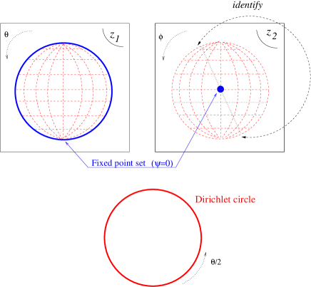
Figure 1: Two sections of the brane moduli space of the circle theory, with the Dirichlet circle added. Antipodal points in the $z_{2}$-plane are identified.

To summarise, the single brane moduli space is made of the quotient SU(2)/$\mathcal{C}_{2}$ with the circle $g=e^{i\sigma_{3}\theta}$ removed, together with a disconnected $U(1)$ component that describes the single Dirichlet brane moduli space. It is convenient to parametrise the SU(2) group elements in terms of Euler angles

$$g=e^{\frac{i\sigma_{3}}{2}(\theta+\phi)}e^{i\sigma_{1}\psi}e^{\frac{i\sigma_{3}}{2}(\theta-\phi)}\ .$$ (2.6)

Then the $\mathcal{C}_{2}$ orbifold acts as $\phi\mapsto\phi+\pi$. The fixed point set of this orbifold is $\psi=0$, i.e. the circle spanned by $\theta\in[0,2\pi)$. Using the embedding of the three-sphere in $\mathbb{C}^{2}$

$$z_{1}=\cos\psi\,e^{i\theta}\ ,\qquad z_{2}=\sin\psi\,e^{i\phi}\ ,$$ (2.7)

one gets the representation of the moduli space of fig. 1. The fixed point set of the orbifold should be removed from the one-brane moduli space. Instead one has a separate component of the moduli space, isomorphic to $U(1)$, describing a single Dirichlet brane sitting on the circle at $x=\theta/\sqrt{2}$ with $\theta\in[0,4\pi)$.

Finally, it is interesting to notice that the Dirichlet branes are not sensitive to the underlying $SU(2)$ symmetry of the theory, as their moduli space describes a disconnected $U(1)$ component of the full brane moduli space.

Comments on D-brane moduli space and target space geometry

One may ask whether there is any interesting relation between the moduli space of D-branes, and the target space geometry. In particular, one may expect that the moduli space of the D0-brane describes a ‘quantum version’ of the target space geometry. However, an immediate problem with this idea is that it is a priori not clear how to characterise the D0-branes (among all conformal branes, say). Typically, the full moduli space of conformal branes may contain different connected components, and one may wonder whether all of them lead to the same geometric interpretation, or whether different brane probes may see ‘different geometries’.

For example, in standard torus compactifications, the brane moduli space contains (typically) different connected components corresponding to different Dp-branes. These different components of the moduli space lead in general to different geometries. However, the resulting geometries are all related by T-duality to one another (and so describe equivalent string backgrounds); this is simply a consequence of the fact that every Dp-brane can be transformed, by a suitable T-duality transformation, to a D0-brane. Thus, in this case, every such component of the brane moduli space can be thought of as a D0-brane moduli space, and hence leads to a geometric interpretation in the above sense. The different geometries one obtains in this way describe the different ‘geometrical interpretations’ one may give to the string theory in question. All of them describe, however, equivalent conformal field theories.

For the circle theory we have been considering so far, the full D-brane moduli space is under control, and one may test this idea further. For a generic radius, the full brane moduli space contains three connected components: the connected part of the moduli space of the Virasoro or conformal branes — this excludes the Neumann and Dirichlet branes unless they are already part of it (which only happens is the radius is a multiple or a fraction of the self-dual radius); the moduli space of Dirichlet branes, and the moduli space of Neumann branes. In each case we should then consider the sigma model whose target space is the brane moduli space in question. In order to define such a sigma model one obviously needs to have a metric on the brane moduli space; this can be naturally obtained from the open string correlation functions. It is a priori not obvious whether the resulting sigma-model is conformal; to make it conformal will sometimes require that certain $B$-fields are also switched on. For this to work the open string marginal operator correlation functions in the appropriate sector should encode a $B$-field, just as they encode a metric. Such a $B$-field is, for example, required for the case of the moduli space of the conformal branes which (for a ‘rational’ radius) is the quotient $SU(2)/\mathbb{Z}_{M}\times\mathbb{Z}_{N}$; with the $B$-field the resulting conformal sigma-model is then the $\mathbb{Z}_{M}\times\mathbb{Z}_{N}$ orbifold of the $SU(2)$ wzw model at level $k=1$. So the ‘geometry’ that is associated to these branes is $SU(2)/\mathbb{Z}_{M}\times\mathbb{Z}_{N}$.

The analysis for the Neumann or Dirichlet moduli spaces is simpler: both are equivalent to a circle, which describes, on the nose, a conformal sigma-model. The only difference is that the radius of the circle we obtain in this manner is different for the Dirichlet and Neumann branes. However, the two radii are related to one another by T-duality (as in the case of the Dp-branes mentioned above), and thus the resulting geometries are equivalent in string theory.

For the case at hand, the three brane moduli space components lead to a circle (for the case of the Neumann and Dirichlet branes), and $SU(2)/\mathbb{Z}_{M}\times\mathbb{Z}_{N}$ (for the case of the conformal branes). Superficially, the latter geometry is rather different from a circle; however, as a conformal field theory, it is precisely equivalent to it again: the circle theory at radius $R=(M/N)R_{\rm sd}$ is a $\mathbb{Z}_{M}\times\mathbb{Z}_{N}$ orbifold of the self-dual radius theory, which in turn is equivalent to the level $k=1$ $SU(2)$ wzw model! So even in this more complicated example, it seems that the different components of the brane moduli space lead to equivalent quantum geometries. It would be very interesting to analyse whether this observation generalises to other backgrounds as well.

2.2 Boundary states of the orbifold

The orbifold acts on the circle theory by the involution $\mathcal{I}~{}:Y(z,\bar{z})\mapsto-Y(z,\bar{z})$, where in order to avoid confusion with the circle description we now denote the boson by $Y$. The closed string spectrum consists of the invariant states of the circle theory; in addition we have two twisted sectors that are built on the two twist fields $\sigma^{y_{0}}(z,\bar{z})$ (associated with the two fixed points at $y_{0}=0,\pi R$). These twist fields have conformal dimension $\Delta=\bar{\Delta}=1/16$, and the oscillators are half-integer moded in the twisted sector.

Let us now specialise to the self dual radius $R=1/\sqrt{2}$. As at any radius we have the usual Dirichlet branes that are obtained by symmetrising the circle Dirichlet branes under the orbifold action

$$|\!|D;y\rangle\hskip-2.56073pt\rangle_{\rm orb}=2^{1/4}\sum_{n\in\mathbb{Z}}\cos(\sqrt{2}ny)\,|(n,0)\rangle\hskip-2.56073pt\rangle\ ,$$ (2.8)

where $y\in(0,\pi/\sqrt{2})$. These branes are fundamental, except if they sit at one of the two fixed points $y_{0}=0,\pi/\sqrt{2}$. If this is the case, one can resolve them into fractional Dirichlet branes that also involve the twisted sector Ishibashi states (where $y_{0}=0,\pi/\sqrt{2}$)

$$|D;y_{0}\rangle\hskip-2.56073pt\rangle_{\rm tw}=e^{\sum_{r=1/2}^{\infty}\frac{1}{r}b_{-r}\bar{b}_{-r}}\ \sigma^{y_{0}}|0\rangle\ .$$ (2.9)

The resulting fractional branes are then [19]

$$|\!|D,y_{0};\pm\rangle\hskip-2.56073pt\rangle_{\rm orb}=\tfrac{1}{2}\,|\!|D;y_{0}\rangle\hskip-2.56073pt\rangle_{\rm orb}\pm 2^{-\nicefrac{{1}}{{4}}}|D;y_{0}\rangle\hskip-2.56073pt\rangle_{\rm tw}\ ,$$ (2.10)

where $y_{0}=0,\pi/\sqrt{2}$. The situation is similar for the Neumann branes. The orbifold invariant combination of the Neumann branes are

$$|\!|N;\tilde{y}\rangle\hskip-2.56073pt\rangle_{\rm orb}=2^{1/4}\sum_{w\in\mathbb{Z}}\cos(\sqrt{2}w\tilde{y})\,|(0,w)\rangle\hskip-2.56073pt\rangle\ .$$ (2.11)

The appropriate combination of Neumann Ishibashi states from the twisted sector reads

$$|N;\tilde{y}_{0}\rangle\hskip-2.56073pt\rangle_{\rm tw}=\frac{1}{\sqrt{2}}\,e^{-\sum_{r=1/2}^{\infty}\frac{1}{r}b_{-r}\bar{b}_{-r}}\ \left[\sigma^{0}+e^{i\sqrt{2}\tilde{y}_{0}}\,\sigma^{\frac{\pi}{\sqrt{2}}}\right]|0\rangle\ ,$$ (2.12)

where $\tilde{y}_{0}=0,\tfrac{\pi}{\sqrt{2}}$. As for the Dirichlet branes, the full Neumann fractional brane boundary states are then

$$|\!|N,\tilde{y}_{0};\pm\rangle\hskip-2.56073pt\rangle=\tfrac{1}{2}\,|\!|N;\tilde{y}_{0}\rangle\hskip-2.56073pt\rangle_{\rm orb}\pm 2^{-\nicefrac{{1}}{{4}}}|N;\tilde{y}_{0}\rangle\hskip-2.56073pt\rangle_{\rm tw}\ .$$ (2.13)

These are the well-known standard constructions, but one can also obtain the additional conformal boundary states for this theory. Indeed, the orbifold can be thought of as the SU(2) orbifold by $\mathcal{D}_{1}$.

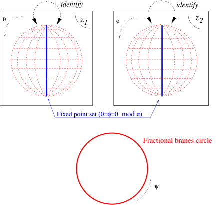
Figure 2: Two sections of the brane moduli space of the orbifold theory, with the fractional branes circle added.

This orbifold acts on SU(2) group elements as $g\mapsto\sigma_{1}g\sigma_{1}$. Indeed, the operator $\mathcal{I}$ acts on $\hat{\rm u}(1)\times\hat{\rm u}(1)$ primaries as $(m,\bar{m})\mapsto(-m,-\bar{m})$, and hence maps the Virasoro Ishibashi states as

$$|j,m,\bar{m}\rangle\hskip-2.56073pt\rangle\mapsto|j,-m,-\bar{m}\rangle\hskip-2.56073pt\rangle\ .$$ (2.14)

This is then reproduced by $g\mapsto\sigma_{1}g\sigma_{1}$ since (see (A.2) for the definition of these matrix elements)

$$D^{j}_{-m-\bar{m}}(g)=(-)^{m-\bar{m}}D^{j}_{m\bar{m}}(g^{\star})=D^{j}_{m\bar{m}}(\sigma_{3}g^{\star}\sigma_{3})=D^{j}_{m\bar{m}}(\sigma_{1}g\sigma_{1})\ .$$ (2.15)

Thus the orbifold invariant boundary states are simply

$$|\!|g\rangle\hskip-2.56073pt\rangle_{\rm orb}=2^{1/4}\,\sum_{j,m,\bar{m}}\frac{1}{2}\Bigl{[}D^{j}_{m,\bar{m}}\left(g\right)+D^{j}_{m,\bar{m}}\left({\rm Ad}_{\sigma_{1}}\,g\right)\Bigr{]}\,|j,m,\bar{m}\rangle\hskip-2.56073pt\rangle\ .$$ (2.16)

The branes are fundamental unless $g$ belongs to the fixed point set of the orbifold, i.e.  unless $g$ is a matrix of the form $g=e^{i\sigma_{1}\psi}$. It contains the particular cases $\psi=0,\pi$ and $\psi=\pi/2,3\pi/2$. The former corresponds to the Dirichlet brane at the two fixed points, while the latter are the Neumann branes at the T-dual fixed points — see the discussion above. We postpone the construction of the fractional branes for generic $\psi$ to the next subsection. For the moment we only note that, in terms of the Euler angles parametrisation of SU(2), see (2.6), the orbifold acts as $\theta\mapsto-\theta$ and $\phi\mapsto-\phi$, and the fixed point set corresponds to $\theta=\phi=0$. Using the same embedding in $\mathbb{C}^{2}$ one gets the moduli space depicted in fig. 2.

2.3 Mapping of moduli spaces and resolution of the orbifold branes

In the previous subsection we have obtained the full brane moduli space of the circle and the orbifold theories at the multicritical point. For the circle theory, there is a continuous family of conformal branes parametrised by $SU(2)/\mathcal{C}_{2}$, with a circle removed corresponding to the fixed point set of the orbifold. This circle is replaced by a disconnected $S^{1}$ component corresponding to the moduli space of a single Dirichlet brane. For the orbifold theory we also have a continuous family of conformal branes parametrised by $SU(2)/\mathcal{D}_{1}$ (the orbifold is different, although isomorphic), again with a circle removed corresponding to the fixed point set of the orbifold. We expect on general grounds that the corresponding branes can be resolved into two fractional branes; for special points (that correspond either to standard Dirichlet and or Neumann branes) we have already described this above, and we shall construct the resolution for the other branes below. It is interesting to note (as was already observed in [8]) that the family of resolved branes interpolates between fractional Dirichlet and fractional Neumann branes.

Our strategy will be to assume that the two brane moduli spaces are equivalent. We can then use the known resolution of the fixed point branes of the circle theory — these are pairs of Dirichlet branes at opposite points on the circle, that are resolved into single Dirichlet branes — in order to determine what the resolution of the fixed point branes in the orbifold theory should be. As we shall see, the resulting picture satisfies a number of non-trivial consistency conditions, thus suggesting that our identification has been correct.

Relating the generic conformal branes

We start by identifying the generic conformal branes of both theories that are parametrised by SU$(2)/\mathbb{Z}_{2}$. As we have explained above, these branes contain the standard Neumann branes of the circle theory, as well as the standard (non-fixed point) Neumann and Dirichlet branes of the orbifold. The correspondence must relate the two different $\mathbb{Z}_{2}$ actions into one another, and one finds that this is achieved by the rotation matrix of Euler angles $(\psi=\pi/4;\theta=\pi/2;\phi=0)$, i.e. the map

$$\rho~{}:\ g_{\rm circ}\mapsto g_{\rm orb}=\rho(g_{\rm circ})=h\,g_{\rm circ}\,h^{-1}\quad\text{with}\qquad h=\frac{i}{\sqrt{2}}\left(\begin{array}[]{cc}1&1\\ 1&-1\end{array}\right)\ ,$$ (2.17)

which has the property $\rho(\sigma_{3}g\sigma_{3})=\sigma_{1}\rho(g)\sigma_{1}$. Thus we have the dictionary

$$|\!|g\rangle\hskip-2.56073pt\rangle_{\rm circ}\Longleftrightarrow|\!|\rho(g)\rangle\hskip-2.56073pt\rangle_{\rm orb}\ .$$ (2.18)

Under this map, the pairs of antipodal Dirichlet branes in the circle theory (i.e. the group elements $g=e^{i\sigma_{3}\theta}$) are mapped to orbifold branes with

$$g_{\textsc{d}}=\left(\begin{array}[]{cc}\cos\theta&i\sin\theta\\ i\sin\theta&\cos\theta\end{array}\right)\ ,$$ (2.19)

corresponding to the fixed point set of the orbifold. These are neither Dirichlet (diagonal $g$) nor Neumann (off-diagonal $g$) boundary states, except for particular values of $\theta$. For $\theta=\{0;\pi\}$ (the ‘Dirichlet points’) one gets a regular Dirichlet brane sitting at one of the two orbifold fixed points, while for $\theta=\{\tfrac{\pi}{2};\tfrac{3\pi}{2}\}$ (the ‘Neumann points’) one gets a regular Neumann brane at a T-dual fixed point.

As another special case, the Neumann branes of the circle theory are mapped to orbifold branes with

$$g_{\textsc{n}}=\left(\begin{array}[]{cc}i\sin\psi&-\cos\psi\\ \cos\psi&-i\sin\psi\end{array}\right)\ .$$ (2.20)

These are fundamental branes for any $\psi$, as are the corresponding Neumann branes in the circle theory.

Resolution of the orbifold branes

Before we can discuss the dictionary between the fractional branes, we first need to understand the resolution of the fixed point branes in the orbifold theory. We expect on general grounds that the resolved branes will involve Ishibashi states from the twisted sector. We therefore need to understand first what Virasoro Ishibashi states appear in the twisted sector of the orbifold.

The twisted sector $\hat{\rm u}(1)$ representation of the orbifold is not an irreducible Virasoro representation; for example, the state $b_{-1/2}\sigma^{y_{0}}$ is a Virasoro highest weight state. On the other hand, the conformal dimensions that appear ($\Delta=\tfrac{1}{16}+\tfrac{N}{2}$ with $N\in\mathbb{N}$) all correspond to non-degenerate Virasoro representations. Thus one can determine the decomposition based on the comparison of characters. The chiral twisted character of a single fixed point is

$$\sqrt{\frac{\eta(\tau)}{\vartheta_{4}(\tau)}}=\frac{\sqrt{\vartheta_{2}(\tau)\vartheta_{3}(\tau)}}{\sqrt{2}\eta(\tau)}=\frac{\vartheta_{2}(\tau/2)}{2\eta(\tau)}=\sum_{\ell=0}^{\infty}\frac{q^{\frac{1}{4}(\ell+\nicefrac{{1}}{{2}})^{2}}}{\eta(\tau)}\ ,$$ (2.21)

where we have used standard $\vartheta$-function identities, see appendix A. The characters that appear on the right hand side are all characters of irreducible Virasoro representations. By the standard argument we therefore obtain Virasoro Ishibashi states from the twisted sector labelled by

$$|(\ell+\nicefrac{{1}}{{2}})^{2}/4;y_{0}\rangle\hskip-2.56073pt\rangle_{\rm Vir}\ ,$$

where $y_{0}=0,\tfrac{\pi}{\sqrt{2}}$ labels the two fixed points. Note that these Ishibashi states are in one-to-one correspondence with the Dirichlet Ishibashi states $|(n,0)\rangle\hskip-2.56073pt\rangle$ of the circle theory corresponding to odd $n$. (This is in fact guaranteed by the equivalence of the two closed string spectra.) We fix their normalisation by requiring that

$$|D;y_{0}\rangle\hskip-2.56073pt\rangle_{\rm tw}=\sum_{\ell=0}^{\infty}|(\ell+\nicefrac{{1}}{{2}})^{2}/4;y_{0}\rangle\hskip-2.56073pt\rangle_{\rm Vir}\ .$$ (2.22)

For the Neumann twisted sector Ishibashi states, we have to take care of the extra minus sign in the coherent state, see eqn. (2.12). It follows that if the Virasoro highest weight vector involves an odd number of oscillators, the corresponding Ishibashi state appears with a relative minus sign. A Virasoro highest weight vector of conformal weight $\Delta=1/16+\ell(\ell+1)/4$ is made out of an even number of oscillators provided that $\ell(\ell+1)/4\in\mathbb{Z}$, i.e. for $\ell\equiv 0$ or $1\mod 4$. Thus it follows that

$$|N;\tilde{y}_{0}\rangle\hskip-2.56073pt\rangle_{\rm tw}=\frac{1}{\sqrt{2}}\sum_{\ell=0}^{\infty}(-)^{\frac{\ell(\ell+1)}{2}}\left[|(\ell+\nicefrac{{1}}{{2}})^{2}/4;0\rangle\hskip-2.56073pt\rangle_{\rm Vir}+e^{i\sqrt{2}\tilde{y}_{0}}|(\ell+\nicefrac{{1}}{{2}})^{2}/4;\nicefrac{{\pi}}{{\sqrt{2}}}\rangle\hskip-2.56073pt\rangle_{\rm Vir}\right]\ .$$ (2.23)

Because of the symmetries of the problem there is some arbitrariness in the mapping between the (fractional) branes. We choose to identify the pair of Dirichlet branes at $x=\{0;\pi\sqrt{2}\}$ with the unresolved orbifold Dirichlet brane sitting at the fixed point $y=0$, consistently with the map (2.17). It implies that the single Dirichlet brane at $x=0$ is mapped for instance to the Dirichlet fractional brane (2.10) with positive sign; with this convention the single Dirichlet brane at $x=\pi\sqrt{2}$ corresponds then to the fractional Dirichlet brane (2.10) with negative sign. By comparing the boundary state  (2.22) with the odd-momenta coupling of (2.5) it follows that we identify

$$|D;(2\ell+1,0)\rangle\hskip-2.56073pt\rangle+|D;(-2\ell-1,0)\rangle\hskip-2.56073pt\rangle=|(\ell+\nicefrac{{1}}{{2}})^{2}/4;y_{0}=0\rangle\hskip-2.56073pt\rangle_{\rm Vir}\ .$$ (2.24)

The pair of Dirichlet branes at $x=\{\nicefrac{{\pi}}{{\sqrt{2}}};\nicefrac{{3\pi}}{{\sqrt{2}}}\}$ in the circle theory should then be identified with the unresolved orbifold Dirichlet brane sitting at the fixed point $y=\nicefrac{{\pi}}{{\sqrt{2}}}$, using (2.17). This leads to the identification

$$i(-)^{\ell}\Big{[}|D;(2\ell+1,0)\rangle\hskip-2.56073pt\rangle-|D;(-2\ell-1,0)\rangle\hskip-2.56073pt\rangle\Big{]}=|(\ell+\nicefrac{{1}}{{2}})^{2}/4;y_{0}=\nicefrac{{\pi}}{{\sqrt{2}}}\rangle\hskip-2.56073pt\rangle_{\rm Vir}\ .$$ (2.25)

These two linear relations (2.24, 2.25) now fix the dictionary between the twisted sector Ishibashi states of both theories completely. Since we know already how to resolve the fixed point branes of the circle theory (these are just standard single Dirichlet branes) we can now make an ansatz for the resolved branes of the orbifold theory, using these relations. This leads to

$$|\!|e^{i\sigma_{1}\psi};\pm\rangle\hskip-2.56073pt\rangle_{\rm orb} = \tfrac{1}{2}\,|\!|g=e^{i\sigma_{1}\psi}\rangle\hskip-2.56073pt\rangle_{\rm orb}$$

$$\pm\,2^{-\nicefrac{{1}}{{4}}}\sum_{\ell=0}^{\infty}\Bigl{\{}\cos((\ell+\tfrac{1}{2})\psi)\,|(\ell+\nicefrac{{1}}{{2}})^{2}/4;0\rangle\hskip-2.56073pt\rangle_{\rm Vir}$$

$$\qquad\qquad\qquad+(-)^{\ell}\sin((\ell+\tfrac{1}{2})\psi)\,|(\ell+\nicefrac{{1}}{{2}})^{2}/4;\nicefrac{{\pi}}{{\sqrt{2}}}\rangle\hskip-2.56073pt\rangle_{\rm Vir}\Bigr{\}}\ .$$

As a consistency check of this analysis we can now verify that the branes at $\psi=\tfrac{\pi}{2}$ and $\psi=\tfrac{3\pi}{2}$ correspond to the Neumann branes with Wilson lines $\tilde{y}_{0}=0$ and $\tilde{y}_{0}=\tfrac{\pi}{\sqrt{2}}$, respectively. Indeed, we find that, for instance,

$$|\!|e^{i\sigma_{1}\pi/2};\pm\rangle\hskip-2.56073pt\rangle_{\rm orb}=\tfrac{1}{2}\,|\!|e^{i\sigma_{1}\pi/2}\rangle\hskip-2.56073pt\rangle_{\rm orb}\\ \pm\,2^{-\nicefrac{{3}}{{4}}}\sum_{\ell=0}^{\infty}(-)^{\frac{\ell(\ell+1)}{2}}\Bigl{\{}|(\ell+\nicefrac{{1}}{{2}})^{2}/4;0\rangle\hskip-2.56073pt\rangle_{\rm Vir}+|(\ell+\nicefrac{{1}}{{2}})^{2}/4;\nicefrac{{\pi}}{{\sqrt{2}}}\rangle\hskip-2.56073pt\rangle_{\rm Vir}\Bigr{\}}\ ,$$ (2.27)

which is exactly the same expression as the Neumann fractional brane boundary state with Wilson line $\tilde{y}_{0}=0$, see eqn. (2.13) together with (2.23). The analysis for $\psi=3\pi/2$ is essentially identical.

In summary we have thus constructed the resolution of the general conformal fixed point branes of the orbifold theory by assuming that the branes of the circle and the orbifold theory are equivalent. Our ansatz has passed the fairly non-trivial consistency check that it reproduces correctly the known resolution of both Dirichlet and Neumann branes of the orbifold theory. We regard this as convincing evidence that the proposed resolution, as well as the identification of the brane moduli spaces, is indeed correct.

Incidentally, our analysis also implies that all of these resolved branes of the orbifold theory actually preserve a $\hat{\rm u}(1)$ symmetry, not just the Virasoro symmetry (because the corresponding branes of the circle theory do); the relevant chiral currents are $(J,\bar{J})=(\cos 2\sqrt{2}X_{L}(z),\cos 2\sqrt{2}X_{R}(\bar{z}))$. Unfortunately, it is however rather difficult to verify this directly.

3 The ĉ=1 moduli space

Next we want to consider the $\mathcal{N}=(1,1)$ superconformal field theories with $\hat{c}=\tfrac{2c}{3}=1$. As for its bosonic counterpart considered in the previous section, there is a continuous moduli space of such theories, with additional isolated points. All lines of theories can be obtained as orbifolds of the theory of a free boson and a free Majorana fermion. Since there are a number of different orbifolds one may consider (involving in particular the fermion number), the moduli space is quite rich and contains five different lines of theories (circle, orbifold, super-affine, orbifold-prime and super-orbifold), intersecting pairwise at five different multicritical points (we refer the reader to [14] for details). In order to obtain a modular invariant partition function we have to chose a gso-projection; for the circle theory we shall consider the 0B-type gso-projection in the following.

Among the multicritical points, four are such that none of the non-trivial super-$\hat{\rm u}(1)$ representations that appear in the spectrum are reducible with respect to the $\mathcal{N}=1$ super-Virasoro (SVir) algebra; at these multicritical points the brane spectrum will therefore be rather small, and will in particular not contain any component related to SU(2) besides the identity component that is common to all non-rational radii. However, this is not the case for the multicritical point where the circle line at $R=1$ intersects the super-orbifold line also at $R=1$. In that case the spectrum contains many degenerate SVir representations, and hence the brane moduli space is fairly rich. This is not accidental as both theories are (isomorphic) $\mathbb{Z}_{2}$-orbifolds of the super-affine $\hat{\rm so}(3)_{1}\times\hat{\rm so}(3)_{1}$ theory , i.e. the theory of three left- and three right-moving Majorana-Weyl fermions with identical boundary conditions on the torus. Since this is the most interesting case, we shall restrict ourselves to this multicritical point in the following.

We shall be interested in the branes that preserve the $\mathcal{N}=1$ superconformal symmetry, i.e. that satisfy the gluing condition

$$\left(L_{n}-\bar{L}_{-n}\right)|\!|B;\eta\rangle\hskip-2.56073pt\rangle=0\ ,\qquad\left(G_{r}+i\eta\,\bar{G}_{-r}\right)|\!|B;\eta\rangle\hskip-2.56073pt\rangle=0\ ,$$ (3.1)

where $\eta=\pm 1$ labels the two possible superconformal gluing conditions. We will consider the two cases separately as they give rise to different sets of branes and have subtle differences regarding the dictionary of the D-branes.

3.1 Branes of the circle line

We begin with the analysis of the free boson and fermion theory, i.e. the tensor product of the $c=1$ circle line (a free boson at radius $R$) with an Ising model, i.e. a pair of Majorana-Weyl worldsheet fermions $\chi,\,\bar{\chi}$. This is the theory that was studied in [11].

As before, we first have to find all SVir Ishibashi states, i.e. we have to analyse which SVir representations are degenerate. In the Neveu-Schwartz (ns) sector a SVir representation is degenerate if the highest weight has conformal dimension $\Delta=\nicefrac{{r^{2}}}{{2}}$ with $r$ integer. The first null vector is then at level $r+\nicefrac{{1}}{{2}}$, which has therefore the opposite worldsheet fermion number parity compared to the primary state. A super-$\hat{\rm u}(1)$ representation with charge $r$ decomposes then into irreducible SVir representations as

$$\mathcal{V}^{\mathfrak{u}_{1},\,\textsc{ns}}_{r}=\sum_{\ell=0}^{\infty}\mathcal{V}^{\mathfrak{SVir}\,,\,\textsc{ns}}_{(r+\ell)^{2}/2}\ .$$ (3.2)

In this decomposition the SVir representations have (chiral) worldsheet fermion number $F=\ell\mod 2$. In the Ramond (r) sector the SVir representations are degenerate for $\Delta=\nicefrac{{r^{2}}}{{2}}+\nicefrac{{1}}{{16}}$ with $r\in\mathbb{N}+\nicefrac{{1}}{{2}}$ (the null vector is also at level $r+\nicefrac{{1}}{{2}}$). Super $\hat{\rm u}(1)$ primaries with such conformal weights (in the nsns and rr sectors) occur whenever the compactification radius is rational. We consider the case $R=1$ below, relevant for the analysis of the circle/super-orbifold multicritical point. The left and right conformal dimensions of the $\hat{\rm u}(1)$ primaries then read

$$\Delta=\frac{1}{2}\left(\frac{n}{2}+w\right)^{2}+\frac{a^{2}}{16}\equiv\frac{m^{2}}{2}+\frac{a^{2}}{16}\ ,\qquad\bar{\Delta}=\frac{1}{2}\left(\frac{n}{2}-w\right)^{2}+\frac{a^{2}}{16}\equiv\frac{\bar{m}^{2}}{2}+\frac{a^{2}}{16}\ ,$$ (3.3)

where $a=0$ ($a=1$) in the ns (r) sector.

Boundary states in the NSNS sector

Let us start with the nsns sector Ishibashi states. The super-$\hat{u}(1)$ representations are reducible with respect to the SVir algebra if the momentum $n$ is even. From the decomposition of these representations into irreducible SVir $\times$ SVir representations of dimension $\Delta=\bar{\Delta}=\nicefrac{{j^{2}}}{{2}}$, one obtains a set of Ishibashi states $|j,m,\bar{m};\eta\rangle\hskip-2.56073pt\rangle_{\textsc{ns}}$, where $j\in\mathbb{N}$, $j-m$, $j-\bar{m}$ are integer and $|m|,|\bar{m}|\leqslant j$. The label $\eta$ denotes the parameter in the gluing condition (3.1). The superconformal branes in the nsns sector, constructed out of this set of Ishibashi states, then read [11]

$$|\!|g;\eta\rangle\hskip-2.56073pt\rangle_{\textsc{ns}}=\frac{1}{\sqrt{2}}\,\sum_{j\in\mathbb{N},\,m,\bar{m}}\Bigl{[}D^{j}_{m\bar{m}}\left(g\right)+D^{j}_{m\bar{m}}\left({\rm Ad}_{\sigma_{3}}\,g\right)\Bigr{]}\,|j,m,\bar{m};\eta\rangle\hskip-2.56073pt\rangle_{\textsc{ns}}\ .$$ (3.4)

The sum in square brackets imposes the constraint that $m-\bar{m}$ is even (since the winding number $w$ is integer); the constraint that the momentum number $n$ is even is automatically satisfied since $j$ (and hence $m$ and $\bar{m}$) is integer. The boundary state is invariant under the diagonal gso-projection for both choices of $\eta$. Indeed, the SVir $\times$ SVir representation with $\Delta=\bar{\Delta}=j^{2}/2$ is such that $j=m+\ell=\bar{m}+\bar{\ell}$. Since $m-\bar{m}$ is even, so is $\ell-\bar{\ell}$, and it follows from the discussion below eqn (3.2) that all Ishibashi states are gso-invariant.

As before, the boundary state corresponding to $g$ and to ${\rm Ad}_{\sigma_{3}}\,g$ are the same. Furthermore, branes parametrised by $g$ and $-g$ are identical, as $D^{j}_{m\bar{m}}(-g)=(-)^{2j}D^{j}_{m\bar{m}}(g)$. Thus the moduli space of nsns sector boundary states is SO$(3)/\mathbb{Z}_{2}$.

For off-diagonal SU(2) group elements (i.e. group elements of the form $g=i\sigma_{1}e^{i\sigma_{3}\phi}$), one gets an ordinary nsns sector Neumann boundary state, with couplings to all winding states (as $m=-\bar{m}=w$ is not constrained). On the other hand, diagonal group elements ($g=e^{i\sigma_{3}\theta}$) describe a pair of Dirichlet branes since only even momentum states ($n$ even) contribute. The single Dirichlet branes occur as the resolution of these branes; their boundary state is given by

$$|\!|D;x;\eta\rangle\hskip-2.56073pt\rangle_{\textsc{ns}}=\frac{1}{\sqrt{2}}\sum_{n\in\mathbb{Z}}e^{inx}|(n,0)\rangle\hskip-2.56073pt\rangle\otimes|D;\eta\rangle\hskip-2.56073pt\rangle_{\textsc{ns}}\ ,$$ (3.5)

where $|D;\eta\rangle\hskip-2.56073pt\rangle_{\textsc{ns}}$ is the nsns Dirichlet fermion Ishibashi state solving

$$\Bigl{(}\chi_{r}-i\eta\bar{\chi}_{-r}\Bigr{)}|D;\eta\rangle\hskip-2.56073pt\rangle_{\textsc{ns}}=0\ .$$ (3.6)

The parameter $x$ denotes the position of the brane with $x=\theta/2$ and $\theta\in[0,4\pi)$.

Boundary states in the RR sector

In the rr sector the discussion is more subtle because of the fermionic zero modes. First we see from (3.3) that the super-$\hat{\rm u}(1)$ representations are degenerate with respect to the SVir algebra for odd momentum $n$. Analogously to what we have done above, we thus get SVir Ishibashi states $|j,m,\bar{m};\eta\rangle\hskip-2.56073pt\rangle_{\textsc{r}}$ where now $(j,m,\bar{m})$ are half-integer moded. The boundary states then read

$$|\!|g;\eta\rangle\hskip-2.56073pt\rangle_{\textsc{r}}=\frac{1}{\sqrt{2}}\,\sum_{j\in\mathbb{N}+\tfrac{1}{2},\,m,\bar{m}}\Bigl{[}D^{j}_{m\bar{m}}\left(g\right)+D^{j}_{m\bar{m}}\left({\rm Ad}_{\sigma_{3}}\,g\right)\Bigr{]}|j,m,\bar{m};\eta\rangle\hskip-2.56073pt\rangle_{\textsc{r}}\ .$$ (3.7)

As before the boundary states associated to $g$ and ${\rm Ad}_{\sigma_{3}}\,g$ are identical, but now the boundary state corresponding to $g$ and $-g$ have opposite sign. The projection in the square bracket guarantees, as before, that only terms with $m-\bar{m}$ even contribute.

The analysis of the gso-projection is slightly subtle. Using the conventions of [11], the superconformal Ishibashi states satisfy

$$(-)^{F+\bar{F}}|j,m,\bar{m};\eta\rangle\hskip-2.56073pt\rangle_{\textsc{r}}=-\eta(-)^{m-\bar{m}}|j,m,\bar{m};\eta\rangle\hskip-2.56073pt\rangle_{\textsc{r}}\ ,$$ (3.8)

while the fermionic Dirichlet and Neumann Ishibashi states obey

$$(-)^{F+\bar{F}}|D;\eta\rangle\hskip-2.56073pt\rangle_{\textsc{r}}=-\eta\,|D;\eta\rangle\hskip-2.56073pt\rangle_{\textsc{r}}\ ,\qquad(-)^{F+\bar{F}}|N;\eta\rangle\hskip-2.56073pt\rangle_{\textsc{r}}=\eta\,|N;\eta\rangle\hskip-2.56073pt\rangle_{\textsc{r}}\ .$$ (3.9)

Here $|D;\eta\rangle\hskip-2.56073pt\rangle_{\textsc{r}}$ is characterized by the gluing condition (3.6), while the gluing condition for $|N;\eta\rangle\hskip-2.56073pt\rangle_{\textsc{r}}$ has the opposite sign, $(\chi_{r}+i\eta\bar{\chi}_{-r})|N;\eta\rangle\hskip-2.56073pt\rangle=0$. Note that this is consistent with the fact that Dirichlet Ishibashi states appear with $m=\bar{m}$, while for Neumann Ishibashi states we always have $m=-\bar{m}$; in the r-sector $m$ and $\bar{m}$ are half-integer, and hence $m-\bar{m}$ is odd.

As before, the rr-sector boundary states (3.7) are fundamental unless $g$ is diagonal. For diagonal $g$, we have again a pair of Dirichlet branes which can be resolved; the resolved single Dirichlet brane boundary state

$$|\!|D;x;\eta\rangle\hskip-2.56073pt\rangle_{\textsc{r}}=\frac{1}{\sqrt{2}}\sum_{n\in\mathbb{Z}}e^{inx}|(n,0)\rangle\hskip-2.56073pt\rangle\otimes|D;\eta\rangle\hskip-2.56073pt\rangle_{\textsc{r}}$$ (3.10)

then couples to even and odd momenta $n$, whereas (3.7) only involves terms with odd $n$ (since $m$ and $\bar{m}$ are half-integer).

The full boundary states are finally obtained by putting nsns- and rr-sector boundary states together. Their structure depends on the choice of $\eta$ in (3.1). For $\eta=-1$, all SVir Ishibashi states are gso-invariant, and we get

$$|\!|g;\eta=-1\rangle\hskip-2.56073pt\rangle=\frac{1}{\sqrt{2}}\Bigl{(}|\!|g;\eta=-1\rangle\hskip-2.56073pt\rangle_{\textsc{ns}}+i|\!|g;\eta=-1\rangle\hskip-2.56073pt\rangle_{\textsc{r}}\Bigr{)}\ .$$ (3.11)

The brane with $-g$ is the antibrane of that with $g$, but we have the identification that $g$ and ${\rm Ad}_{\sigma_{3}}g$ describe the same D-brane. The moduli space is therefore SU$(2)/\mathbb{Z}_{2}$. These branes are fundamental unless $g$ is diagonal; for diagonal $g$ we can resolve the brane into a Dirichlet brane anti-brane pair sitting at opposite points on the circle. The full boundary state of a single Dirichlet brane is of the form

$$|\!|D;x;-\rangle\hskip-2.56073pt\rangle=\frac{1}{\sqrt{2}}\Bigl{(}|\!|D;x;-\rangle\hskip-2.56073pt\rangle_{\textsc{ns}}+i|\!|D;x;-\rangle\hskip-2.56073pt\rangle_{\textsc{r}}\rangle\Bigr{)}\ .$$ (3.12)

On the other hand, for $g$ off-diagonal, the brane (3.11) describes a Neumann brane that does not involve a rr component — these branes are the analogues of the non-bps branes that were first studied by Sen [21]. This is in agreement with the fact that for $\eta=-1$ the rr-sector Neumann Ishibashi states are gso-odd — see (3.9).

For $\eta=+1$, all rr SVir Ishibashi states $|j,m,\bar{m}\rangle\hskip-2.56073pt\rangle_{\textsc{rr}}$ are gso-odd. Thus for $\eta=+1$ the boundary states $|\!|g;\eta=+1\rangle\hskip-2.56073pt\rangle_{\textsc{ns}}$ are consistent by themselves. As discussed above, the corresponding moduli space is SO$(3)/\mathbb{Z}_{2}$. The branes are fundamental provided that $g$ is neither diagonal nor off-diagonal: the branes with $g$ diagonal describe the superposition of two non-bps Dirichlet branes at opposite points on the circle (that only involve nsns-sector Ishibashi states). For $g$ off-diagonal, on the other hand, the above $\mathbb{Z}_{2}$ (that inverts the signs of the off-diagonal matrix elements of $g$) acts trivially on SO$(3)$ and the branes get resolved into a superposition of a Neumann brane anti-brane pair, i.e. in branes with opposite rr charge. (For $\eta=+1$, the rr-sector Neumann Ishibashi states are gso-invariant.)

3.2 Super-affine line

Although the multicritical point we are interested in lies on the intersection of the circle and the super-orbifold line, it is useful to discuss first the branes of the super-affine line, as it contains the point of maximally extended symmetry in the $\hat{c}=1$ moduli space. Indeed for $R=1$ the super-affine theory is identical to a theory of three Majorana fermions with identical boundary conditions, realising an $\hat{\rm so}(3)_{1}\times\hat{\rm so}(3)_{1}$ Kač-Moody algebra with $\mathcal{N}=(1,1)$ supersymmetry.

The super-affine theory can be obtained from the circle theory as the orbifold by the symmetry $\mathcal{S}\,:\ s_{\textsc{x}}(-)^{F_{st}}$, where $s_{\textsc{x}}$ is the shift symmetry $X\mapsto X+\pi R$ while $F_{st}$ denotes the left-moving spacetime fermion number. Thus $(-)^{F_{st}}$ acts as $+1$ ($-1$) on the nsns (rr) sector. The full torus partition function of the super-affine theory is

$$\mathcal{Z}(\tau)=\frac{1}{2}\sum_{\gamma,\delta\in\mathbb{Z}_{2}}\sum_{n,w\in\mathbb{Z}}(-)^{\delta n}\frac{q^{\frac{1}{8}\left(\frac{n}{R}+R(2w+\gamma)\right)^{2}}}{\eta(\tau)}\frac{\bar{q}^{\frac{1}{8}\left(\frac{n}{R}-R(2w+\gamma)\right)^{2}}}{\bar{\eta}(\bar{\tau})}\frac{1}{2}\sum_{a,b\in\mathbb{Z}_{2}}(-)^{a\delta+b\gamma+\gamma\delta}\left|\frac{\vartheta\left[{a\atop b}\right]}{\eta}\right|.$$ (3.13)

Note that (as is usual for $(-)^{F_{st}}$ orbifolds), the gso-projection is reversed in the twisted sector ($\gamma=1$). Furthermore, the spacetime fermion number parity is opposite in the twisted sector, i.e. it acts as $-1$ in the twisted nsns sector and as $+1$ in the twisted rr sector.

Boundary states of the super-affine theory at R=1

Let us now construct the branes of the super-affine theory at $R=1$, starting from the circle theory at $R=1$. In the untwisted nsns sector, the orbifold by $\mathcal{S}$ has the effect of projecting onto even-momentum states, which implies that all the superconformal Ishibashi states $|j,m,\bar{m};\eta\rangle\hskip-2.56073pt\rangle_{\textsc{ns}}$ are orbifold-invariant (as they all have $n=m+\bar{m}$ even by construction). On the other hand, the additional Dirichlet Ishibashi states with $n$ odd are projected out. Thus all superconformal Ishibashi states in the untwisted sector nsns sector are of the form $|j,m,\bar{m};\eta\rangle\hskip-2.56073pt\rangle_{\textsc{ns}}$ with $j$ integer and $m-\bar{m}$ even.

In the untwisted rr sector, the rr ground states are odd under $(-)^{F_{st}}$, and thus only odd momentum states survive. Again all the superconformal Ishibashi states $|j,m,\bar{m};\eta\rangle\hskip-2.56073pt\rangle_{\textsc{r}}$ are invariant under the orbifold projection (since $n=m+\bar{m}$ is now odd), while the even momentum states in (3.10) are again projected out. The same also applies to the Neumann Ishibashi states (for which $n=0$). Thus all superconformal Ishibashi states in the untwisted rr sector are of the form $|j,m,\bar{m};\eta\rangle\hskip-2.56073pt\rangle_{\textsc{ns}}$ with $j$ half-integer and $m-\bar{m}$ even.

In the $\mathcal{S}$-twisted sector of the super-affine theory, the winding number $w$ is half-integer (see eqn. (3.13) for $\gamma=1$). In the twisted nsns-sector, we therefore get superconformal Ishibashi states labelled by $|j,m,\bar{m};\eta\rangle\hskip-2.56073pt\rangle_{\textsc{ns};\,\rm tw}$, where $j$ is still integer, but now $m-\bar{m}$ is odd. As mentioned above, the ground state of the twisted nsns sector is now gso-odd, and therefore these Ishibashi states survive the gso-projection. They also survive the orbifold projection by $\mathcal{S}$ since $n=m+\bar{m}$ is now odd, but the twisted nsns sector is also odd under $(-)^{F_{st}}$. Taken together with the Ishibashi states of the untwisted nsns sector we therefore have SVir Ishibashi states associated to $(j,m,\bar{m})$, where $j$ is integer, but without any constraints on $m-\bar{m}$.

The analysis for the Ishibashi states from the twisted rr sector is similar. We find superconformal Ishibashi states labelled by $|j,m,\bar{m};\eta\rangle\hskip-2.56073pt\rangle_{\textsc{r};\,\rm tw}$, where $j$ is half-integer, but now $m-\bar{m}$ is odd. Since the GSO-projection in the twisted sector is opposite to what one had before, they are gso-invariant for $\eta=-1$ (and gso-odd for $\eta=+1$). Furthermore they are orbifold invariant since $n=m+\bar{m}$ is now even as is the $(-)^{F_{st}}$ parity of the twisted rr. Together with the superconformal Ishibashi states of the untwisted rr sector we therefore get SVir Ishibashi states associated to $(j,m,\bar{m})$, where $j$ is half-integer, but without any constraints on $m-\bar{m}$. These states are only gso-invariant for $\eta=-1$.

It is now straightforward to construct the boundary states of the super-affine theory. In the nsns the boundary states are simply given by

$$|\!|g\rangle\hskip-2.56073pt\rangle_{\textsc{ns};\,{\rm s-a}}=\sum_{j\in\mathbb{N},m,\bar{m}}D^{j}_{m\bar{m}}\left(g\right)|j,m,\bar{m};\eta\rangle\hskip-2.56073pt\rangle_{\textsc{ns}}\ ,$$ (3.14)

where $j\in\mathbb{N}$, $m,\,\bar{m}\in\mathbb{Z}$ with $|m|,|\bar{m}|<j$, but with no further restrictions on $m,\bar{m}$. In the rr sector we have instead

$$|\!|g\rangle\hskip-2.56073pt\rangle_{\textsc{r};\,{\rm s-a}}=\sum_{j\in\mathbb{N}+\frac{1}{2},m,\bar{m}}D^{j}_{m\bar{m}}\left(g\right)|j,m,\bar{m};\eta\rangle\hskip-2.56073pt\rangle_{\textsc{r}}\ ,$$ (3.15)

where $j,m$ and $\bar{m}$ are now half-integer with $|m|,|\bar{m}|\leqslant j$, but again with no further restrictions on $m,\bar{m}$. The rr sector boundary state is only gso-invariant if $\eta=-1$; otherwise it is gso-odd.

Putting the boundary states together, their structure depends on the choice of $\eta$. If $\eta=+1$, the nsns boundary state is already consistent by itself. Since only integer $j$ appear in the sum, the moduli space of these branes is precisely SO$(3)$. The annulus amplitude in the open string channel is

$$\mathcal{A}(t)=\left(\frac{\vartheta_{3}(it)}{\eta(it)}\right)^{3/2}\,,$$ (3.16)

i.e. it corresponds to three free fermions with identical boundary conditions. Since the sum over $m$ and $\bar{m}$ is not further restricted, all of these boundary states are fundamental. In particular, these boundary states describe a single Dirichlet brane for diagonal $g$, and a single Neumann brane for off-diagonal $g$.

For $\eta=-1$, we can add the rr sector contribution, and the full boundary state is

$$|\!|g;\eta=-1\rangle\hskip-2.56073pt\rangle_{{\rm s-a}}=\frac{1}{\sqrt{2}}\Bigl{(}|\!|g;\eta=-1\rangle\hskip-2.56073pt\rangle_{\textsc{ns};\,{\rm s-a}}+i|\!|g;\eta=-1\rangle\hskip-2.56073pt\rangle_{\textsc{r};\,{\rm s-a}}\Bigr{)}\ .$$ (3.17)

Since there are no identifications, the moduli space of these branes is precisely SU$(2)$. The open string channel annulus amplitude now reads

$$\mathcal{A}(t)=\frac{1}{2}\left[\left(\frac{\vartheta_{3}(it)}{\eta(it)}\right)^{3/2}\!\!\!+\ \left(\frac{\vartheta_{4}(it)}{\eta(it)}\right)^{3/2}\right]\ .$$ (3.18)

This describes precisely the gso-projected spectrum of three free fermions (with identical boundary conditions).

Compared to the circle theory, the moduli space of branes is much simpler since it does not involve any non-trivial identifications. The super-affine theory at $R=1$ is therefore the natural analogue of the bosonic circle theory at the self-dual radius. As such, it is the natural starting point from which the branes of the other theories should be constructed.

The circle line from the super-affine line

In order to check this idea we should, in particular, be able to reproduce the branes of the circle theory (at $R=1$) starting from the simple branes of the super-affine theory at $R=1$. The circle theory at $R=1$ is the orbifold of the super-affine theory at $R=1$ by the winding shift orbifold $s_{\tilde{\textsc{x}}}:\tilde{X}\mapsto\tilde{X}+\pi/R$. In the untwisted sector, this simply removes the sectors for which the winding number if half-integer. The twisted sectors of the $s_{\tilde{\textsc{x}}}$-orbifold describe odd-momentum states in the nsns sector, and even-momentum states in the rr sector, and one therefore obtains indeed the circle theory.

The winding shift orbifold acts on the superconformal Ishibashi states of the super-affine theory at $R=1$ as $(-)^{m-\bar{m}}$. In terms of the boundary states that are labelled by $g$ this action becomes

$$s_{\tilde{\textsc{x}}}\,|\!|g\rangle\hskip-2.56073pt\rangle_{{\rm s-a}}=|\!|\sigma_{3}\,g\,\sigma_{3}\rangle\hskip-2.56073pt\rangle_{{\rm s-a}}\ .$$ (3.19)

The unresolved branes of the circle theory are then simply the sums

$$\frac{1}{\sqrt{2}}\Bigl{(}|\!|g\rangle\hskip-2.56073pt\rangle_{{\rm s-a}}+|\!|{\rm Ad}_{\sigma_{3}}\,g\rangle\hskip-2.56073pt\rangle_{{\rm s-a}}\Bigr{)}\ .$$

These are precisely the superconformal boundary states of the circle theory at $R=1$, see eqn. (3.11) for $\eta=-1$ and eqn. (3.4) for $\eta=+1$. Fixed points appear for $g$ diagonal, and for the case of $\eta=+1$ also for $g$ off-diagonal. (Recall that for $\eta=+1$, the group elements live in SO(3)=SU(2)$/\mathbb{Z}_{2}$.) The corresponding branes then need to be resolved; this involves adding in $s_{\tilde{\textsc{x}}}$-twisted sector states. For both values of $\eta$ we have $s_{\tilde{\textsc{x}}}$-twisted sector Dirichlet Ishibashi states in the nsns sector with odd momentum. For $\eta=-1$ we have in addition $s_{\tilde{\textsc{x}}}$-twisted sector Dirichlet Ishibashi states in the rr sector with even momentum, while for $\eta=+1$ there are $s_{\tilde{\textsc{x}}}$-twisted sector Neumann Ishibashi states in the rr sector with all winding numbers. Adding in these twisted sector components then allows us to resolve the fixed point branes: for diagonal $g$ we obtain the single Dirichlet branes of the circle theory. (For $\eta=-1$ the resolution involves adding in nsns and rr components, while for $\eta=+1$ only twisted nsns sector states are used.) Finally, for $\eta=+1$ and $g$ off-diagonal, we obtain single Neumann branes by using the twisted rr sector Neumann Ishibashi states.

3.3 Super-orbifold line

After this brief interlude we can now return to the super-orbifold line that intersects the circle line at $R=1$. The super-orbifold theory can be obtained as an orbifold of the super-affine line by the inversion $\mathcal{I}~{}:\ Y\mapsto-Y$, $\chi\mapsto-\chi$, $\bar{\chi}\mapsto-\bar{\chi}$. The branes are obtained from the super-affine branes in a very similar fashion as for the $c=1$ theories discussed previously in sec. 2.

We restrict the discussion to the super-orbifold theory at radius $R=1$. By the usual argument, we obtain invariant boundary states by adding together branes and their image under the orbifold action; this leads to

$$|\!|g\rangle\hskip-2.56073pt\rangle_{{\rm s-o}}=\frac{1}{\sqrt{2}}\Bigl{(}|\!|g\rangle\hskip-2.56073pt\rangle_{{\rm s-a}}+|\!|\sigma_{1}\,g\,\sigma_{1}\rangle\hskip-2.56073pt\rangle_{{\rm s-a}}\Bigr{)}\ .$$ (3.20)

This describes a fundamental brane unless $g$ is a fixed point. For $\eta=-1$ where $g\in{\rm SU}(2)$, the only fixed points are the group elements of the form $g=e^{i\sigma_{1}\psi}$, i.e.

$$g=\left(\begin{matrix}\cos\psi&i\sin\psi\\ i\sin\psi&\cos\psi\end{matrix}\right)\ .$$ (3.21)

For $\eta=+1$ when $g\in{\rm SO}(3)$, we have additional fixed points when $\sigma_{1}\,g\,\sigma_{1}=-g$, i.e. for

$$\hat{g}=\left(\begin{matrix}i\cos\theta&-\sin\theta\\ \sin\theta&-i\cos\theta\end{matrix}\right)\ .$$ (3.22)

Both fixed point sets contain standard Dirichlet branes ($\psi,\theta=\{0;\pi\}$) and standard Neumann branes ($\psi,\theta=\{\pi/2;3\pi/2\}$).

Twisted sectors and fractional branes

In order to resolve these fixed points we will need to add Ishibashi states from the twisted sector of the $\mathcal{I}$-orbifold. In the twisted sector the bosons are half-integer moded, while the fermions are integer moded in the ns sector, and half-integer moded in the r sector. There are again two fixed points, and at each of them we can decompose the chiral character into irreducible representations of the SVir algebra. For the ns sector we find

$$\left(\frac{\vartheta_{2}}{2\vartheta_{4}}\right)^{1/2}=\frac{\vartheta_{2}\sqrt{\vartheta_{3}}}{2\eta^{3/2}}=\frac{1}{2}\sum_{n\in\mathbb{Z}}\frac{q^{\frac{1}{2}(n+\frac{1}{2})^{2}}}{\eta}\left(\frac{\vartheta_{3}}{\eta}\right)^{1/2}=\sum_{n=0}^{\infty}\chi^{\mathfrak{SVir;\,\textsc{ns}}}_{\frac{(n+1/2)^{2}}{2}}\ .$$ (3.23)

Each term in the sum over $n$ corresponds to the character of a (non-degenerate) irreducible SVir representation. Thus we get two sets of superconformal Ishibashi states $|(n+1/2)^{2}/2,y_{0};\eta\rangle\hskip-2.56073pt\rangle_{\textsc{ns},{\rm SVir}}$, where $y_{0}=0$ and $y_{0}=\pi/2$. (Note that in the super-affine theory, $y$ and $y+\pi$ are identified, and hence $y_{0}=\pi/2$ is a fixed point of the inversion.) Since these are ns SVir Ishibashi states, there are no zero modes for the supercurrents, and the Ishibashi states are gso-invariant for both choices of $\eta$. We choose their normalisation such that the Dirichlet Ishibashi states at these fixed points are simply

$$|D;y_{0}\rangle\hskip-2.56073pt\rangle_{\textsc{ns};{\rm tw}}=\sum_{n=0}^{\infty}|(n+1/2)^{2}/2,y_{0};\eta\rangle\hskip-2.56073pt\rangle_{\textsc{ns},{\rm SVir}}\ .$$ (3.24)

We observe that these Ishibashi states are in one-to-one correspondence with the odd-momentum nsns sector Dirichlet Ishibashi states of the circle theory (that appear in the twisted sector of the $s_{\tilde{\textsc{x}}}$ orbifold).

In each twisted r sector (i.e. for $y_{0}=0$ and $y_{0}=\frac{\pi}{2}$) we obtain instead

$$\left(\frac{\vartheta_{3}}{\vartheta_{4}}\right)^{1/2}=\frac{1}{\sqrt{2}}\frac{\vartheta_{3}\sqrt{\vartheta_{2}}}{\eta^{3/2}}=\sum_{n\in\mathbb{Z}}\frac{q^{\frac{n^{2}}{2}}}{\eta}\left(\frac{\vartheta_{2}}{2\eta}\right)^{1/2}=\sum_{n=0}^{\infty}\chi^{\mathfrak{SVir;\,\textsc{r}}}_{\nicefrac{{n^{2}}}{{2}}+\nicefrac{{1}}{{16}}}\ ,$$ (3.25)

which we have again decomposed into a sum of (non-degenerate) irreducible SVir representations. Note that the r representation with $n=0$ has a single ground state (since it is annihilated by $G_{0}$), whereas the representations with $n\neq 0$ have two ground states that are related to one another by the action of $G_{0}$. We therefore get, for both values of $\eta$, exactly one rr sector Ishibashi state for $n=0$ since the zero-mode condition is now trivial! The two Ishibashi states corresponding to $y_{0}=0$ and $y_{0}=\tfrac{\pi}{2}$ have opposite gso-parity since the one with $y_{0}=0$ comes from the untwisted sector of the $\mathcal{S}$-orbifold, while the one at $y_{0}=\tfrac{\pi}{2}$ comes from the $\mathcal{S}$-twisted sector. Thus only one of these two Ishibashi states survives the gso-projection; as we shall see later on, in the conventions of this paper it is the one with $y_{0}=\tfrac{\pi}{2}$.

For $n\neq 0$, on the other hand, there are four ground states (each chiral representation has two ground states) and we get exactly two Ishibashi states $|n^{2}/2,y_{0};\eta\rangle\hskip-2.56073pt\rangle_{\textsc{r}}$ for each value of $\eta$. However the two Ishibashi states for given $\eta$ have opposite gso-parity, and thus only one of them survives the gso-projection. Thus for each value of $\eta$ we have one Ishibashi state $|n^{2}/2,y_{0};\eta\rangle\hskip-2.56073pt\rangle_{\textsc{r}}$, where $n\geq 1$ and where $y_{0}$ can take the two values $y_{0}=0$ and $y_{0}=\frac{\pi}{2}$. These are in one-to-one correspondence with the even-(nonzero)-momentum rr sector Dirichlet Ishibashi states of the circle theory for $\eta=-1$, or the non-zero-winding Neumann Ishibashi states of the circle theory for $\eta=+1$. (These are the Ishibashi states of the circle theory that appear in the twisted sector of the $s_{\tilde{\textsc{x}}}$-orbifold.) Obviously this had to be the case since the two closed string theories are equivalent.

3.4 The brane moduli space at the multicritical point

We are now in the position to establish the dictionary between the superconformal branes of the circle and super-affine theories at $R=1$. As discussed above the circle theory can be obtained as a $\mathcal{C}_{2}$ orbifold of the super-affine theory at $R=1$, while the super-orbifold theory corresponds to a $\mathcal{D}_{1}$ orbifold of the same theory. The situation is therefore very similar to the bosonic case discussed in section 2. However, as we shall see below, there are new subtleties associated with the gso projection.

3.4.1 Identification of the unresolved branes

The identification between the unresolved superconformal branes is as in the bosonic $c=1$ model. The two superconformal branes moduli spaces are related by the same rotation (2.17), leading to the identification

$$|\!|g;\eta\rangle\hskip-2.56073pt\rangle_{\rm circ}\Longleftrightarrow|\!|\rho(g);\eta\rangle\hskip-2.56073pt\rangle_{\rm s-o}\ .$$ (3.26)

This works for both values of $\eta$. Here $|\!|g;\eta\rangle\hskip-2.56073pt\rangle$ is a nsns boundary state if $\eta=+1$; for $\eta=-1$, the branes involve nsns as well as rr components.

3.4.2 Identification of the resolved branes

We are now left with the problem of identifying the fractional branes of the super-orbifold theory (involving the twisted sectors) with the corresponding boundary states of the circle theory. The analysis depends crucially on the sign of the parameter $\eta$ which labels the superconformal boundary conditions. We therefore consider each case separately.

Our strategy will be to assume that the branes of the circle theory are in one-to-one correspondence with those of the super-orbifold theory. This will allow us to determine the twisted sector resolutions in the super-orbifold theory, by translating the known resolutions from the circle theory. As we shall see, the resulting picture is compatible with the intrinsic constraints of the super-orbifold theory; this is a non-trivial consistency condition on the ansatz, and therefore suggests that the assumed one-to-one correspondence of the branes is indeed correct.

Correspondence of fractional branes for $\bm{\eta=+1}$

Let us start from the circle theory branes analysed in subsection 3.1. Before resolution these branes only have an nsns sector and are parametrised by SO(3)$/\mathbb{Z}_{2}$. There are two circles of fixed points corresponding to diagonal and off-diagonal matrices.

The diagonal matrices describe two Dirichlet branes at opposite points on the circle, and are resolved using odd-momenta nsns Dirichlet Ishibashi states. Under the map (2.17), these fixed point branes correspond to the family of branes in the super-orbifold theory that are described by $g$ as in (3.21). From the super-orbifold point of view, this set of branes contains one ‘Dirichlet point’, namely $g=\mathbb{I}$ (for $\psi=0$). The corresponding boundary state (3.20) is

$$|\!|\mathbb{I}\rangle\hskip-2.56073pt\rangle=\sqrt{2}\sum_{m=-\infty}^{\infty}\sum_{j=|m|}^{\infty}|j\,m\,m;\eta=+1\rangle\hskip-2.56073pt\rangle_{\textsc{ns}}=\sqrt{2}\sum_{m=-\infty}^{\infty}|(2m,0)\rangle\hskip-2.56073pt\rangle\otimes|D;\eta=+1\rangle\hskip-2.56073pt\rangle_{\textsc{ns}}\ .$$ (3.27)

We associate this boundary state with a regular Dirichlet brane sitting at the orbifold fixed point $y=0$.

This regular brane is resolved using the nsns twisted sector Ishibashi states that come from the corresponding orbifold fixed point (i.e. from $y=0$). The relevant combination is described by eqn. (3.24) with $y=0$. In the twisted nsns sector, the fermions $\chi,\bar{\chi}$ are periodic, so the fermionic ground states belong to a two-dimensional representation of the zero-mode algebra. However, only one linear combination is orbifold invariant, and it is the one that satisfies a Dirichlet boundary condition for $\eta=+1$, i.e. it is a solution of

$$(\chi_{0}-i\eta\bar{\chi}_{0})|0\rangle_{\textsc{ns};\mathcal{I}{\rm-tw.}}=0\quad\hbox{with $\eta=+1$.}$$ (3.28)

This state is then also gso-invariant.

The family of super-orbifold fixed point branes (3.21) also contains a ‘Neumann point’ for $\psi=\pi/2$. It is resolved with a Neumann twisted nsns sector Ishibashi state. Somewhat surprisingly, this Ishibashi state is only associated with the fixed point $y=\pi/2$. In fact, as we saw above, only the ground state satisfying the Dirichlet boundary condition eqn. (3.28) is orbifold- and gso-invariant in the twisted sector associated with the fixed point $y=0$. However, the fixed point $y=\pi/2$ is ‘twisted’ both with respect to the inversion $\mathcal{I}$ and the super-affine symmetry $\mathcal{S}$, and hence has the reversed gso and orbifold projection relative to $y=0$. Thus only the fixed point at $y=\pi/2$ supports a Neumann Ishibashi state (with $\eta=+1$) in the twisted nsns sector.

As we mentioned above, the circle theory for $\eta=+1$ has a second set of fixed points that correspond to off-diagonal matrices. They correspond in the circle theory to nsns sector Neumann branes, which are resolved using rr Neumann Ishibashi states. In the super-orbifold theory, they are mapped to the family of branes (3.22). This set of branes contains again a Dirichlet point, this time corresponding to $g=i\sigma_{3}$

$$|\!|i\sigma_{3}\rangle\hskip-2.56073pt\rangle=\sqrt{2}\sum_{m=-\infty}^{\infty}(-)^{m}|(2m,0)\rangle\hskip-2.56073pt\rangle\otimes|D;\eta=+1\rangle\hskip-2.56073pt\rangle_{\textsc{r}}\,,$$ (3.29)

which is naturally associated to the fixed point $y=\pi/2$. Translating the circle theory resolution, we therefore have to resolve this brane with twisted rr sector Ishibashi states. In the twisted rr sector of the super-orbifold, the fermion has a unique ground state (the fermions are half-integer moded), that can be either gso-odd or gso-even. Given our conventions, the correspondence suggests that the fixed point $y=\pi/2$ gives a gso-even twisted rr ground state (so that the Dirichlet brane can be resolved by a fixed point contribution from the ‘same’ fixed point). This then implies that the rr ground state at $y=0$ is gso-odd. Thus we only have $\hat{\mathfrak{u}}(1)$-preserving Ishibashi states from the twisted rr sector at $y=\pi/2$, and the Ishibashi states from this sector must resolve both the Dirichlet brane for $\theta=0\mod\pi$, as well as the Neumann brane for $\theta=\pi/2\mod\pi$. These results are summarised in fig. 3.

Dirichlet NS Dirichlet R Neumann R Neumann NS $y=0$ $y=\tfrac{\pi}{2}$

Figure 3: Twisted sector branes for $\eta=+1$ in the super-orbifold theory.

An interesting feature of this analysis is that a regular Dirichlet brane (which has only a contribution from the nsns sector) is resolved by a twisted sector nsns Ishibashi state at the fixed point $y=0$, while at the other fixed point $y=\pi/2$ it is resolved using a twisted sector rr Ishibashi state. Another somewhat surprising feature is that the Neumann branes get only resolved by twisted sector contributions from one end, namely from the fixed point at $y=\pi/2$. These properties are probably a consequence of the somewhat unusual orbifold that defines the super-orbifold theory.

A tale of two etas

We shall below carry out a similar analysis for the superconformal gluing conditions with $\eta=-1$. Before delving into the details of this, there is an important issue we need to explain. In the previous paragraph (i.e. for $\eta=+1$), the boundary state with $g=\mathbb{I}$ was identified with a Dirichlet brane sitting at the fixed point $y=0$ in the super-orbifold theory. One may then suspect that the identification between this group element and the specific fixed point will also hold for the other gluing condition (i.e. $\eta=-1$), but as we shall now explain, this is not correct.

In order to see this, let us consider the annulus amplitude involving the two nsns boundary states, one associated with $g=\mathbb{I}$ for $\eta=-1$, and one with $g=i\sigma_{3}$ for $\eta=+1$

$$\mathcal{A}_{-+}=\,_{\textsc{ns}}\langle\hskip-2.56073pt\langle\eta=-1;g=\mathbb{I}|\!|e^{-\pi tH_{\textsc{c}}}|\!|g=i\sigma_{3};\eta=+1\rangle\hskip-2.56073pt\rangle_{\textsc{ns}}\ .$$ (3.30)

In the closed string channel, this amplitude belongs to the $\widetilde{\textsc{ns}}$ sector, i.e.  it leads to a nsns character with the insertion of $(-)^{F}$. The superconformal Ishibashi states are normalised such that

$$\langle\hskip-2.56073pt\langle\eta=-1;\,j\,m\,m|e^{-\pi tH_{\textsc{c}}}|j\,m\,m;\,\eta=+1\rangle\hskip-2.56073pt\rangle=(-)^{j-m}\,\frac{q^{\tfrac{j^{2}}{2}}+q^{\tfrac{(j+1)^{2}}{2}}}{\eta(it)}\left(\frac{\vartheta_{4}(it)}{\eta(it)}\right)^{\nicefrac{{1}}{{2}}}\,.$$ (3.31)

Then the annulus amplitude (3.30) reads

$$\mathcal{A}_{-+} =\sum_{j=0}^{\infty}\sum_{m=-j}^{j}(-)^{m}\langle\hskip-2.56073pt\langle-1;\,j\,m\,m|e^{-\pi tH_{\textsc{c}}}|j\,m\,m;\,+1\rangle\hskip-2.56073pt\rangle$$

$$=\sum_{j=0}^{\infty}(-)^{j}(2j+1)\frac{q^{\tfrac{j^{2}}{2}}+q^{\tfrac{(j+1)^{2}}{2}}}{\eta(it)}\left(\frac{\vartheta_{4}(it)}{\eta(it)}\right)^{\nicefrac{{1}}{{2}}}=\left(\frac{\vartheta_{4}(it)}{\eta(it)}\right)^{\nicefrac{{3}}{{2}}}$$

$$=\left(\frac{\vartheta_{2}(-\nicefrac{{1}}{{it}})}{\eta(-\nicefrac{{1}}{{it}})}\right)^{\nicefrac{{3}}{{2}}}\ .$$ (3.32)

Therefore we find that in the open string channel (last line) the annulus amplitude between the brane $g=\mathbb{I}$ with $\eta=-1$ and the brane $g=i\sigma_{3}$ with $\eta=+1$ leads to the character for an untwisted $j=\nicefrac{{1}}{{2}}$ representation of the affine $\widehat{\mathfrak{su}}(2)$ algebra at level two. (From the point of view of the free fermions, the $j=\nicefrac{{1}}{{2}}$ representation describes the r sector, which should indeed appear between branes of opposite $\eta$.) This shows that these two Dirichlet branes sit at the same fixed point of the super-orbifold. Computing instead the amplitude for two $g=\mathbb{I}$ branes with $\eta=+1$ and $\eta=-1$, one finds a twisted $j=\nicefrac{{1}}{{2}}$ character, showing that these two Dirichlet branes do not sit at the same fixed point. The important conclusion of this computation is that the roles of the two fixed points $y=0$ and $y=\nicefrac{{\pi}}{{2}}$ are exchanged when replacing $\eta=+1$ by $\eta=-1$.

Fractional branes correspondence for $\bm{\eta=-1}$

With these preparations, we are now in the position to find the correspondence for the fractional branes of the circle and super-orbifold theories for $\eta=-1$. For $\eta=-1$, the only fixed points of the circle theory correspond to diagonal group elements and describe Dirichlet branes. They are resolved by odd momentum (nsns sector) and even momentum (rr sector) Dirichlet Ishibashi states. In the super-orbifold theory, these fixed points are mapped, via the identification (2.17), to the group elements (3.21).

As explained above, the Dirichlet point $g=\mathbb{I}$ corresponds for $\eta=-1$ to a Dirichlet brane sitting at the fixed point $y=\nicefrac{{\pi}}{{2}}$. According to the correspondence it is resolved by twisted sector Dirichlet Ishibashi states from this fixed point, both in the nsns and rr sectors. This is in perfect agreement with the analysis of the $\eta=+1$ case: in the twisted ns sector, there are fermionic zero modes satisfying (3.28). If the ground state at $y=\pi/2$ satisfies a Neumann boundary condition to $\eta=+1$, it automatically satisfies a Dirichlet boundary condition for $\eta=-1$, and thus the fixed point at $y=\pi/2$ supports a Dirichlet Ishibashi state in the twisted nsns sector for $\eta=-1$. On the other hand, the twisted rr sector does not have fermionic zero modes, and hence the existence of the Dirichlet Ishibashi state at $y=\pi/2$ for $\eta=+1$ implies also that such a Dirichlet Ishibashi state exists for $\eta=-1$.

As regards the ‘Neumann point’ $g=i\sigma_{1}$ of the super-orbifold theory, this is now resolved by a twisted nsns sector Neumann Ishibashi state from the fixed point $y=0$, together with a twisted rr sector Neumann Ishibashi state from the fixed point $y=\nicefrac{{\pi}}{{2}}$. (The contribution of the two fixed points is therefore again asymmetric, as already before for $\eta=+1$.) The contributions of the fixed points for $\eta=-1$ are summarised in fig. 4. The fact that all of this ties in very nicely together is convincing evidence that the proposed one-to-one correspondence between the branes of the two theories is indeed correct.

Neumann NS Dirichlet NS Dirichlet R Neumann R $y=0$ $y=\tfrac{\pi}{2}$

Figure 4: Twisted sector branes for $\eta=-1$ in the super-orbifold theory.

Using these identifications one can now find linear relations between the momentum Ishibashi states of the circle theory, and the fixed point Ishibashi states of the super-orbifold theory. This will allow one to write explicit expression for the fractional brane boundary states for generic group elements (3.21) (together with (3.22) for $\eta=+1$). The resulting formulae are however not very illuminating, and since the structure is similar to the bosonic case worked out in section 2, we shall not present them in detail here.

4 Conclusions and open problems

In this paper we have studied the complete boundary (D-brane) spectrum for multicritical points where the underlying closed string theory has two equivalent, but superficially different, descriptions. In particular we have considered the multicritical point of the $c=1$ bosonic theories where there is an equivalence between a circle theory and an orbifold theory. We have also considered the multicritical point of the $\hat{c}=1$, $\mathcal{N}=1$ superconformal theories where the circle theory is equivalent to the so-called super-orbifold theory. In each case, the two different descriptions lead to a ‘canonical’ spectrum of D-branes which looks a priori different. We have checked that in both cases the full conformal (resp. superconformal) D-brane spectrum of the two descriptions however agrees. This suggests that the equivalence of these multicritical theories also extends to the boundary sector.

In establishing this correspondence we have constructed a family of ‘fractional’ D-branes of the orbifold (and super-orbifold) theory that interpolates between a standard fractional Dirichlet and a standard fractional Neumann brane. Finally we have seen that the natural starting point for the description of all superconformal $\mathcal{N}=1$ branes at $\hat{c}=1$ is the superaffine theory (rather than the circle theory). This is the theory that has an affine $\hat{\rm so}(3)_{1}$ symmetry.

It remains an open problem to describe similar phenomena for conformal field theories with higher central charge. However, the complete moduli space of all conformal D-branes for such conformal field theories is not known; the description of all of these branes is likely to be a complicated problem since the number of conformal Ishibashi states grows out of control for central charges bigger than one. The known constructions of one theory will then typically correspond to branes that are unfamiliar from the other point of view; it is therefore not obvious how one should compare the brane spectra of these theories.

Acknowledgments

We thank T. Banks, I. Brunner, M. Douglas, S. Elitzur, D. Friedan, E. Kiritsis, Y. Oz, B. Pioline, O. Schlotterer, V. Schomerus, N. Seiberg and S. Shenker for useful discussions. The work of MRG is supported in parts by the Swiss National Science Foundation and the Marie Curie network ‘Constituents, Fundamental Forces and Symmetries of the Universe’ (MRTN-CT-2004-005104). The work of E.R. was partially supported by the European Union Marie Curie RTN network under contract MRTN-CT-2004-512194, the American-Israel Bi-National Science Foundation, the Israel Science Foundation, The Einstein Center in the Hebrew University, and by a grant of DIP (H.52). E.R. and D.I. acknowledge support from the France-Israel collaboration grant.

Appendix A Conventions and definitions

Pauli matrices

The Pauli matrices are defined as

$$\sigma_{1}=\left(\begin{array}[]{cc}0&1\\ 1&0\end{array}\right)\ ,\qquad\sigma_{2}=\left(\begin{array}[]{cc}0&-i\\ i&0\end{array}\right)\ ,\qquad\sigma_{3}=\left(\begin{array}[]{cc}1&0\\ 0&-1\end{array}\right)\ .$$ (A.1)

SU(2) matrix elements

The SU(2) matrix elements in the representation of spin $j$ read

$$D^{j}_{m,\bar{m}}(g)=\!\!\!\sum_{\ell=\max(0,\bar{m}-m)}^{\min(j-m,j+\bar{m})}\frac{\sqrt{(j+m)!\,(j-m)!\,(j+\bar{m})!\,(j-\bar{m})!}}{(j-m-\ell)!\,(j+\bar{m}-\ell)!\,\ell!\,(m-\bar{m}+\ell)!}\ \times\\ \times\ a^{j+\bar{m}-\ell}(a^{*})^{j-m-\ell}b^{m-\bar{m}+\ell}(-b^{*})^{\ell}\ ,$$ (A.2)

where the SU(2) group element $g$ is written as $g={a\ \ b\atopwithdelims( )-b^{\star}\ a^{\star}}$ with $aa^{\star}+bb^{\star}=1$.

Theta-functions

The theta-functions are defined as ($q=\exp 2i\pi\tau$ and $z=\exp 2i\pi\nu$)

$$\vartheta_{1}(\nu,\tau) =\vartheta{1\atopwithdelims[ ]1}(\nu;\tau)=i\sum_{n\in\mathbb{Z}}(-)^{bn}q^{\frac{1}{2}(n+\tfrac{1}{2})^{2}}z^{n+\tfrac{1}{2}}$$ (A.3a)

$$=2q^{\frac{1}{8}}\sin\pi\nu\prod_{m=1}^{\infty}(1-q^{m})(1-zq^{m})(1-z^{-1}q^{m})$$

$$\vartheta_{2}(\nu,\tau) =\vartheta{1\atopwithdelims[ ]0}(\nu;\tau)=\sum_{n\in\mathbb{Z}}q^{\frac{1}{2}(n+\tfrac{1}{2})^{2}}z^{n+\tfrac{1}{2}}$$ (A.3b)

$$=2q^{\frac{1}{8}}\cos\pi\nu\prod_{m=1}^{\infty}(1-q^{m})(1+zq^{m})(1+z^{-1}q^{m})$$

$$\vartheta_{3}(\nu,\tau) =\vartheta{0\atopwithdelims[ ]0}(\nu;\tau)=\sum_{n\in\mathbb{Z}}q^{\frac{1}{2}n^{2}}z^{n}=\prod_{m=1}^{\infty}(1-q^{m})(1+zq^{m-\frac{1}{2}})(1+z^{-1}q^{m-\frac{1}{2}})$$ (A.3c)

$$\vartheta_{4}(\nu,\tau) =\vartheta{0\atopwithdelims[ ]1}(\nu;\tau)=\sum_{n\in\mathbb{Z}}(-)^{bn}q^{\frac{1}{2}n^{2}}z^{n}=\prod_{m=1}^{\infty}(1-q^{m})(1-zq^{m-\frac{1}{2}})(1-z^{-1}q^{m-\frac{1}{2}})\ .$$ (A.3d)

We use thereafter the shorthand notation $\vartheta_{i}(\tau):=\vartheta_{i}(0,\tau)$. The Dedekind eta-function is

$$\eta(\tau)=q^{\frac{1}{24}}\prod_{m=1}^{\infty}(1-q^{m})\ .$$ (A.4)

Some useful identities are

$$\vartheta_{2}(\tau)\vartheta_{3}(\tau)\vartheta_{4}(\tau)=2\eta^{3}\ ,\qquad\vartheta_{4}(2\tau)=\sqrt{\vartheta_{3}(\tau)\vartheta_{4}(\tau)}\ .$$ (A.5)

Finally the modular transformations read

$$\vartheta{a\atopwithdelims[ ]b}(\nu,\tau+1) =e^{-\frac{i\pi}{4}a(a-2)}\vartheta{a\atopwithdelims[ ]a+b-1}(\nu,\tau)$$ (A.6a)

$$\vartheta{a\atopwithdelims[ ]b}(\nicefrac{{\nu}}{{\tau}},-\nicefrac{{1}}{{\tau}}) =\sqrt{-i\tau}e^{\frac{i\pi ab}{2}+\frac{i\pi\nu^{2}}{\tau}}\vartheta{-b\atopwithdelims[ ]a}(\nu,\tau)\ .$$ (A.6b)

References

- [1] E. Rabinovici and S. Elitzur, unpublished; K. Bardakci, E. Rabinovici and B. Saering, String models with components, Nucl. Phys. B299 (1988) 151.
- [2] P.H. Ginsparg, Curiosities at c = 1, Nucl. Phys. B295 (1988) 153.
- [3] S.H. Shenker, Another Length Scale in String Theory?, arXiv:hep-th/ 9509132.
- [4] N. Ishibashi, The boundary and crosscap states in conformal field theories, Mod. Phys. Lett. A4 (1989) 251.
- [5] J.L. Cardy, Boundary conditions, fusion rules and the Verlinde formula, Nucl. Phys. B324 (1989) 581.
- [6] J.L. Cardy and D.C. Lewellen, Bulk and boundary operators in conformal field theory, Phys. Lett. B259 (1991) 274.
- [7] L. Kong and I. Runkel, Morita classes of algebras in modular tensor categories, arXiv: 0708.1897v1 [math.CT].
- [8] A. Recknagel and V. Schomerus, Boundary deformation theory and moduli spaces of D-branes, Nucl. Phys. B545 (1999) 233 [arXiv: hep-th/9811237].
- [9] S. Fredenhagen, M. R. Gaberdiel and C. A. Keller, Symmetries of perturbed conformal field theories, J. Phys. A40 (2007) 13685 [arXiv: 0707.2511 [hep-th]].
- [10] D. Friedan, The space of conformal boundary conditions for the c=1 Gaussian model, unpublished notes (1999).
- [11] M.R. Gaberdiel and A. Recknagel, Conformal boundary states for free bosons and fermions, JHEP 0111 (2001) 016 [arXiv: hep-th/0108238].
- [12] R.A. Janik, Exceptional boundary states at c = 1, Nucl. Phys. B618 (2001) 675 [arXiv: hep-th/0109021].
- [13] M.R. Gaberdiel and H. Klemm, N = 2 superconformal boundary states for free bosons and fermions, Nucl. Phys. B693 (2004) 281 [arXiv: hep-th/ 0404062].
- [14] L.J. Dixon, P.H. Ginsparg and J.A. Harvey, ĉ = 1 superconformal field theory, Nucl. Phys. B306 (1988) 470.
- [15] A. Cappelli and G. D’Appollonio, Boundary states of c = 1 and 3/2 rational conformal field theories, JHEP 0202 (2002) 039 [arXiv: hep-th/0201173].
- [16] L.S. Tseng, A note on c = 1 Virasoro boundary states and asymmetric shift orbifolds, JHEP 0204 (2002) 051 [arXiv:hep-th/0201254].
- [17] M.R. Gaberdiel, A. Recknagel and G.M.T. Watts, The conformal boundary states for SU(2) at level 1, Nucl. Phys. B626 (2002) 344 [arXiv: hep-th/0108102].
- [18] M.R. Douglas and G.W. Moore, D-branes, quivers, and ALE instantons, arXiv: hep-th/9603167.
- [19] M. Oshikawa and I. Affleck, Boundary conformal field theory approach to the critical two-dimensional Ising model with a defect line, Nucl. Phys. B495 (1997) 533 [arXiv: cond-mat/9612187].
- [20] K. Wendland, Superconformal orbifolds involving the fermion number operator, Int. J. Mod. Phys. A19 (2004) 3637.
- [21] A. Sen, Tachyon condensation on the brane antibrane system, JHEP 9808 (1998) 012 [arXiv: hep-th/9805170].