The stellar population histories of early-type galaxies. III. The Coma Cluster

Abstract

We present stellar population parameters of twelve elliptical and S0 galaxies in the Coma Cluster around and including the cD galaxy NGC 4874, based on spectra obtained using the Low Resolution Imaging Spectrograph on the Keck II Telescope. Our data are among the most precise and accurate absorption-line strengths yet obtained for cluster galaxies, allowing us to examine in detail the zero-point and scatter in the stellar population properties of Coma Cluster early-type galaxies (ETGs). Recent observations of red-sequence galaxies in the high-redshift Universe and generic hierarchical galaxy-formation models lead to the following expectations for the stellar populations of local ETGs. (1) In all environments, bigger ETGs should have older stellar populations than smaller ETGs (‘downsizing’); (2) ETGs at fixed stellar mass form stars earlier and thus should have older stellar population ages in the highest-density environments than those in lower-density environments; and (3) the most-massive ETGs in the densest environments should have a small spread in stellar population ages. We find the following surprising results using our sample. (1) Our ETGs have single-stellar-population-equivalent (SSP-equivalent) ages of on average 5–8 Gyr with the models used here, with the oldest galaxies having SSP-equivalent ages of $\la 10$ Gyr old. This average age is identical to the mean age of field ETGs. (2) The ETGs in our sample span a large range in velocity dispersion (mass) but are consistent with being drawn from a population with a single age. Specifically, ten of the twelve ETGs in our sample are consistent within their formal errors of having the same SSP-equivalent age, $5.2\pm 0.2$ Gyr, over a factor of more than 750 in mass. We therefore find no evidence for downsizing of the stellar populations of ETGs in the core of the Coma Cluster. We confirm the lack of a trend of SSP-equivalent age with mass in the core of the Coma Cluster from all other samples of Coma Cluster ETG absorption-line strengths available in the literature, but we do find from the largest samples that the dispersion in age increases with decreasing mass. These conclusions stand in stark contrast to the expectations from observations of high-redshift red-sequence galaxies and model predictions. We suggest that Coma Cluster ETGs may have formed the majority of their mass at high redshifts but suffered small but detectable star formation events at $z\approx 0.1$–0.3. In this case, previous detections of ‘downsizing’ from stellar populations of local ETGs may not reflect the same downsizing seen in lookback studies of RSGs, as the young ages of the local ETGs represent only a small fraction of their total masses.

1 Introduction

Our understanding of the stellar populations of early-type galaxies – elliptical and S0 galaxies, hereafter called ETGs – once thought to be simple, static, and old (Baade & Gaposchkin, 1963), has undergone a revolution in the past decades (cf. Renzini, 2006; Faber et al., 2007, for two different views of this revolution). We now understand that ETGs are a complex, mutable population of objects with a variety of stellar population histories. This revolution has arisen from many different, convergent lines of evidence: detailed studies of local ETGs, large-area surveys of the local and distant Universe, and semi-analytic and numerical simulations of galaxy formation.

The recent explosion of data from large-area, high-quality galaxy surveys, from the local Universe (e.g., the Sloan Digital Sky Survey, Strauss et al. 2002, and the 2dF Survey, Colless et al. 2001) to $z\ga 1$ (e.g., COMBO-17: Wolf et al. 2003; DEEP-2: Davis et al. 2003; VVDS: Le Fèvre et al. 2005; and COSMOS: Scoville et al. 2007), has allowed us to study the cosmic evolution of the star-formation and mass-accretion histories of galaxies.

A fundamental discovery of these surveys has been that there exists a strong bi-modality in the colour distribution of galaxies (Strateva et al., 2001), which take the form in the colour-magnitude or colour-mass diagrams as a ‘red sequence’ – a sequence because the distribution is narrow in colour – and a ‘blue cloud’ – a cloud because the colour dispersion is large. This bi-modality persists out to $z\sim 1.3$ or beyond (e.g., Bell et al. 2004b; Weiner et al. 2005; Willmer et al. 2006; Bundy et al. 2006; Cooper et al. 2006). Hereafter, we call galaxies on the red-sequence RSGs (for ‘red-sequence galaxies’). We want to impress upon the reader that these objects are defined only by their red colours, not by their morphologies.

Bell et al. (2004b), using data from COMBO-17, and Faber et al. (2007), using data from DEEP2, have analysed the colour-magnitude diagrams and luminosity functions of RSGs from $z\sim 1$ to the present and found that the stellar mass of galaxies in this sequence has increased by a factor of 2–5 since $z\sim 1$. This result has been confirmed by many other authors using these and other surveys (e.g., Ferreras et al. 2005; Bundy et al. 2006; Cimatti et al. 2006; Cooper et al. 2006; Ilbert et al. 2006; Zucca et al. 2006; Brown et al. 2007). This growth in mass can arise from either the growth of mass of objects already on the red sequence and/or by the addition of once-blue galaxies which have become red by ceasing to form stars (see e.g., Bell et al., 2004b; Faber et al., 2007, for many references to past work relating to these ideas).

This growth of stellar mass on the red-sequence is not distributed uniformly along this sequence. Bundy et al. (2006), Cimatti, Daddi, & Renzini (2006), and Brown et al. (2007) have claimed that the luminosity density of the most-massive RSGs (galaxies with $L\ga 4L_{*}$ or $M\ga 10^{11}\,M_{\odot}$) has not evolved significantly since $z\sim 0.8$ (although see Faber et al., 2007). At lower and lower masses, the red sequence is fully populated (compared with today’s red sequence) as the Universe ages. This appears to be confirmed by the evolution of the Fundamental Plane (FP) of early-type galaxies (ETGs), galaxies selected to have elliptical or S0 morphologies Treu et al. (2005) find that massive ETGs appear on the FP first, followed by the later arrival of smaller ETGs. In the current work we call this process – the increasing appearance of lower-mass galaxies on the red-sequence (and its FP) with decreasing redshift – ‘downsizing’ by analogy to the decrease in specific star formation rate with decreasing redshift (e.g., Cowie et al., 1996; Drory et al., 2004; Juneau et al., 2005; Noeske et al., 2007; Zheng et al., 2007).

The growth of stellar mass on the red sequence also depends on environment. The earliest observational evidence for the growth of the red sequence was the Butcher-Oemler effect (Butcher & Oemler, 1978, 1984), the systematic increase of the fraction of blue galaxies relative to red galaxies in rich clusters with increasing redshift out to $z\sim 0.5$. Cooper et al. (2006) and Bundy et al. (2006) have shown that the speed of galaxies joining the red sequence is faster in higher density environments, so that at a given mass, red-sequence galaxies in denser environments have ceased their star formation earlier – and thus have older stars – than those in less-dense environments. It is worth pointing out here that the DEEP2 survey, as noted by both Bundy et al. (2006) and Cooper et al. (2006), contains no rich clusters, so the evolution of red-sequence galaxies in the densest environments have not been probed in the same way as ‘field’ galaxies, but FP studies have shown that ETGs in the densest environments have reached the FP more quickly than those in lower-density environments (e.g., Gebhardt et al. 2003; Treu et al. 2005, although selection effects and neglect of rotation may play a significant rôle: van der Wel et al. 2004; van der Marel & van Dokkum 2007).

In order for a blue galaxy to become red, it must stop forming stars. This can be accomplished by consumption or removal of (cold) gas in the galaxy. Slow consumption of gas can turn a blue, star-forming disc galaxy into a red S0 (Larson, Tinsley, & Caldwell, 1980). Early-type disc galaxies like M31 are becoming RSGs (in fact, M31’s bulge already is an RSG, and its stellar population parameters are tabulated in González 1993; Trager et al. 2000a) and perhaps even ETGs by moving to earlier type in the Hubble sequence. Read & Trentham (2005) and Ball et al. (2006) have shown that more than half of ETGs at the knee of the galaxy luminosity function (i.e., at $L_{\ast}$) in SDSS are S0s. Perhaps many S0s were once star-formating disc galaxies – an idea that dates back at least as far as Butcher & Oemler (1978), if not earlier.

If the removal of gas is rapid, we call the removal process ‘quenching’ and say that the galaxy has ‘quenched’ its star formation (this is the sense used by Faber et al. 2007; Bell et al. 2004b refer to this as ‘truncation’). Quenching can be the result of different processes: for example, the truncation of cold flows onto galaxies in high-mass halos (e.g., Cattaneo et al., 2006), explicit AGN feedback (e.g., Croton et al., 2006), or mergers that consume all the projenitors’ gas resevoirs in a large starburst (e.g., Mihos & Hernquist, 1994a, b); a more complete list can be found in Faber et al. (2007). Unfortunately, quenching may be any and all of these things. We use ‘quenching’ in this paper to mean rapid cessation of star formation to distinguish it from more gradual gas consumption.

A heuristic model in which blue galaxies ‘quench’, and thus end up on the red sequence, at an epoch that depends on mass and environment serves to provide a framework to explain these results (Bell et al., 2004b; Faber et al., 2007). To be precise, if the quenching redshift of a galaxy increases with increasing mass and increasing environmental density, the observations described above are naturally explained. It is important to note however that the quenching time is not the stellar age of the galaxy (as will be shown in Sec. 5.1 below). In fact, the quenching time, the dominant star formation epoch, and the mass assembly epoch are likely to be different for red-sequence galaxies (Faber et al., 2007; De Lucia et al., 2006). A clear demonstration of this effect is given by De Lucia et al. (2006), who follow the evolution of ETGs in the (to date) largest simulations of structure formation in the Universe. In these simulations, the most massive galaxies in the densest environments form their stars earlier, but assemble later, than lower-mass galaxies in lower-density environments. This is simply because the highest-density environments are at the sites of the highest-$\sigma$ fluctuations in the primordial density field, and therefore collapse first and merge more rapidly (see, e.g., Blumenthal et al., 1984; De Lucia et al., 2006); the stars in these dark matter haloes form early and quickly but assemble over a longer period as the haloes themselves accrete more (sub)haloes. Therefore, the most massive galaxies should have the oldest stellar ages even though they assembled more recently (Kaviraj et al., 2006; Faber et al., 2007); this is a generic prediction of all hierarchical galaxy formation models. Note however that without some form of suppression of star formation (by whatever method), the galaxies in the most massive haloes will continue to form stars for far too long and will be too blue (Croton et al., 2006; De Lucia et al., 2006).

These results suggest three predictions for red-sequence galaxies in the local Universe:

1. In all environments, lower-mass galaxies form their stars later – or at least have a much larger dispersion in quenching redshift – than more-massive galaxies in the same environment (downsizing). In other words, the typical quenching redshift is higher in high-mass galaxies than in low-mass galaxies.

2. Red-sequence galaxies of a given mass in the highest-density environments form their stars earlier and thus have older stars than galaxies of the same mass in lower-density environments. In other words, the quenching redshift is higher in high-density environments than in low-density environments.

3. The most-massive red-sequence galaxies in high-density environments should have a small spread in stellar population ages.

In order to test these predictions for the stellar population of local RSGs using currently available data, we need to make a crucial assumption: that local RSGs are represented by ETGs, that is, galaxies that have been morphologically classified as elliptical and S0 galaxies. This is only required because local samples of galaxy absorption-line strengths are largely restricted to galaxies selected (primarily) by morphology, with the notable exception of the NOAO Fundamental Plane Survey (Smith et al., 2004, 2006; Nelan et al., 2005). That this is a reasonable assumption in the local Universe can be seen in Blanton et al. (2005), who show that the local red sequence is dominated by galaxies with large Sérsic index $n$. This is even true at $z\approx 0.8$, where Bell et al. (2004a) find that 85 per cent of red-sequence galaxies at this redshift are ETGs (but see van der Wel et al., 2007, who find a lower estimate of 62 per cent). On the other hand, Renzini (2006) states that 70 per cent of an ETG sample selected by M. Bernardi from the SDSS are RSGs, while only 58 per cent of RSGs are ETGs (see also the Appendix of Mitchell et al., 2005). One should therefore keep in mind that red-sequence galaxies are not necessarily ETGs and that not all ETGs are red-sequence galaxies – as can be seen in §5.3 – but the differences ought to be small. With this assumption and its caveat in mind, we make three predictions for the stellar populations of local ETGs.

Prediction (i): Lower-mass ETGs in all environments have younger stellar population ages than high-mass ETGs. Downsizing of stellar population ages of ETGs appears to have been first suggested by Trager et al. (1993, although hints of the effect were also briefly discussed by ), who examined the highest-quality spectra of ETGs available in the Lick/IDS galaxy database (Trager et al., 1998) and found that low-$\sigma$ (low-mass) elliptical galaxies, in both the Virgo Cluster and the general field, have younger ages on average than high-$\sigma$ (high-mass) ellipticals. Given the large uncertainties in the Lick/IDS galaxy line strengths (cf. Trager et al., 2000b), further probing of this result was difficult from that sample. Suggestions of downsizing can be seen from the high-quality data in the small dataset of Paper II (Fig. 7a). The clearest indications of downsizing in the stellar populations of ETGs come from Thomas et al. (2005) and from the NOAO Fundamental Plane Survey, as shown in Nelan et al. (2005). Thomas et al. (2005) find $t\propto\sigma^{0.24}$ for high-density environments and $t\propto\sigma^{0.32}$ for low-density environments, while Nelan et al. (2005) find the very strong relation $t\propto\sigma^{0.59}$ for their (high-density) sample. Clemens et al. (2006) find a somewhat more complicated pattern, with age increasing with $\sigma$ until the relation saturates at moderate $\sigma$. These studies all point towards downsizing (as defined above) occurring in the stellar populations of ETGs in all environments. On the contrary, Sánchez-Blázquez et al. (2006c) in the Coma Cluster and Kelson et al. (2006) in a cluster at $z=0.33$ find no evidence for an age–$\sigma$ relation in ETGs using similar techniques, casting some doubt on the universality of downsizing, at least in ETGs with $\sigma>125\,\mathrm{km\,s^{-1}}$. We return this point in §5.3.

Prediction (ii): ETGs in high-density environments are older than those in low-density environments. Thomas et al. (2005) were the first to claim that galaxies in high-density environments are $\sim 2$ Gyr older than those of the same mass in low-density environments. Bernardi et al. (2006), Clemens et al. (2006), and Sánchez-Blázquez et al. (2006c) have all claimed that field ETGs are on average 1–2 Gyr younger than cluster galaxies, as expected from recent galaxy formation models (e.g., De Lucia et al., 2006).

Prediction (iii): Massive ETGs in high-density environments have a small stellar population age spread compared with lower-mass ETGs and those in lower-density environments. Models (e.g., De Lucia et al., 2006) imply that these galaxies should have formed their stars most quickly of all ETGs. It is unclear with the current samples if this is the case. Trager et al. (2000b, hereafter Paper II) seem to see a hint of a smaller spread in the ages of the most-massive ‘cluster’ ellipticals (in that sample, ‘cluster’ refers to galaxies in the Fornax and Virgo Clusters). On the other hand, Thomas et al. (2005), who combined the Coma Cluster data of Mehlert et al. (2000, 2003) with cluster galaxies from González (1993) and Beuing et al. (2002) to create a high-density sample and used field galaxies from González (1993) and Beuing et al. (2002) to create a low-density sample, find a smaller scatter in the ages of their high-density sample galaxies than in their low-density sample galaxies, although they do not report a narrowing of the age–$\sigma$ relation with increasing velocity dispersion $\sigma$ in their data. Nelan et al. (2005) show a convincing narrowing of the age–$\sigma$ relation with increasing $\sigma$ in the NOAO Fundamental Plane Survey cluster galaxies, but they do not present a comparison field sample. Further, it is not clear if the enhancement ratios of cluster galaxies are convincingly higher than those of field galaxies (Thomas et al., 2005; Bernardi et al., 2006).

In the current paper, we test the predictions presented above for ETGs in the Coma Cluster. We present and analyse very high signal-to-noise spectra of twelve elliptical and S0 galaxies in the centre of the Coma Cluster (§2). We combine these data with high-quality data from the literature to explore the stellar populations of ETGs in the high-density environment of the Coma Cluster using newly-modified stellar population models and a new grid-inversion method described in §3. In §4 we find (1) the mean single-stellar-population-equivalent (SSP-equivalent) age of Coma Cluster galaxies in the LRIS sample is 5–7 Gyr, depending on calibration and emission-line fill-in correction, and (2) ten of the twelve ETGs in the LRIS sample are consistent with having the same age of $5.2\pm 0.2$ Gyr within their formal errors (ignoring systematic calibration, emission-line correction, and stellar-population modelling uncertainties, which amount to roughly 25 per cent). This age is identical within the formal errors of that of field ETGs ($5.0\pm 0.1$ Gyr). Futhermore, we see no evidence of downsizing in the LRIS sample, but the sample is admittedly very small. But we find no evidence of downsizing in any sample of ETGs in the Coma Cluster except the red-sequence selected sample of Nelan et al. (2005), which is likely to be due a difference in emission-line corrections of the Balmer lines. These results imply that predictions (i) and (ii) are violated in the stellar populations of ETGs in the Coma Cluster. Finally, we also find that the stellar population hyperplane – the $Z$-plane, a correlation between age, metallicity, and velocity dispersion; and the $\mathrm{[E/Fe]}$–$\sigma$ relation, a correlation between $\log\sigma$ and $\mathrm{[E/Fe]}$ (Trager et al., 2000b) – exists in the Coma Cluster. We discuss these results, their implications, and their connection to the formation of ETGs in general in §5. In particular, we find that models in which stars have formed continuously in the galaxies from high redshift and then recently quenched to be a poor explanation of our results, as such models violate the known fraction of red galaxies in intermediate-redshift clusters and the present-day mass-to-light ratios of our sample galaxies. Instead, models with small, recent bursts (or ‘frostings’) of star formation on top of massive, old populations are more tenable. We summarise our findings in §6. Finally, two appendixes discuss the calibration of the data and comparison of the LRIS data with literature data.

2 Data

Our intent is to determine the stellar population parameters – ages, metallicities, and abundance ratios – of ETGs in the Coma cluster. For this purpose, we have observed twelve ETGs in the core of the Coma cluster and have also collected high-quality line-strength data from the literature. In this section, we discuss the acquisition and reduction of Keck/LRIS spectroscopy, the derivation of systemic velocities and velocity dispersion, and the extraction of Lick/IDS line strengths. A full description of the calibration of the line strengths is deferred to Appendix A. At the end of this section we briefly discuss data taken from the literature; a full comparison with the LRIS data and presentation of the data is deferred to Appendix B.

2.1 LRIS spectroscopy

Figure 1: Field around NGC 4874, with the positions of the slitlets overlaid. This is a 15 second ‘white light’ exposure taken with LRIS directly before the spectral data described in the text. North is at the top, and east is to the left. Seeing in this image is approximately $0\aas@@fstack{\prime\prime}8$.

Table 1: Observed Coma galaxies

GMP	Other name	RA	DEC	$cz_{hel}$	$\sigma_{0}$	$\log(r_{e}/\arcsec)$	$\langle\mu_{e}\rangle$	$B$	$B-R_{c}$	Morph.
		(J2000.0)		($\mathrm{km\,s^{-1}}$)	($\mathrm{km\,s^{-1}}$)		($r$ mag/$\sq\arcsec$)	(mag)	(mag)	type
3254	D127, RB042	12:59:40.3	$+$27:58:06	$7531\pm 2$	$117\pm\phantom{0}3$	0.54	20.20	17.01	1.36	S0
3269	D128, RB040	12:59:39.7	$+$27:57:14	$8029\pm 2$	$111\pm\phantom{0}4$	0.40	19.30	16.71	1.31	S0
3291	D154, RB038	12:59:38.3	$+$27:59:15	$6776\pm 2$	$\phantom{0}67^{\mathrm{a}}\pm\phantom{0}6$	1.08	22.25	16.77	1.28	S0
3329	NGC 4874	12:59:35.9	$+$27:57:33	$7176\pm 3$	$270\pm\phantom{0}4$	1.85	22.13	13.48	1.42	D
3352	NGC 4872	12:59:34.2	$+$27:56:48	$7193\pm 2$	$209\pm\phantom{0}3$	0.48	18.53	15.32	1.38	SB0
3367	NGC 4873	12:59:32.7	$+$27:59:01	$5789\pm 2$	$179\pm\phantom{0}3$	0.87	20.09	15.12	1.33	S0
3414	NGC 4871	12:59:30.0	$+$27:57:22	$6729\pm 2$	$164\pm\phantom{0}3$	0.92	20.24	15.02	1.38	S0
3484	D157, RB014	12:59:25.5	$+$27:58:23	$6112\pm 2$	$115\pm\phantom{0}3$	0.49	19.48	16.43	1.32	S0
3534	D158, RB007	12:59:21.5	$+$27:58:25	$6020\pm 2$	$\phantom{0}58^{\mathrm{a}}\pm\phantom{0}6$	0.64b	20.48b	17.25	1.22	SA0
3565		12:59:19.8	$+$27:58:26	$7206\pm 3$	$\phantom{0}41^{\mathrm{a}}\pm 10$	0.60b	21.67b	18.32	1.26	E/S0c
3639	NGC 4867	12:59:15.2	$+$27:58:16	$4786\pm 3$	$224\pm\phantom{0}3$	0.49	18.53	15.10	1.28	E
3664	NGC 4864	12:59:13.1	$+$27:58:38	$6755\pm 2$	$221\pm\phantom{0}3$	0.89	19.78	14.91	1.42	E

Col. 1: Godwin et al. (1983) ID. Col. 2: other names (NGC, Dressler 1980b, and/or Rood & Baum 1967 ID). Cols. 3 and 4: Coordinates. Cols. 5 and 6: Heliocentric velocity and velocity dispersion measured through synthesised $2\aas@@fstack{\prime\prime}7$-diameter circular aperture (see text). Cols. 7 and 8: Effective radius $r_{e}$ and mean surface brightness within $r_{e}$ in Gunn $r$ from Jørgensen & Franx (1994), except as noted. Cols. 9 and 10: $B$ magnitude and $B-R_{c}$ colour from Eisenhardt et al. (2007). Col. 11: Morphology from Dressler (1980b), except as noted.

^aSignificantly below instrumental resolution limit; see §2.2.1.

^bDerived from images described in Beijersbergen et al. (2002) using GALFIT (Peng et al., 2002)

^cMorphology from Beijersbergen et al. (2002)

The spectra were collected with the Low-Resolution Imaging Spectrograph (LRIS: Oke et al., 1995) on the Keck II Telescope, which has a $7\aas@@fstack{\prime}7$ long slit. We selected galaxies from Palomar Observatory Sky Survey prints of the centre of the Coma Cluster. Galaxies were determined to be morphologically ETGs by SMF directly from the plate material. Several multislit mask designs were generated using software kindly provided by Dr. A. Phillips at Lick Observatory. The design that preserved the preferred east-west orientation of the slit (to minimise atmospheric refraction effects) and also maximised the number of ETGs along the slit length covered a region around the cD galaxy GMP 3329 (=NGC 4874).

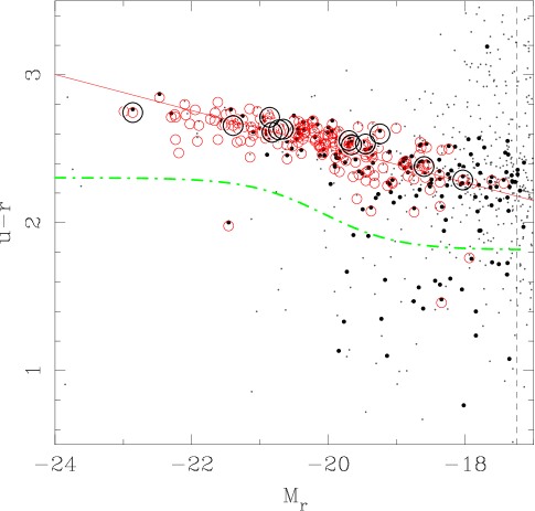
Figure 2: Sloan Digital Sky Survey (SDSS) DR6 (Adelman-McCarthy et al., 2007) colour–magnitude diagram of the central 1$\aas@@fstack{\circ}$5-diameter region of the Coma Cluster. Large black circles are the LRIS sample of galaxies presented here; red circles are early-type galaxies with line strengths analysed in the current work from several different samples (§2.4), some of which are outside the central region; black dots are galaxies with redshifts from DR6 placing them at the distance of the Coma Cluster; and small grey points are other galaxies in the same field without DR6 redshifts, assuming that they are also in the cluster. The dashed vertical line is the magnitude limit of SDSS spectroscopy; the dot-dashed green line demarcates the blue-red galaxy division of Baldry et al. (2004); and the red solid line is a fit to the brighter ($-23<M_{r}<-18$ mag), red, redshift-selected cluster members to guide the eye as to the location of the red sequence.

Twelve ETGs with $-22\la M_{b_{J}}\la-16$ (assuming a cluster velocity of $cz_{hel}=7007\;\mathrm{km\,s^{-1}}$, Hudson et al. 2001, and $H_{0}=72\;\mathrm{km\,s^{-1}}\mathrm{Mpc^{-1}}$, Freedman et al. 2001) were observed (Fig. 1; Table 1). Eight objects are typed as ‘S0’, two are typed as ‘E’, and one (GMP 3329=NGC 4874) is typed as ‘D’ by Dressler (1980b); the twelfth object, GMP 3565, is typed as ‘E/S0’ by P. van Dokkum in Beijersbergen et al. (2002). We therefore have observed an ETG sample, albeit one dominated by S0 galaxies. All of these galaxies lie on the cluster red sequence (Fig. 2).

Spectra were obtained in three consecutive 30-minute exposures on 1997 April 7 UT with the red side of LRIS (LRIS-B was not yet available), with seeing $\mathrm{FWHM}\approx 0\aas@@fstack{\prime\prime}8$ (as determined from the image in Fig. 1, taken directly before the spectrographic exposures), through clouds. A slit width of 1″ was used in conjunction with the 600 line $\mathrm{mm^{-1}}$ grating blazed at 5000 Å, giving a resolution of 4.4 Å FWHM ($\sigma=1.9$ Å, corresponding to a velocity dispersion resolution of $\sigma\sim 125\;\mathrm{km\,s^{-1}}$) and a wavelength coverage of typically 3500–6000 Å, depending on slit placement. Stellar spectra of five Lick/IDS standard G and K giant stars (HR 6018, HR 6770, HR 6872, HR 7429, and HR 7576) and four F9–G0 dwarfs (HD 157089, HD 160693, HR 5968, and HR 6458) also from the Lick/IDS stellar sample (Worthey et al., 1994) were observed on the same and subsequent nights through the LRIS 1″ long slit using the same grating. However, the wavelength coverage of the stellar spectra was restricted to the region 3500–5530 Å, preventing the calibration of indexes redder than Fe5406 present in the galaxy spectra (such as NaD).

2.1.1 Data reduction

The spectral data were reduced using a method that combined the geometric rectification procedures described by Kelson et al. (2000) and the sky-subtraction methodology of Kelson (2003). Namely, after basic calibrations (overscan correction, bias removal, dark correction, and flat field correction), a mapping of the geometric distortions and wavelength calibrations were made using a suite of Python scripts written by Dr. Kelson, following the precepts of Kelson et al. (2000). Arc lamps were used for wavelength calibration, which was adequate (but not perfect; see Appendix A) for wavelengths longer than 3900 Å. No slits were tilted, so geometric rectification was generally simple. However, these mappings were not applied until after the sky subtraction, for reasons detailed by Kelson (2003). For nine of the galaxies, sky spectra were interpolated from the slit edges, as the galaxies did not fill the slitlets, using Python scripts written by Dr. Kelson implementing his sky-subtraction method. However, for NGC 4874, which did fill its slitlet, and for D128 and NGC 4872, whose spectra were contaminated by that of NGC 4874, sky subtraction was performed first using the ‘sky’ information at the edge of their slitlets and then corrected by comparing this sky spectrum to the average sky from all other slitlets.

Extraction of one-dimensional spectra from the two-dimensional, sky-subtracted long-slit images involved a simultaneous variance-weighted extraction of the objects in a central aperture from all three images while preserving the best possible spectral resolution (Kelson, 2006). This involved using the geometric and wavelength mappings and interpolating the spectra to preserve the spectral resolution in the summed spectra. This extraction also serves as an excellent cosmic ray rejection scheme. Variance spectra were computed from the extracted signal and noise spectra. To understand the level of random errors, one-dimensional spectra were also extracted from each image separately (after a separate cosmic-ray cleaning step).

Various apertures were used to extract the spectra: apertures with equivalent circular diameters of $2\aas@@fstack{\prime\prime}0$, $2\aas@@fstack{\prime\prime}7$, $3\aas@@fstack{\prime\prime}2$, $3\aas@@fstack{\prime\prime}4$, $3\aas@@fstack{\prime\prime}6$, $3\aas@@fstack{\prime\prime}8$, $4\aas@@fstack{\prime\prime}5$, and a ‘physical’ aperture of $r_{e}/2$ diameter for all galaxies except GMP 3329 (=NGC 4874). For this galaxy, an aperture of $r_{e}/8$ diameter was used due its large projected size (note that an aperture of $r_{e}/8$ is too small to be extracted reliably for many of the galaxies in our sample: for example, $r_{e}/8=0\aas@@fstack{\prime\prime}33$ for GMP 3534; Table 1). These circular-aperture-equivalent extraction apertures were chosen to match closely existing line-strength measurements of these galaxies in the literature (see Appendix B). We use only indexes from the $2\aas@@fstack{\prime\prime}7$-diameter aperture in the analysis in this study, however. At the distance of the Coma Cluster and assuming again $H_{0}=72\;\mathrm{km\,s^{-1}}\mathrm{Mpc^{-1}}$, this corresponds to a physical diameter of 637 pc. We note that the results given here do not change significantly when using the ‘physical’ $r_{e}/2$ aperture instead of the 2$\aas@@fstack{\prime\prime}$7 aperture: for example, the mean ages of the LRIS galaxies (ignoring GMP 3329) are $\langle\log t\rangle=0.69\pm 0.02$ for the 2$\aas@@fstack{\prime\prime}$7 aperture and $\langle\log t\rangle=0.67\pm 0.02$ for the $r_{e}/2$ aperture. When comparing other studies to ours in the analysis, we use available gradient information to transform their indexes to an equivalent circular aperture of the same diameter ($2\aas@@fstack{\prime\prime}7$), when possible. We postpone discussion of the gradients in our data to future work.

To account for the transformation of the rectangular extraction aperture to an equivalent circular aperture, the extracted spectra were weighted by $|r\,\Delta r|$, where $r$ is the distance from the object centre to the object row being extracted and $\Delta r$ is the pixel width (cf. González, 1993). Note that the spectra were sub-sampled along the spatial direction during the extraction process to account for the geometric and wavelength distortions, so $\Delta r$ was typically less than one in pixel space. The variance spectra were weighted by $|r^{2}\Delta r|$ in order to preserve the noise properties.

Figure 3: Spectra of Coma ETGs through a central aperture of diameter $2\aas@@fstack{\prime\prime}7$. Each spectrum has been flux-calibrated and shifted to zero systemic velocity; no smoothing has been applied. The ‘noise’ around 5450 Å is the result of imperfect subtraction of the extremely bright [O i]$\lambda 5577$ night-sky line. The median S/N per $75\,\mathrm{km\,s^{-1}}$ pixel in the observed wavelength range 4285–5200 Å is given. See Fig. 18 for an expanded view in the restframe region 4800–5300 Å.

In order to remove the instrumental response function from the galaxies, flux standard stars can be used to calibrate the object spectra onto a relative flux scale. As the spectra were taken through clouds, it is not possible to calibrate them to an absolute flux scale. However, an absolute flux measurement is unnecessary when our purpose is to measure line-strength indexes, as these are relative measurements of the absorption line fluxes with respect to the level of the nearby continuum. The flux standard star BD$+33\degr 2642$ (Oke, 1990) was taken through both the longslit setup and slitless at different detector locations through the multislit setup to cover the full wavelength range. The extracted spectrum was first normalised by dividing by the median count level of the spectrum and then smoothed with a wavelet filter to derive a sensitivity curve for each observation of the flux standard. The flux-calibrated spectrum of BD$+33\degr 2642$ from Oke (1990) was also normalised and smoothed and then divided by the normalised, smoothed LRIS flux standard spectra to create a sensitivity spectrum $\mathcal{F}(\lambda)$. The sensitivity curves derived from slitless spectra taken at the most extreme positions perpendicular to the slit direction (i.e., at the largest wavelength spread) were combined into a single sensitivity spectrum after flat fielding by joining them at a convenient matching point in order to derive a sensitivity curve for the multislit spectra (which covered a larger wavelength span than the longslit spectra). The final fluxed spectra through the central $2\aas@@fstack{\prime\prime}7$-diameter equivalent circular aperture of the twelve galaxies observed are shown in Figure 3.

2.2 Velocities, velocity dispersions, and line strengths

To test the predictions made in §1, we require both the stellar population parameters of ETGs in the Coma cluster and their velocity dispersions. We measure line strengths of the galaxies and compare them with stellar population models such as Worthey (1994). Therefore we must know the systemic velocity of the object to place the bandpasses on the spectra properly and we must know the velocity dispersion of the object (e.g., González, 1993; Trager et al., 1998) to place line strengths onto the Lick/IDS stellar system on which the models are defined (see §2.3 and Appendix A).

2.2.1 Systemic velocities and velocity dispersions

We begin with a discussion of the determination of systemic velocities $v$ and velocity dispersions $\sigma$. Following Kelson et al. (2000, and earlier work by ), we first build a pixel-space model $M$ of the galaxy spectrum $G$ from a stellar or stellar population model template $T$ convolved with a broadening function $B(v,\sigma)$: $M=B(v,\sigma)\circ T$. In its simplest form, we want to minimise the residuals between the galaxy and model $\chi^{2}=|G-M|^{2}=|G-B\circ T|^{2}$. However, as both noise and continuum mismatches (both multiplicative and additive) between the galaxy and model will be present in any practical situation, we instead write

$$\chi^{2}=\left|{\left\{G-\left[P_{M}(B\circ T)+\sum_{j=0}^{K}a_{j}H_{j}\right]\right\}\times W}\right|^{2}.$$ (1)

Here $P_{M}$ is a multiplicative polynomial used to remove large-scale fluxing differences between the galaxy and template spectra (which here is not continuum-subtracted before fitting). In this study, we use a fourth-order Legendre polynomial for $P_{M}$ to remove the multiplicative continuum mismatch between the galaxy and template. The zeroth order term of $P_{M}$ is equivalent to $\gamma$, the ‘line strength parameter’, found in the literature (Kelson et al., 2000). The additive continuum mismatch is controlled by the collection of sines and cosines $H_{j}$ up to order $K$. This is effectively a low-pass filter used to minimise continuum mismatch. We use $K=1.5\Delta\lambda/100\,$Å in the current study, where $\Delta\lambda$ is the wavelength coverage (in the restframe) of the fitting region. $W$ is the pixel-space weight vector, which can be a combination of the variance spectrum and any masking of ‘bad’ regions (e.g., poorly-subtracted strong night sky lines) desired. (Note that we ignore the additive polynomial functions described by Kelson et al. 2000.) The coefficients of $P_{M}$ and $H_{j}$ as well as the desired quantities $v$ and $\sigma$ are solved for in the fitting process, which is described in detail by Kelson et al. (2000). Dr. Kelson has kindly provided us with LOSVD, a Python script that implements this algorithm.

For ten galaxies, the K1 giant star HR 6018 proved to be the best velocity dispersion template, as judged by the reduced-$\chi^{2}$ of the fit. For the galaxies GMP 3534 and GMP 3565, the G0 dwarf HR 6458 provided a somewhat better fit. Tests using the Vazdekis (1999) spectral models as templates suggest that the use of an well-matched template never changes the derived velocity dispersion by more than 2 per cent. This is negligible for our purposes of correcting the Lick/IDS line strengths onto the stellar system (below) or for determining correlations of velocity dispersion with stellar population parameters. We fit the galaxy spectra in the observed wavelength region 4285–5200 Å (roughly 4180–5080 Å in the rest frame, and therefore $K=13$), which covers the strong G band feature, H$\gamma$, $\mathrm{H}\beta$, and many other weaker lines. We do not fit the MgH and Mg i triplet region at 5100–5300 Å in the rest frame due to the strong but variable continuum depression from the dense forest of MgH lines. In all cases, the template stars were set to zero recessional velocity and derived velocities were corrected to heliocentric velocities.

We note that for three galaxies, GMP 3291, GMP 3534, and GMP 3565, the measured velocity dispersions are significantly below the resolution limit of $\sim 125\,\mathrm{km\,s^{-1}}$ and thus may be significantly in error, even given the high signal-to-noise of the present spectra. Two of these galaxies, GMP 3534 and GMP 3565, were recently observed at $\sim 35\,\mathrm{km\,s^{-1}}$ resolution by Matković & Guzmán (2005), and our measured velocity dispersions match theirs within the $1\sigma$ joint errors for each of these two objects. While this does not guarantee that our velocity dispersion measurement of GMP 3291 is correct, it does suggest that our measurement is not far from the true value (see Appendix B for more detailed comparisons).

2.3 Line strengths on the Lick/IDS system

Once the systemic velocity of the object is known, the bandpasses can be placed on the spectrum and line strengths can be measured. We give a brief description here and leave a detailed description for Appendix A.

First, any emission lines in the spectra are corrected using GANDALF (Sarzi et al., 2006). These corrections only affect the Fe5015 indexes, as significant $\mathrm{H}\beta$ emission is not detected using this procedure in any galaxy, even though significant [Oiii] emission is detected in ten of the twelve. We therefore use the uncorrected $\mathrm{H}\beta$ strengths throughout this paper; we discuss this further in §4.2.1 below. Then the spectra are smoothed to the Lick/IDS resolution, which varies with wavelength (Worthey & Ottaviani, 1997). Next, the wavelengths of the Lick/IDS index bandpasses are defined using a template star. These bandpasses are then shifted to match the velocity of each object. Corrections for non-zero velocity dispersion are made for each index of each galaxy. Stellar indexes are then compared to those of the same stars in the Lick/IDS stellar library (Worthey et al., 1994) to determine the offsets required to bring each index onto the Lick/IDS system.

Landscape table to go here

Table 2:

The fully-corrected (emission-, Lick/IDS system-, and velocity dispersion-corrected) line strengths for the $2\aas@@fstack{\prime\prime}7$-diameter equivalent circular aperture are given in Table 2. We summarise this subsection (and by extension Appendixes A and B) by stating that the LRIS data are fully corrected and well-calibrated onto the Lick/IDS system for all indexes of interest to the current study.

2.4 Literature data: Coma and ‘field’ galaxies

We briefly describe other high-quality line strength data of Coma Cluster galaxies available in the literature. A full comparison of these data with our LRIS data is given in Appendix B.

Table 3: Literature data sources of absorption-line strengths in the Coma Cluster on the Lick/IDS system

		Effective circular
Reference	Abbreviation	aperture diameter
Dressler (1984)	D84	4$\aas@@fstack{\prime\prime}$5
Fisher, Franx, & Illingworth (1995)	FFI	3$\aas@@fstack{\prime\prime}$2
Guzman et al. (1992)	G92	3$\aas@@fstack{\prime\prime}$8
Hudson et al. (2001)	H01	2$\aas@@fstack{\prime\prime}$7
Jørgensen (1999)	J99	3$\aas@@fstack{\prime\prime}$4
Kuntschner et al. (2001)	K01	3$\aas@@fstack{\prime\prime}$6
Matković & Guzmán (2005)	MG05	3$\aas@@fstack{\prime\prime}$0
Mehlert et al. (2000)	M00	2$\aas@@fstack{\prime\prime}$7
Moore et al. (2002)	M02	2$\aas@@fstack{\prime\prime}$7
Nelan et al. (2005)	NFPS	2$\aas@@fstack{\prime\prime}$0
Poggianti et al. (2001)	P01	2$\aas@@fstack{\prime\prime}$7
Sánchez-Blázquez et al. (2006b)	SB06	2$\aas@@fstack{\prime\prime}$7
Terlevich et al. (1999)	T99	2$\aas@@fstack{\prime\prime}$0
Trager et al. (1998);	IDS	2$\aas@@fstack{\prime\prime}$7
Lee & Worthey (2005)

In Table 3 we list all of the sources of absorption-line strength data calibrated onto the Lick/IDS system (as well as heliocentric velocities and velocity dispersions) for the Coma Cluster that we have found in the literature. For the Lick/IDS (IDS) sample, the higher-order Balmer line strengths of NGC 4864 and NGC 4874 were taken from Lee & Worthey (2005). Most of these line strengths were measured through fibres of various apertures, or in the case of the Lick/IDS sample, a rectangular slit; in those cases where long slit data were obtained, an equivalent circular aperture was synthesised from published gradient data. For the Moore et al. (2002) sample, $\mathrm{H}\beta$ line strengths were corrected for emission using the equivalent width of the [O iii]$\lambda 5007$ Å line following the procedure detailed in Trager et al. (2000a); that is, we correct $\mathrm{H}\beta$ by adding $-0.6\times\mathrm{EW([O\,\textsc{iii}])}$ when [Oiii] is in emission (i.e., $\mathrm{EW([O\,\textsc{iii}])}<0$). We note that this correction was not made for the Jørgensen (1999), Mehlert et al. (2000), Nelan et al. (2005), or Sánchez-Blázquez et al. (2006b) samples, nor even our own LRIS sample; we return this point in §5.3 below. In Table 3 in Appendix B we present the line strengths and stellar population parameters for all Coma Cluster galaxies for which line strengths were available in the literature that were taken through or could be synthesised to form a $2\aas@@fstack{\prime\prime}7$-diameter aperture.

We also use the samples of González (1993, field and Virgo cluster ellipticals), Fisher, Franx, & Illingworth (1996, field and Virgo cluster S0’s), and Kuntschner (2000, Fornax Cluster ETGs) in our analysis. In each case we computed line strengths through synthesised apertures of diameter $2\aas@@fstack{\prime\prime}7$ projected to the distance of Coma using the published gradient data. That is, we measured line strengths through a fixed physical aperture of radius $637\;\mathrm{pc}$ (assuming $H_{0}=72\;\mathrm{km\,s^{-1}}\,\mathrm{Mpc^{-1}}$, as above).We have combined these three samples, excluding ETGs in the Virgo Cluster, to create a low-density environment sample that we refer to as our ‘field’ sample. We can then directly compare the stellar populations of these ETGs in less-dense environments to those of Coma ETGs.

2.5 Galaxy masses and mass-to-light ratios

Table 4: Virial $M_{\mathrm{vir}}$ mass-to-light ratios and masses of the LRIS sample galaxies

GMP	$\log M_{\mathrm{vir}}/L_{B}$	$\log M_{\mathrm{vir}}$
3254	$0.66\pm 0.08$	$10.04\pm 0.08$
3269	$0.36\pm 0.09$	$9.86\pm 0.09$
3291	$0.55\pm 0.11$	$10.02\pm 0.11$
3329	$1.07\pm 0.08$	$11.90\pm 0.08$
3352	$0.44\pm 0.08$	$10.49\pm 0.08$
3367	$0.56\pm 0.08$	$10.69\pm 0.08$
3414	$0.49\pm 0.08$	$10.66\pm 0.08$
3484	$0.37\pm 0.08$	$9.98\pm 0.08$
3534	$0.24\pm 0.12$	$9.52\pm 0.12$
3565	$0.33\pm 0.23$	$9.18\pm 0.23$
3639	$0.41\pm 0.08$	$10.56\pm 0.08$
3664	$0.67\pm 0.08$	$10.89\pm 0.08$

We are further interested in the masses and mass-to-light ratios of ETGs in the Coma Cluster to examine the variation of line strengths and stellar population parameters as a function of mass and to probe for complex star-formation histories. We have determined a ‘virial mass’ $M_{\mathrm{vir}}=500\,\sigma_{e}^{2}r_{e}\,\mathrm{M_{\odot}}$ (Cappellari et al., 2006), where $\sigma_{e}$ is the light-weighted velocity dispersion within the effective radius in $\mathrm{km\,s^{-1}}$, computed as $\sigma_{e}=\sigma_{2\aas@@fstack{\prime\prime}7}[r_{e}(\arcsec)/2\aas@@fstack{\prime\prime}7]^{-0.066}$, and $r_{e}$ is the effective radius in parsecs derived from Jørgensen & Franx (1994, or Table 1 when necessary). The virial mass-to-light $M_{\mathrm{vir}}/L_{B}$ ratio in the $B$-band is computed from $M_{\mathrm{vir}}$ using $L_{B}$. We have corrected $B$-band magnitudes for our galaxies from Eisenhardt et al. (2007) using $k$-corrections appropriate for a 13 Gyr-old, solar-metallicity SSP (Bruzual & Charlot, 2003) model and using extinctions computed using Schlegel, Finkbeiner, & Davis (1998) for the KPNO $B$ filter and finally assumed a distance modulus of 34.94 to the Coma Cluster to determine $L_{B}$. We do not use the direct scaling of $M/L$ with $\sigma_{e}$ from Cappellari et al. (2006, their Eq. (7)), as the galaxies with the lowest velocity dispersions in our sample have resulting mass-to-light ratios much lower than their stellar populations would suggest, which is unphysical.

3 Derivation of stellar population parameters

Our methodology for inferring stellar population parameters from absorption-line strengths has changed since Trager et al. (2000a, b, 2005) due to improvements in the models and to increasing computer speeds. We first describe our new models and then the method used to infer SSP-equivalent (single-stellar-population-equivalent) parameters from the observed line strengths. By ‘SSP-equivalent’, we mean that the stellar population parameters we determine are those the object would have if formed at a single age with a single chemical composition. As discussed at length in Paper II and in §5.1, we do not believe that early-type galaxies are composed of single stellar populations. For convenience and because of the degeneracies discussed in Worthey (1994), Paper II and Serra & Trager (2007, among many others), our analysis is however conducted using SSP-equivalent parameters.

3.1 Models

In the current paper we follow our past practise and analyse stellar populations with the aid of the Worthey (1994) models. We have however improved our previous models and methods in two ways: (1) the treatment of non-solar abundance ratios has been improved, and (2) the ‘grid inversion’ scheme used to infer stellar population parameters in this paper is a significant improvement on our previous scheme.

The first major improvement in the method is the improved treatment of the effect of non-solar abundance ratios on the line strengths. In the past, we (Trager et al., 2000a, hereafter Paper I) and others (e.g., Thomas, Maraston, & Bender, 2003, hereafter TMB03) used the response functions of Tripicco & Bell (1995) to account for these effects in the original 21 Lick/IDS indexes (Worthey et al., 1994). The Tripicco & Bell (1995) response functions were computed for only three stars along a 5 Gyr old, solar-metallicity isochrone, leaving some doubt about their applicability to significantly different populations. These were superseded by the response functions of Korn et al. (2005), who used three stars on 5 Gyr isochrones at many different metallicities and also computed the response functions for the higher-order Balmer-line indexes of Worthey & Ottaviani (1997).

Recently, Worthey (priv. comm.) has produced new response functions for non-solar abundance ratios. These are based on newly-computed synthetic spectra of model stellar atmospheres for all of the stars in all of the isochrones in the ‘vanilla’ W94 (i.e., using original W94 isochrones) and the ‘Padova’ W94 models (i.e., using the Bertelli et al. 1994 isochrones). One element at a time is altered in each spectrum, extending the work of Serven, Worthey, & Briley (2005). Each new spectrum is subtracted from the synthetic scaled-solar spectrum to compute a response function for each star along the isochrone; these are then summed to alter the model line strengths for each single-stellar-population model. Dr. Worthey kindly sent us model indexes for an elemental mixture of fixed $\mathrm{[E/Fe]}=+0.3$ (mixture 4 of Paper I) for the full grids of both the W94 and Padova models. Because of the close similarity of the Padova1994 plus Salpeter IMF version of the Bruzual & Charlot (2003, hereafter ‘BC03’) models and the Padova W94 models, we can use the deviation of the indexes of the $\mathrm{[E/Fe]}=+0.3$ Padova W94 models from the scaled-solar mixture Padova W94 models to correct the BC03 models for non-solar abundance ratios. We do not give detailed results for stellar populations inferred from the ‘Padova’ W94 and BC03 models in this paper. However, we will point out the ranges in stellar population parameters that result from using different models when necessary, as the entire analysis has been carried out with the Padova W94 and BC03 models in parallel with the vanilla W94 models.

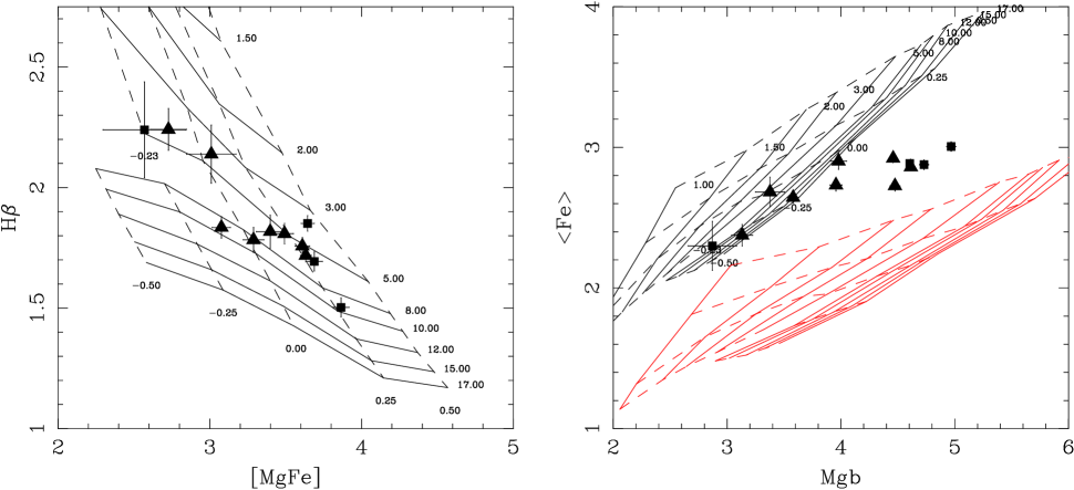
Figure 4: Stellar populations of Coma ETGs observed with LRIS in ($\mathrm{H}\beta$, $[\mathrm{MgFe}]$) and ($\mathrm{Mg}\,b$, $\langle\mathrm{Fe}\rangle$) space, where $[\mathrm{MgFe}]=\sqrt{\mathrm{Mg}\,b\times\langle\mathrm{Fe}\rangle}$ and $\langle\mathrm{Fe}\rangle=(\mathrm{Fe5270}+\mathrm{Fe5335})/2$. Line strengths in this figure are measured through the synthesised $2\aas@@fstack{\prime\prime}7$-diameter aperture. Triangles are S0’s, squares are ellipticals. Model grids come from the vanilla Worthey (1994) models, modified for $\mathrm{[E/Fe]}$ as described in the §3.1. In both panels, solid lines are isochrones (constant age) and dashed lines are isofers (constant metallicity $\mathrm{[Z/H]}$). In the left panels, the models are for solar $\mathrm{[E/Fe]}$; models with higher $\mathrm{[E/Fe]}$ have slightly lower $\mathrm{H}\beta$ but similar $[\mathrm{MgFe}]$. Therefore this an appropriate grid from which to visually assess age and metallicity, although accurate determinations are made in ($\mathrm{H}\beta$, $\mathrm{Mg}\,b$, Fe5270, Fe5335) space (see text). In the right panel, grids have $\mathrm{[E/Fe]}=0$, $+0.3$ (upper and lower, respectively). This is an appropriate diagram from which to visually asses $\mathrm{[E/Fe]}$.

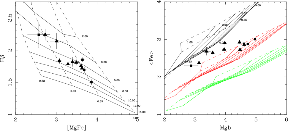
Figure 5: As for Figure 4, but here the grids are those of TMB03, as modified using the $\mathrm{[\alpha/Fe]}$ responses of Korn et al. (2005). Although the inferred metallicities and enhancement ratios differ in comparison to the models used in the current work, the ages inferred from the $[\mathrm{MgFe}]$–$\mathrm{H}\beta$ diagram (left) are very similar, showing that our preferred model is not the source of the young average age we find.

We show the new models, with our Coma Cluster ETG data superimposed, in Figure 4. These new $\mathrm{[E/Fe]}=+0.3$ grids fall between the $\mathrm{[E/Fe]}=+0.3$ and $\mathrm{[E/Fe]}=+0.5$ grids in, say, $\mathrm{Mg}\,b$ versus $\langle\mathrm{Fe}\rangle$, of older models based on Tripicco & Bell (1995) or Korn et al. (2005) so that our new results tend to have smaller $\mathrm{[E/Fe]}$ at high $\mathrm{[E/Fe]}$ than previous studies (compare Fig. 4 with Fig. 5). For the LRIS sample, we find

$$\log t_{\mathrm{new}} = (1.16\pm 0.22)\log t_{\mathrm{Paper\ I}}-(0.21\pm 0.03)$$

$$\mathrm{[Z/H]}_{\mathrm{new}} = (1.24\pm 0.10)\mathrm{[Z/H]}_{\mathrm{Paper\ I}}+(0.04\pm 0.02)$$

$$\mathrm{[E/Fe]}_{\mathrm{new}} = (0.87\pm 0.08)\mathrm{[E/Fe]}_{\mathrm{Paper\ I}}+(0.00\pm 0.01),$$

where the Paper I values were computed using the W94 models and the Tripicco & Bell (1995) responses. These relations suggest that, across the board, our ages are somewhat lower (younger) at all ages, metallicities are increasingly higher at high $\mathrm{[Z/H]}$, and as expected, enhancement ratios lower at high $\mathrm{[E/Fe]}$ in the new models than in those presented in Paper I. We also show the models of TMB03 (as modified using the $\mathrm{[\alpha/Fe]}$ responses of Korn et al., 2005) and our Coma Cluster ETG data in Figure 5 to demonstrate that the newly-modified W94 models predict nearly the same ages as the TMB03 models, even though they predict lower metallicities and enhancement ratios. We use our new models for all comparison with previous studies. That is, we compute SSP-equivalent parameters using our present models from the line strengths given in previous studies when comparisons are made.

Our method is not self-consistent, as we are manipulating the atmospheric parameters of the stars of interest and not their interior parameters, as discussed in Paper I. That is, we are not altering the isochrones of the Worthey (1994) or the Bruzual & Charlot (2003) models to accommodate changes in $\mathrm{[E/Fe]}$ (or, more generally, $[X_{j}/\mathrm{Fe}]$). Proctor & Sansom (2002) have examined the methodology of Paper I in light of $\alpha$-enhanced isochrones from the Padova group (Salasnich et al., 2000). They note that at high metallicity, the Salasnich et al. (2000) isochrones are not significantly changed by increasing $\mathrm{[E/Fe]}$ at fixed $\mathrm{[Fe/H]}$; therefore the isochrones appear to depend on $\mathrm{[Fe/H]}$, not $\mathrm{[Z/H]}$, as we have assumed. Proctor & Sansom therefore choose to enhance all the elements by $\mathrm{[E/Fe]}$ except the Fe-like elements Fe, Ca, and Cr, which are kept at their original $\mathrm{[Fe/H]}$ level. This is in contrast to our method described in Paper I, where we assumed that the isochrones depend on the total metallicity $\mathrm{[Z/H]}$, as discussed in §3.1.2 and §5.4 in that paper, and thus some elemental abundances are enhanced and others decreased to keep $\mathrm{[Z/H]}$ in balance. The Proctor & Sansom method tends to increase the ages of the galaxies with the highest $\mathrm{[E/Fe]}$ compared with our method – for galaxies with ages $\log t\ga 0.6$, the increase is $\Delta\log t\sim 0.25$ (cf. their Fig. 11) – but barely affects the other stellar population parameters. We agree that our assumptions need updating, but we currently prefer to use our original assumption that isochrone shapes are governed by $\mathrm{[Z/H]}$ and wait for self-consistent stellar population models in which indexes and isochrones are corrected for $\mathrm{[E/Fe]}$ in the same way (see the discussion in TMB03 and attempts by Weiss, Peletier, & Matteucci 1995; Thomas & Maraston 2003; Lee & Worthey 2005; and Schiavon 2007). Note moreover the recent suggestion by Weiss et al. (2006) that the Salasnich et al. (2000) isochrones are untrustworthy because of errors in the low-temperature opacities; this will certainly affect the conclusions of Proctor & Sansom (2002), Thomas & Maraston (2003), and Schiavon (2007).

Finally, we have not (yet) corrected the models for the so-called $\mathrm{[\alpha/Fe]}$-bias inherent in the fitting functions (TMB03). This ‘bias’ is however only strong ($\mathrm{[\alpha/Fe]_{intrinsic}}>0.1$ dex) when $\mathrm{[Fe/H]}<-0.33$ dex, uncommon in ETGs. Such a low metallicity is not seen in the ETGs in LRIS sample (the lowest metallicity is that of GMP 3565, which has $\mathrm{[Z/H]}=-0.25$ dex).

3.2 Method

We have also improved the scheme (‘grid inversion’) by which line strengths are fit to models and therefore stellar population parameters and errors are determined.

Previously we created large, finely-spaced grids in ($\log t$, $\mathrm{[Z/H]}$, $\mathrm{[E/Fe]}$) space and searched the corresponding ($\mathrm{H}\beta$, $\mathrm{Mg}\,b$, $\langle\mathrm{Fe}\rangle$) grids using a minimal-distance statistic to find the best-fitting stellar population parameters (Paper I). Errors were determined by altering each line strength by $1\sigma$ in turn and searching the grids again to find the maximum deviation in each stellar population parameter.

Given the ever-improving speed and memory of modern computers, such a method is no longer necessary. We now determine stellar population parameters directly using a non-linear least-squares code based on the Levenberg-Marquardt algorithm in which the stellar population models described above are linearly interpolated in ($\log t$, $\mathrm{[Z/H]}$, $\mathrm{[E/Fe]}$) on the fly. Confidence intervals are computed by taking the dispersion of stellar population parameters from $10^{4}$ Monte Carlo trials using the errors of the observed line strengths (Table 2), assuming Gaussian error distributions. At the same time, we have extended the method from ($\mathrm{H}\beta$, $\mathrm{Mg}\,b$, $\langle\mathrm{Fe}\rangle$) distributions to any combination of indexes; for example, determining stellar populations when $\mathrm{C}_{2}4668$ is substituted for $\mathrm{Mg}\,b$ or $\mathrm{H}\delta_{A}$ for $\mathrm{H}\beta$. In fact, we now use Fe5270 and Fe5335 in the fitting process separately rather than $\langle\mathrm{Fe}\rangle$. We display the data in the ($\mathrm{H}\beta$, $[\mathrm{MgFe}]$) and ($\mathrm{Mg}\,b$, $\langle\mathrm{Fe}\rangle$) planes, because these planes are respectively sensitive to age and metallicity (but mostly insensitive to $\mathrm{[E/Fe]}$) and sensitive to $\mathrm{[E/Fe]}$ (e.g., Fig. 4; TMB03). We do not determine stellar population parameters from these planes. We also compute expected line strengths and optical through near-infrared colours (and their errors) based on the computed stellar population parameters. We have tested this scheme on the González (1993) data presented in Papers I and II and found it to reproduce very closely the stellar population parameters derived there when using models similar to those used in those papers.

3.3 A check of the models and method

As a sanity check of the above changes to the models and method, we have determined the age, metallicity and enhancement ratio of the galactic open cluster M67 using the Lick/IDS indexes given by Schiavon, Caldwell, & Rose (2004a). We find $t=4.1\pm 0.7$ Gyr, $\mathrm{[Z/H]}=-0.13\pm 0.06$ dex, and $\mathrm{[E/Fe]}=0.01\pm 0.03$ dex (when ignoring blue straggler stars), in excellent agreement with both the colour-magnitude diagram turnoff age (3.5 Gyr) and spectroscopic abundances ($\mathrm{[Z/H]}\approx\mathrm{[E/Fe]}\approx 0$ dex) as well as the model ages and abundances ($t=3.5\pm 0.5$ Gyr, $\mathrm{[Z/H]}=0.0\pm 0.1$ dex, $\mathrm{[Mg/Fe]}=-0.05\pm 0.05$) determined by Schiavon et al. (2004a). We are therefore confident that we can accurately and precisely recover the stellar population parameters of intermediate-aged, solar-composition single stellar populations.

4 The stellar populations of early-type galaxies in the Coma Cluster

We now explore the resulting stellar population parameters of ETGs in the Coma Cluster. In the following, except where indicated, the terms ‘age’ ($t$), ‘metallicity’ ($\mathrm{[Z/H]}$), and ‘enhancement ratio’ ($\mathrm{[E/Fe]}$) always refer to the SSP-equivalent parameters. We test our three predictions of §1 using the stellar population parameters and their correlations with velocity dispersion and mass.

4.1 Line-strength distributions

In Figure 4 we plot the distribution of $\mathrm{H}\beta$, $\mathrm{Mg}\,b$, $\langle\mathrm{Fe}\rangle$ line strengths of our twelve Coma Cluster galaxies. Before discussing results based on stellar population parameters determined from the grid inversion, three major points can be read directly from this diagram. First, these objects span a relatively narrow range in age (less than a factor of 3, or less than 0.5 in $\log t$). At least 8 of the 12 galaxies have nearly-identical ages around 5 Gyr. Note that these ages from this plot will not precisely agree with the parameters given in Table 5 below due to lower $\mathrm{H}\beta$ at fixed age for larger $\mathrm{[E/Fe]}$. This means that high-$\mathrm{[E/Fe]}$ galaxies will be slightly younger when using our age-dating method than ages read directly from the plot. Second, the galaxies span a large range in metallicity $\mathrm{[Z/H]}$, about 0.5 dex, as can be seen from the left-hand panel, centred on a value of $\sim 1.5$ times the solar value. Third, the $\mathrm{[E/Fe]}$ ratios vary between the solar value and $+0.15$ dex or so for the newly-modified W94 models, as can be seen from the right-hand panel. We note here that differences between models cause subtle bulk changes in age and metallicity, but the overall trends are not grossly affected by the choice of model.

4.2 Stellar population parameter distributions

Table 5: SSP-equivalent stellar population parameters of Coma Cluster galaxies through the 2$\aas@@fstack{\prime\prime}$7-diameter aperture using ($\mathrm{H}\beta$, $\mathrm{Mg}\,b$, Fe5270, Fe5335)

GMP	$\log(t/\mathrm{Gyr})$	$t$ (Gyr)	$\mathrm{[Z/H]}$	$\mathrm{[E/Fe]}$
3254	$0.82_{-0.14}^{+0.10}$	$6.6_{-1.9}^{+1.7}$	$0.16_{-0.05}^{+0.07}$	$0.05_{-0.01}^{+0.03}$
3269	$0.96_{-0.05}^{+0.05}$	$9.2_{-1.1}^{+1.2}$	$-0.08_{-0.01}^{+0.04}$	$0.03_{-0.01}^{+0.01}$
3291	$0.61_{-0.31}^{+0.17}$	$4.1_{-2.1}^{+2.0}$	$0.07_{-0.10}^{+0.13}$	$0.03_{-0.03}^{+0.04}$
3329	$0.90_{-0.04}^{+0.05}$	$7.9_{-0.7}^{+1.0}$	$0.38_{-0.01}^{+0.04}$	$0.17_{-0.01}^{+0.01}$
3352	$0.68_{-0.02}^{+0.04}$	$4.8_{-0.2}^{+0.4}$	$0.36_{-0.02}^{+0.02}$	$0.18_{-0.01}^{+0.01}$
3367	$0.66_{-0.04}^{+0.04}$	$4.5_{-0.4}^{+0.4}$	$0.32_{-0.04}^{+0.04}$	$0.19_{-0.01}^{+0.01}$
3414	$0.66_{-0.02}^{+0.04}$	$4.5_{-0.2}^{+0.4}$	$0.36_{-0.04}^{+0.04}$	$0.14_{-0.01}^{+0.01}$
3484	$0.89_{-0.05}^{+0.08}$	$7.8_{-0.9}^{+1.6}$	$0.07_{-0.04}^{+0.05}$	$0.08_{-0.01}^{+0.01}$
3534	$0.66_{-0.07}^{+0.07}$	$4.6_{-0.7}^{+0.8}$	$-0.09_{-0.02}^{+0.05}$	$0.06_{-0.03}^{+0.03}$
3565	$0.70_{-0.22}^{+0.16}$	$5.0_{-2.0}^{+2.2}$	$-0.25_{-0.08}^{+0.17}$	$0.00_{-0.04}^{+0.09}$
3639	$0.48_{-0.02}^{+0.04}$	$3.0_{-0.2}^{+0.3}$	$0.54_{-0.01}^{+0.04}$	$0.20_{-0.01}^{+0.01}$
3664	$0.67_{-0.05}^{+0.05}$	$4.7_{-0.5}^{+0.6}$	$0.41_{-0.04}^{+0.05}$	$0.19_{-0.01}^{+0.01}$

Note. – Errors are 68 per cent confidence intervals marginalised over the other parameters. Errors are determined from observational uncertainties only and do not take into account systematic uncertainties.

Figure 6: The summed and individual probability distributions of stellar population parameters for galaxies in the centre of the Coma Cluster, based on the ($\mathrm{H}\beta$, $\mathrm{Mg}\,b$, Fe5270, Fe5335) indexes. Each galaxy’s probability distribution in each parameter is shown in a different colour; the (re-binned) sum is shown in black. Jagged features in the distributions arise from edge effects in the models. These summed distributions in these panels can be thought of as histograms smoothed by the errors in the parameters.

In Table 5 we present the stellar population parameters for the twelve Coma Cluster galaxies through the 2$\aas@@fstack{\prime\prime}$7-diameter synthesised aperture based on the ($\mathrm{H}\beta$, $\mathrm{Mg}\,b$, Fe5270, Fe5335) indexes. Figure 6 shows the distribution of stellar population parameters, shown as the probability distributions of each parameter marginalised over all other parameters and their sum. Galaxies in this figure are distributed as expected from Figure 4.

Examining these distributions and Table 5 in detail, we find that eight to ten of the twelve ETGs in this sample have nearly the same age. Discarding the two most divergent galaxies – GMP 3269 and GMP 3639 – the mean age of the ten remaining ETGs is $\mu_{\log t}=0.72\pm 0.02$ dex ($5.2\pm 0.2$ Gyr). To quantify the age scatter, we compute a reduced $\chi^{2}$ for the ETG ages:

$$\chi^{2}_{\nu}=\frac{1}{N-1}\sum_{i=1}^{N}\left(\frac{\log t_{i}-\langle\log t\rangle}{\sigma_{i}}\right),$$ (2)

where $\langle\log t\rangle=\mu$ is the weighted mean (logarithmic) age for the $N=10$ galaxies being considered and the $N-1$ term in the denominator arises from the fact that the we have computed $\mu$ from the distribution of $\log t$ itself. We have used the central value and scale (roughly $\sigma$) of the marginalised age distribution given by the biweight estimator (see, e.g., Beers, Flynn, & Gebhardt, 1990) to simplify the calculation. The biweight ages and best-fitting ages are nearly identical; the biweight scales closely match the half-width of the (68 per cent) confidence intervals but are assumed to be symmetric about the biweight age, unlike the confidence intervals. We find a reduced $\chi^{2}_{\nu}=2.4$ for the age residuals, or a 1 per cent chance of being consistent with no age spread (although see below). To determine the amount of permissible internal age scatter, we compute $\sigma_{\log t}(\mathrm{int})=\sqrt{V-N\sigma^{2}_{\mu}}$, where the sample variance $V=\sum_{i}(x_{i}-\mu)^{2}/(N-1)$. The maximum internal age scatter is then 0.11 dex (1.3 Gyr). The two deviant ETGs, GMP 3269 and GMP 3639 are notable for having the largest peculiar motions of the sample. GMP 3639 has a peculiar motion of $\approx-2200\,\mathrm{km\,s^{-1}}$, more than $2\sigma_{cl}$ [$\sigma_{cl}(\mathrm{Coma})=1021\,\mathrm{km\,s^{-1}}$, Smith et al. 2004] in front of the cluster, while GMP 3269 has a peculiar motion of $\approx 1000\,\mathrm{km\,s^{-1}}$ to the rear of the cluster. If these ETGs are assumed to be true cluster members, the mean age decreases negligibly to $\mu_{\log t}=0.71\pm 0.02$ dex ($5.1\pm 0.2$ Gyr) and the internal age spread increases to 0.14 dex (1.7 Gyr). We conclude therefore that ten of the twelve ETGs in this sample have the same age to within 1 Gyr and that including the remaining two (at least one of which may be an interloper) increases the typical age spread to only 1.7 Gyr.

Table 6: Kolmogorov-Smirnov probabilities for single-aged populations

$\log t$	Age	Sample
(dex)	(Gyr)	LRIS	J99	M00	M02	NFPS	SB06	Field
0.1	1.26	$0.002_{-0.002}^{+0.008}$
0.2	1.58
0.3	2.00		$0.014_{-0.012}^{+0.032}$
0.4	2.51		$\mathit{0.253}_{-0.180}^{+0.338}$
0.5	3.16	$0.001_{-0.000}^{+0.002}$	$\mathit{0.499}_{-0.332}^{+0.365}$	$0.002_{-0.002}^{+0.005}$
0.6	3.98	$0.011_{-0.008}^{+0.023}$	$0.050_{-0.040}^{+0.116}$	$0.030_{-0.027}^{+0.085}$
0.7	5.01	$\mathit{0.614_{-0.365}^{+0.234}}$	$0.001_{-0.001}^{+0.002}$	$\mathit{0.423}_{-0.308}^{+0.260}$	$0.044_{-0.032}^{+0.058}$			$0.040_{-0.021}^{+0.037}$
0.8	6.31	$0.113_{-0.079}^{+0.136}$		$\mathit{0.652}_{-0.332}^{+0.215}$	$0.006_{-0.005}^{+0.005}$		$0.001_{-0.001}^{+0.002}$	$0.023_{-0.017}^{+0.026}$
0.9	7.94	$0.023_{-0.013}^{+0.011}$		$\mathit{0.399}_{-0.284}^{+0.284}$			$0.046_{-0.039}^{+0.069}$
1.0	10.00	$0.001_{-0.001}^{+0.001}$		$\mathit{0.126}_{-0.110}^{+0.194}$		$0.043_{-0.035}^{+0.058}$	$\mathit{0.277}_{-0.162}^{+0.209}$
1.1	12.59			$0.004_{-0.003}^{+0.012}$		$0.001_{-0.001}^{+0.002}$	$\mathit{0.300}_{-0.185}^{+0.186}$
1.2	15.85						$0.028_{-0.025}^{+0.087}$

Entries in italics are those that are consistent with a constant age population. Errors are the extrema of the 68 per cent confidence intervals, determined from 100 realisations at the given age (see text). Sample names are defined in Table 3.

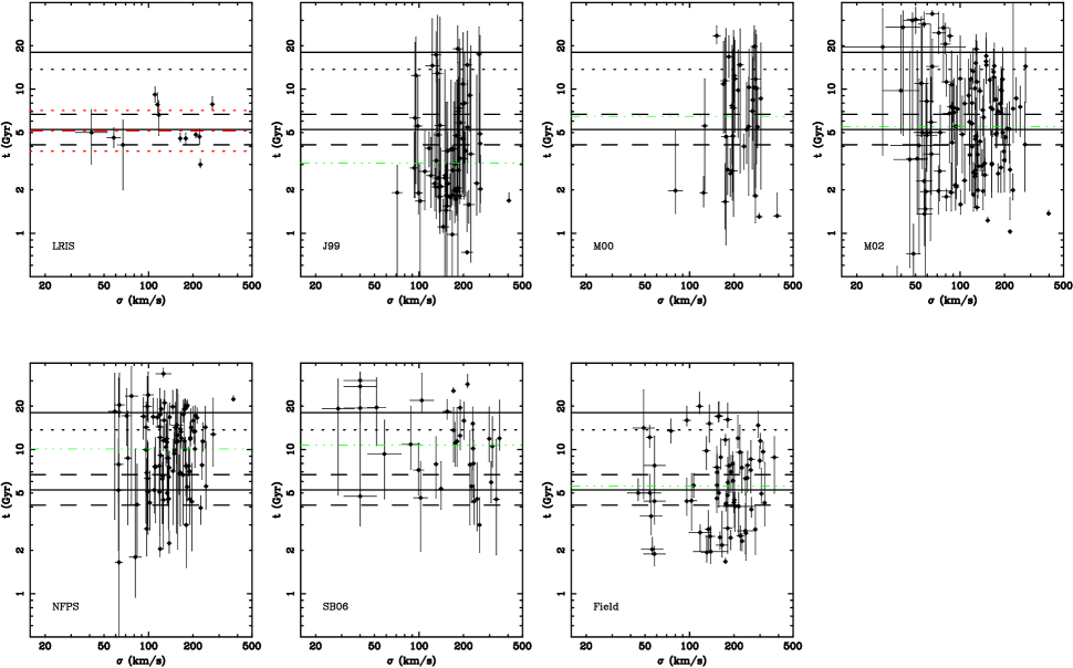
Figure 7: The $\log\sigma$–$\log t$ distributions for all Coma Cluster ETG and RSG samples. Top row, from left to right: the LRIS ETG sample; the Jørgensen (1999) ETG sample; the Mehlert et al. (2000) ETG sample and the Moore et al. (2002) ETG sample. Bottom row, from left to right: the Nelan et al. (2005) RSG sample (Coma Cluster galaxies only); the Sánchez-Blázquez et al. (2006b) ETG sample (Coma Cluster galaxies only); and our field sample of ETGs. The solid lines in all panels represent the mean age of the Coma Cluster ETGs after removing the two outliers GMP 3269 and GMP 3639, and the dashed lines represent the maximum internal scatter in age permitted by the data. The (red) dashed-dotted line in the LRIS panel is the mean age of the ETGs including the outliers, and the (red) dotted lines are the maximum scatter permitted by all twelve galaxies. The (green) dot-dashed line in each other panel is the (biweight) mean age of the sample. Note that many field ETGs are significantly older than the Coma Cluster ETGs at all velocity dispersions; this in itself is not a contradiction with prediction (ii) if the scatter in the field galaxies is larger at all velocity dispersion than in clusters. The upper dotted line is the current age of the Universe (13.7 Gyr, Spergel et al., 2007) and the upper solid line is the maximum age of the W94 models (18 Gyr).

In order to test this single age hypothesis, we have performed a Monte Carlo analysis in which we assume a single age for all of the galaxies in each sample but allow each galaxy in the sample to have its measured metallicity and enhancement ratio. We use our models to predict its line strengths and then perturb these using the observed errors (assuming a normal distribution). We then measure its predicted stellar population parameters. We do this in total one hundred times for each sample for each assumed age, in steps of $\Delta\log t=0.1$ dex from 0.1–1.2 dex (1.26–15.8 Gyr). At each age, we use a Kolmogorov-Smirnov (K-S) test to determine whether the age (and metallicity and enhancement ratio) distributions of the observed and simulated galaxies are drawn from the same parent distribution (similar to the approach of Moore, 2001). We compute the K-S probability $P_{\mathrm{KS}}$ for each of the 100 realisations at each age and take the average of the central 68 per cent of the $P_{\mathrm{KS}}$ distribution; we take the extremes of this central part of the distribution as the confidence limits. We assume that the null hypothesis, that the two populations are drawn from the same parent distribution, is strongly ruled out when $P_{\mathrm{KS}}\leq 0.05$ and marginally ruled out when $0.05<P_{\mathrm{KS}}\leq 0.10$; otherwise we assume that the null hypothesis is valid. Table 6 shows the results of these tests, and Figure 7 plots the ages as a function of $\log\sigma$. The results are as follows:

• Our LRIS sample is completely consistent with a constant age of $\log t=0.7$ dex and marginally consistent (within the confidence limits of the K-S probability distribution) with a constant age of $\log t=0.8$ dex; other mean ages are strongly ruled out.

• The Jørgensen (1999) sample is completely consistent with a constant age of $\log t=0.5$ dex and consistent with a constant age of $\log t=0.4$ dex.

• The Mehlert et al. (2000) sample is completely consistent with constant ages of $\log t=0.7$, $0.8$, and $0.9$ dex and marginally consistent with a constant age of $\log t=1.0$ dex (an age of $\log t=0.6$ is just on the edge of marginal acceptance).

• The Moore et al. (2002) sample is marginally consistent with a constant age of $\log t=0.6$ dex. This is in agreement with the findings of Moore (2001), who found that the Moore et al. (2002) ETG sample was inconsistent with a constant age when considering the the ellipticals and S0’s taken together; taken separately, however, the ellipticals and S0’s were each consistent with a different constant age. We have tested this hypothesis and find that both the elliptical and S0 galaxies in Moore et al. (2002) are consistent with constant ages of $\log t=0.7$ or 0.8 dex, and the ellipticals are marginally consistent with a constant age of $\log t=0.9$ dex. The K-S probabilities suggest that the S0’s are slightly younger (higher probability at $\log t=0.7$ dex than at 0.8 dex) than the ellipticals (higher probability at $\log t=0.8$ dex than at 0.7 dex). Note however that we have ignored transition morphologies such as E/S0, S0/E, and S0/a, as well as a few later-type galaxies in these tests.

• The Nelan et al. (2005) sample is at best marginally consistent with a constant age of $\log t=1.0$ dex.

• The Sánchez-Blázquez et al. (2006b) sample is consistent with constant ages of $\log t=1.0$ and $1.1$ dex and marginally consistent with with constant ages of $\log t=0.9$ and $1.2$ dex. This mean age deviates from all other Coma ETG samples. We return to this point in §5.2 below.

• Finally, our field sample is marginally consistent with a constant age of $\log t=0.7$ dex, but only at the extreme end of the 68 per cent confidence interval (as expected from Paper II). The average age of this sample is $\mu_{\log t}=0.70\pm 0.01$ dex ($5.0\pm 0.1$ Gyr), with a sizable scatter of 0.29 dex (3.3 Gyr) rms. This is identical within the formal errors to the mean age of the LRIS galaxies.

We have examined the ages of our field sample (§2.4) in order to understand our result in the context of prediction (ii), that ETGs in high-density environments should be older than those in low-density environments. The SSP-equivalent ages of the Coma Cluster and field ETGs and the typical ages and intrinsic age scatter of the Coma Cluster ETGs are shown as a function of velocity dispersion in Figure 7. This then is our first major result: Coma ETGs (in our small but extremely high-quality sample) are (i) (nearly) coeval in their SSP-equivalent ages and (ii) are identical in age to the field ETGs. In terms of our predictions, Coma ETGs appear to violate predictions (i), that lower-mass ETGs have younger stellar populations that high-mass ETGs, and (ii), that ETGs in high-density environments are older than those in low-density environments.

Figure 8: The estimated intrinsic logarithmic scatter as a function of velocity dispersion ($\sigma$) in the Coma Cluster ETG sample of Moore et al. (2002, solid squares) and our field galaxy sample (see text; open circles). Galaxies were binned in $\log\sigma$ such that each bin had an equal number of galaxies in the Moore et al. (2002) sample (12 galaxies per bin), except the bin with the highest $\sigma$, which had only two galaxies. Ignoring this bin, it is clear that the intrinsic age scatter in this sample increases with decreasing velocity dispersion. The field sample was binned into the same bins in $\sigma$ as the Coma sample, and the point size of each bin represents the number of field galaxies in that bin. It is important to remember that the field sample is not complete and is particularly missing galaxies at $\sigma<100\,\mathrm{km\,s^{-1}}$, and some bins are completely empty. Even so, it appears that the intrinsic age scatter in the field galaxies at high $\sigma$ is typically slightly higher than that of the Coma galaxies.

Our LRIS sample is too small to determine the age scatter as a function of mass, so it is difficult to say whether prediction (iii), that high-mass ETGs have a smaller age spread than low-mass ETGs, is violated or not; all we can say is that the intrinsic in our entire sample is small. However, the Moore et al. (2002) sample is large enough to make this test, as it contains 121 galaxies with usable stellar population parameters. We have binned these galaxies in velocity dispersion and determined the intrinsic scatter as described above; the results are plotted in Fig. 8. It is clear that the internal scatter tends to increase with decreasing velocity dispersion (except in the highest velocity dispersion bin, where only two galaxies contribute). Such an increase in the scatter in stellar population age with decreasing velocity dispersion has been reported previously by Poggianti et al. (2001), although their data were not as high quality as that of Moore et al. (2002, see Appendix B). We therefore suggest that the stellar populations of ETGs in the Coma Cluster are consistent with prediction (iii), in agreement with previous results. We find additionally that the field sample, at least for $\sigma>100\,\mathrm{km\,s^{-1}}$, where this sample may be representative (if not complete) has typically a slightly larger intrinsic age scatter at a given velocity dispersion. This further supports prediction (iii), but the difference is not large.

4.2.1 Caveats on stellar population ages

We have considered the possibility that our line strengths may be systematically too high in $\mathrm{H}\beta$, $\mathrm{Mg}\,b$, Fe5270, and Fe5335. We tested the effects on the inferred stellar population parameters of offsets of $\Delta\mathrm{H}\beta=-0.056$ Å, $\Delta\mathrm{Mg}\,b=-0.139$ Å, $\Delta\mathrm{Fe5270}=-0.090$ Å, and $\Delta\mathrm{Fe5335}=-0.091$ Å – the root-mean-square deviations of calibrations onto the Lick/IDS system (Table 11). These are the maximum allowable systematic shifts we can reasonably apply to our data, and are larger than the average differences with respect to other measurements in the literature (Table 12), except for Fe5335. We find that our LRIS galaxies are older by $\Delta\log t=0.16\pm 0.02$ dex and more metal-poor by $\Delta\mathrm{[Z/H]}=-0.12\pm 0.02$ dex (with negligible change in $\mathrm{[E/Fe]}$). This age shift translates into a mean age for the entire LRIS sample of $\mu_{\log t}=0.88\pm 0.02$ dex ($7.5\pm 0.3$ Gyr). If we require an average age of 10 Gyr for this sample, an offset of $\Delta\mathrm{H}\beta=-0.2$ Å (with no other index changes) is required for each galaxy, or nearly four times the Lick/IDS calibration uncertainties. We believe that this large shift is unlikely, and we can therefore accept a maximum average age of roughly 7–8 Gyr for this sample.

As mentioned in §2.3 above, we have not applied corrections for emission-line fill-in of $\mathrm{H}\beta$ in our LRIS line strengths. We warn the reader that this means that our age estimates are upper limits. Normal weak-lined red-sequence ellipticals are nearly always LINERS, in which case we expect $\mathrm{EW(\mathrm{H}\beta)}=0.62\times\mathrm{EW([O\,\textsc{iii}])}$ on average, with little scatter (e.g., Ho, Filippenko, & Sargent, 1997; Trager et al., 2000a; Yan et al., 2006). Therefore our detection of [Oiii] emission in most of our sample means that undetected $\mathrm{H}\beta$ emission is filling in our $\mathrm{H}\beta$ absorption lines in those galaxies, making them appear older than they truly are. We have made a simple attempt to make such a correction for fill-in using the correction quoted above and find that the mean age of our twelve galaxies is $\mu_{\log t}=0.618\pm 0.018$ dex ($4.1\pm 0.1$ Gyr). This is younger than that inferred above, as expected. This would actually make the Coma ETGs younger than the field ETGs, seriously violating prediction (ii).

Stellar population model differences can also affect the determination of stellar population parameters. The standard deviation of mean ages for the vanilla W94, Padova W94, and BC03 models modified as described in §3.2 is 28 per cent for the current sample, in the sense that the Padova W94 models give younger ages ($\langle\log t\rangle=0.59\pm 0.01$) than the vanilla W94 models ($\langle\log t\rangle=0.71\pm 0.02$), which in turn give younger ages than the BC03 models ($\langle\log t\rangle=0.81\pm 0.01$). Comparison of Figures 4 and 5 shows that the ages from the vanilla W94 models and TMB03 should in principle be very similar. Further, as discussed in §3.1, it possible that our models may be underestimating ages by as much as $\Delta\log t=0.25$ dex for $\log t\ga 0.6$ dex due to incorrect treatment of abundance ratio effects (Proctor & Sansom, 2002), but the true magnitude of this correction awaits the next generation of stellar population models.

Calibration, emission fill-in correction, and model differences may drive differences in the absolute stellar population parameters, but as shown by many previous studies (e.g., Paper I), relative stellar population parameters are nearly insensitive to changes in the overall calibration, emission corrections, or stellar population model. We therefore believe that the uniformity of ages of our Coma ETG sample and their similarity in ages when compared with field ETGs are robust results.

4.3 Correlations of stellar population parameters with each other and with velocity dispersion and mass

We now ask whether there are trends in the stellar population parameters as a function of other stellar population parameters or with other parameters such as velocity dispersion or mass. The latter correlations – if they exist – are relevant to prediction (i), the downsizing of the stellar populations of ETGs.

4.3.1 The $Z$-plane and the $\mathrm{[E/Fe]}$–$\sigma$ relation

Table 7: $Z$-plane and $\mathrm{[E/Fe]}$–$\sigma$ relation parameters for ETGs through an aperture of 2$\aas@@fstack{\prime\prime}$7 projected to the distance of the Coma Cluster, using new W94 models

	$\alpha$	$\beta$	$\gamma$, Zero-point	$\delta$	$\epsilon$, Zero-point
Data set	$d\mathrm{[Z/H]}/d\log\sigma$	$d\mathrm{[Z/H]}/d\log t$	($Z$-plane)	$d\mathrm{[E/Fe]}/d\log\sigma$	($\mathrm{[E/Fe]}$–$\sigma$)
Low-density environment ETG samples:
Paper IIa	$0.76\pm 0.13$	$-0.73\pm 0.06$	$-0.87\pm 0.30$	$0.33\pm 0.01$	$-0.58\pm 0.01$
Paper IIb	$1.05\pm 0.06$	$-0.71\pm 0.05$	$-1.51\pm 0.15$	$0.25\pm 0.02$	$-0.41\pm 0.01$
Fieldc	$1.19\pm 0.07$	$-0.72\pm 0.05$	$-1.85\pm 0.17$	$0.24\pm 0.01$	$-0.40\pm 0.01$
Coma Cluster ETG and RSG samples:
LRIS	$0.97\pm 0.12$	$-0.78\pm 0.12$	$-1.26\pm 0.31$	$0.35\pm 0.03$	$-0.64\pm 0.01$
Jørgensen (1999)	$1.38\pm 0.21$	$-0.94\pm 0.07$	$-2.09\pm 0.46$	$0.30\pm 0.04$	$-0.51\pm 0.01$
Mehlert et al. (2000)	$1.39\pm 0.31$	$-0.79\pm 0.08$	$-2.34\pm 0.78$	$0.32\pm 0.07$	$-0.57\pm 0.01$
Moore et al. (2002)	$1.12\pm 0.09$	$-0.81\pm 0.04$	$-1.58\pm 0.19$	$0.33\pm 0.02$	$-0.56\pm 0.01$
Sánchez-Blázquez et al. (2006b)d	$0.94\pm 0.12$	$-0.88\pm 0.12$	$-1.14\pm 0.34$	$0.21\pm 0.04$	$-0.36\pm 0.01$
Nelan et al. (2005)d	$1.23\pm 0.14$	$-0.96\pm 0.08$	$-1.80\pm 0.28$	$0.31\pm 0.02$	$-0.56\pm 0.01$

^aAs published in Paper II. These parameters were not measured from indexes projected to Coma distance but those in $r_{e}/8$-diameter aperture and were also inferred from original vanilla W94 models using the Tripicco & Bell (1995) non-solar abundance index response functions.

^bUsing vanilla W94 models with new non-solar abundance index response functions, as described in the text.

^cGalaxies from González (1993), Kuntschner (2000), and Fisher et al. (1996), excluding Virgo Cluster galaxies to simulate a ‘low-density environment’ sample, as described in §2.4.

^dComa Cluster galaxies only.

The stellar population parameters $\log t$, $\mathrm{[Z/H]}$, and $\mathrm{[E/Fe]}$ together with the velocity dispersion $\log\sigma$ form a two-dimensional family in these four variables, as shown in Paper II for elliptical galaxies in environments of lower density than Coma (including the Virgo and Fornax clusters). The correlation between age and velocity dispersion in that sample was weak and therefore we associated the two primary variables in the four-dimensional space with age and velocity dispersion in Paper II. This association is tantamount to declaring that there exists a temporal relation between SSP-equivalent age and metallicity and also that velocity dispersion plays a role in the formation of ETGs. We also associate age and velocity dispersion with the primary variables in this set of galaxies, as we find no correlation between age and velocity dispersion in the present sample. As in Paper II, we find at best a weak anti-correlation between $\log t$ and $\mathrm{[E/Fe]}$ (correlation coefficient of $-0.51$ for the LRIS sample), so we claim again that the variation in stellar population parameters can be split into an $\mathrm{[E/Fe]}$–$\sigma$ relation and a metallicity hyperplane, the $Z$-plane. The $Z$-plane has the form

$$\mathrm{[Z/H]}=\alpha\log\sigma+\beta\log t+\gamma$$ (3)

Coefficients of Eq. 3 are given in the first three columns of Table 7 for the original sample of Paper II using the models described therein; the sample of Paper II using the current vanilla W94 models; a sample consisting of local field E and S0’s from González (1993), Fisher et al. (1996), and Kuntschner (2000), removing the Virgo Cluster galaxies; the LRIS sample; and five other samples of Coma Cluster galaxies: Jørgensen (1999), Mehlert et al. (2000), Moore et al. (2002), Nelan et al. (2005, Coma Cluster galaxies only), and Sánchez-Blázquez et al. (2006b, Coma Cluster galaxies only). Coefficients were determined by minimising the minimum absolute deviations from a plane (after subtracting the mean values of each quantity), as described in Jorgensen et al. (1996) and used in Paper II. Uncertainties were determined by making 1000 Monte Carlo realisations in which the the line strength indexes of the galaxies were perturbed using their (Gaussian) errors, stellar population parameters were determined from the new indexes, and new planes were fit to these parameters. We find from these realisations that the slopes $\alpha$ ($=d\mathrm{[Z/H]}/d\log\sigma$) and $\beta$ ($=d\mathrm{[Z/H]}/d\log t$) are nearly uncorrelated with each other, but the zero-point $\gamma$ is strongly correlated with $\alpha$ and somewhat less with $\beta$.

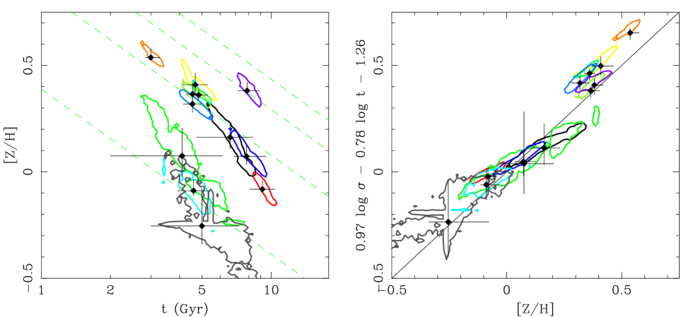
Figure 9: Two views of the $Z$-plane (Paper II) for the LRIS galaxies. Left: the $\log t$–$\mathrm{[Z/H]}$ projection (roughly face-on). Contours are 68 per cent confidence intervals of the stellar population parameters, marginalised over $\mathrm{[E/Fe]}$. The solid lines are lines of constant velocity dispersion $\sigma$ (from bottom to top: 50, 150, 250, 350 $\mathrm{km\,s^{-1}}$). Right: the (long-) edge-on projection, showing the thinness of the plane.

Figure 9 shows a roughly face-on view of the $Z$-plane – the $\log t$–$\mathrm{[Z/H]}$ projection – and the long edge-on view. The face-on view shows that there exists an age–metallicity relation for each value of $\sigma$, as shown in Paper II. We have argued in Paper II that the age–metallicity relation at fixed $\sigma$ in field samples is not a result of correlated errors in the age–metallicity plane, as the variations in ages and metallicities are many times larger than the (correlated) errors (see, e.g., right panel of Fig. 17 below). It is possible that correlated errors may bias the slope of the plane, but the existence of the plane is not driven by the correlated errors. In the current dataset, this age–metallicity relation is not strong, as the dispersion in age is very small for these galaxies, as shown above. The existence of an age–metallicity relation at fixed $\sigma$ with a slope $d\mathrm{[Z/H]}/d\log t\sim-2/3$ means that (optical) colours and metal-line strengths should be nearly constant at a given velocity dispersion, following the ‘Worthey 3/2 rule’ (Worthey, 1994). This results in thin Mg–$\sigma$ (as show in Paper II) and colour–magnitude relations. The thinness of the $Z$-plane (that is, the scatter perpendicular to the plane) suggests that age and velocity dispersion ‘conspire’ to preserve the thinness of such relations, which are nearly – but not quite (Paper II; Thomas et al., 2005; Gallazzi et al., 2006) – edge-on projections of the $Z$-plane.

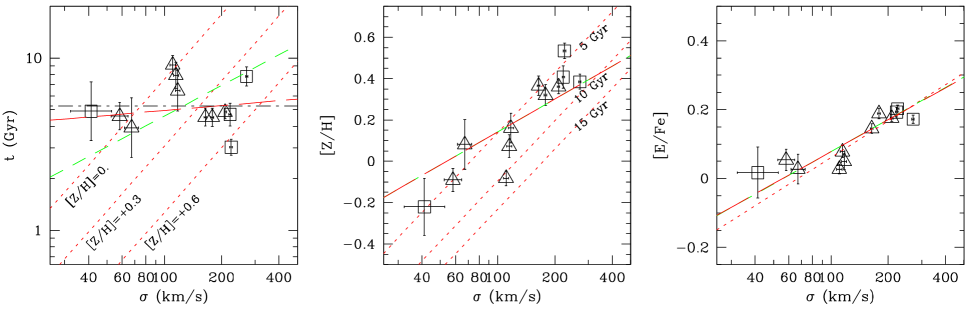
Figure 10: Correlations of stellar population parameters with velocity dispersion $\sigma$. From left to right: $\log\sigma$–$\log t$; $\log\sigma$–$\mathrm{[Z/H]}$; $\log\sigma$–$\mathrm{[E/Fe]}$. In all panels, green short-dashed lines are the inferred $\log\sigma$–stellar population parameter relations of Nelan et al. (2005), zero-pointed to the LRIS stellar population parameters, and red long-dashed lines are those inferred from the LRIS index strengths following the precepts of Nelan et al. (2005). In the left panel, the red dotted lines are the predictions of the $Z$-plane for populations with $\mathrm{[Z/H]}=0$, $+0.3$ (close to the mean metallicity of this sample), and $+0.6$. In the middle panel, the three red dotted lines are the predictions of the $Z$-plane for populations of 5, 10, and 15 Gyr from top to bottom.

In Figure 10 we plot the stellar population parameters as a function of the velocity dispersion, which are just projections of the $Z$-plane and the $\mathrm{[E/Fe]}$–$\sigma$ relation. We find both a strong $\log\sigma$–$\mathrm{[Z/H]}$ relation (with a correlation coefficient of $0.91$; middle panel of Fig. 10) and a strong $\log\sigma$–$\mathrm{[E/Fe]}$ relation (with a correlation coefficient of $0.88$; right panel of Fig. 10), but we see no $\log\sigma$–$\log t$ correlation (correlation coefficient of $0.01$; left panel of 10), as expected from our discussion in §4.2. The latter result is again in contradiction of our prediction (i) for the stellar populations of ETGs, suggesting that there is apparently no downsizing in Coma Cluster ETGs.

The $\log\sigma$–$\mathrm{[Z/H]}$ correlation is just the mass–metallicity relation for ETGs (Faber, 1973, 1977). The distribution of galaxies in the face-on ($\log t$–$\mathrm{[Z/H]}$) projection of the $Z$-plane (left panel of Fig. 9) makes it clear why a strong mass–metallicity relation exists for the LRIS sample of Coma Cluster galaxies: the galaxies have nearly a single age, so the dispersion in metallicity $\mathrm{[Z/H]}$ translates into a velocity dispersion–metallicity sequence (which is related to a mass–metallicity relation through the virial relation $M\propto\sigma^{2}r_{e}$). This can be seen from the $\log\sigma$–$\mathrm{[Z/H]}$ relations predicted from the $Z$-plane (dotted line in the middle panel of Fig. 10). This is not the case in samples that have large dispersions in age, like that of Paper II, because galaxies in these samples have anti-correlated age and metallicity at fixed velocity dispersion, which erases the observed mass–metallicity relation. That there is such a strong velocity dispersion–metallicity relation in the LRIS sample is further evidence that there is at best a weak velocity dispersion–age relation.

The $\log\sigma$–$\mathrm{[E/Fe]}$ correlation was discovered by Worthey et al. (1992) and called the $\mathrm{[E/Fe]}$–$\sigma$ relation by Paper II, who found a relation of the form

$$\mathrm{[E/Fe]}=\delta\log\sigma+\epsilon.$$ (4)

The last two columns of Table 7 give the coefficients of Eq. 4 for the samples considered here. A slope of $\alpha=0.41$ is found for the LRIS galaxies. This value is roughly consistent with the relations given by Paper II and Thomas et al. (2005), which were based on models with different prescriptions for correcting line strengths for $\mathrm{[E/Fe]}$. We note that the right panels of Figures 6 and 10 suggest that the distribution of $\mathrm{[E/Fe]}$ in the LRIS sample may be bimodal, but this is likely to be an effect of the small sample size.

We discuss the origin of both of the $Z$-plane and $\mathrm{[E/Fe]}$–$\sigma$ relation in §5.4.

4.3.2 Velocity dispersion– and mass–stellar population correlations

In Figure 7 we show the distributions of $\log t$ as a function of $\log\sigma$ for all of the Coma Cluster samples at our disposal. We have fit linear relations to these parameters (not shown) using the routine FITEXY from Press et al. (1992), which takes into account errors in both dimensions. In all samples except the Nelan et al. (2005) RSG sample, we find negative correlations between age and velocity dispersion, violating prediction (i) for the ages of ETGs in Coma.

Unfortunately, it is difficult to determine the slopes of relations such as $\log\sigma$–$\log t$ for samples with large scatter in the stellar population parameters from directly fitting the results of grid inversion, either due to intrinsic scatter or just very uncertain measurements. We have therefore also implemented two other methods for determining the slopes of $\log\sigma$–, $\log M_{*}$–, and $\log M_{\mathrm{dyn}}$–stellar population parameter relations. The first is the ‘differential’ method described by Nelan et al. (2005). The second (‘grid inversion’) method is very similar to the ‘Monte Carlo’ method of Thomas et al. (2005), although our implementation is somewhat different: (a) we use a full non-linear least-squares $\chi^{2}$-minimisation routine (Thomas et al. fit ‘by eye’); (b) we do not attempt to account for extra scatter in the relations; and (c) we do not attempt to fit two-component (old plus young) population models to outliers. Our inferred slopes for the Thomas et al. (2005) high-density sample match their results closely, giving us confidence that our method is at least similar to theirs. We find no significant positive $\sigma$– or mass–age relation for any Coma Cluster ETG sample in either method. Only the Nelan et al. (2005) RSG sample has a significantly ($>2\sigma$) positive slope in this relation.

These relations imply three important results. (1) RSGs in nearby clusters – here represented by the Nelan et al. (2005) samples, including the Coma Cluster itself – have a strong age–$\sigma$ relation, such that low-$\sigma$ or low-mass galaxies have younger ages than high-$\sigma$ or high-mass galaxies, as pointed out by Nelan et al. (2005). (2) Taken together, samples of ETGs in the Coma Cluster show no significant age–$\sigma$ or age–mass relation. (3) ETGs in the field show an age–$\sigma$ relation as strong as the Coma Cluster RSG sample of Nelan et al. (2005). Results (1) and (2) are apparently contradictory – why should RSGs show a strong age–$\sigma$ relation while ETGs show no such relation? In advance of a full discussion in §5.3, a difference in emission-line corrections between the Nelan et al. (2005) RSG sample and the ETGs sample is likely to be the cause, not a real age–$\sigma$ relation in the RSGs. We are therefore again faced with the conclusion that prediction (i), the downsizing of the stellar population ages of ETGs, is apparently violated in the Coma Cluster.

5 Discussion

In §1 we made three predictions for the stellar populations of ETGs – early-type galaxies, galaxies morphologically classified as elliptical or S0 – in high-density environments: (i) low-mass ETGs in all environments are younger than high-mass ETGs (a prediction that we have called downsizing in this work); (ii) ETGs in high-density environments are older than those in low-density environments; and (iii) massive ETGs in high-density environments have a smaller spread in stellar population age than lower-mass ETGs and those in lower-density environments. We recall that our predictions are based on associating ETGs – early-type galaxies, galaxies selected to have elliptical and S0 morphologies – with RSGs – red-sequence galaxies, galaxies selected by colour to be on the red sequence – and using the results of high-redshift observations and the predictions of semi-analytic models of galaxy formation.

We found in §4 that ETGs in the Coma Cluster have a mean age of 5–7 Gyrs (including line-strength index calibration uncertainties but not model uncertainties) and appear to be drawn from a single-aged population. Further, the age scatter decreases with increasing mass. Finally, while we do find a $Z$-plane for Coma Cluster ETGs and RSGs, we find no evidence of an age–$\sigma$ or age–mass relation for the ETGs. Therefore ETGs in the Coma Cluster appear to follow prediction (iii) and (perhaps) prediction (ii) but violate prediction (i). In this section, we discuss first what we mean by ‘age’ for old stellar populations, then discuss why we appear to disagree with previous studies that found downsizing in high-density environments, what the mean SSP-equivalent age of the Coma Cluster ETGs implies for their formation, and finally speculate about the origin of the $Z$-plane, and mass–metallicity and $\mathrm{[E/Fe]}$–$\sigma$ relations.

5.1 What are we measuring?

A worry with stellar population analysis of non-star-forming galaxies based on their Balmer-line strengths has long been that these lines reflect not younger (intermediate-aged) main-sequence turn-off stars but some other hot population, such as blue stragglers (e.g., Rose, 1985, 1994, Paper I) or blue horizontal branch stars (e.g., Burstein et al. 1984; Paper I; Maraston & Thomas, 2000; Trager et al., 2005, and references therein). Such populations have Balmer-line strengths comparable or stronger than intermediate-aged main-sequence turn-off stars and should significantly alter the observed ‘ages’ if present in large enough (in luminosity-weighted terms) numbers. Trager et al. (2005) showed in detail that blue horizontal-branch stars actually affect inferred metallicities more than ages, based on observations of blue absorption lines in the present sample. Intermediate-aged populations are therefore still required for the LRIS sample. Thus we believe that our age estimates are not affected by hot blue stars that are not intermediate-aged main-sequence turn-off stars.

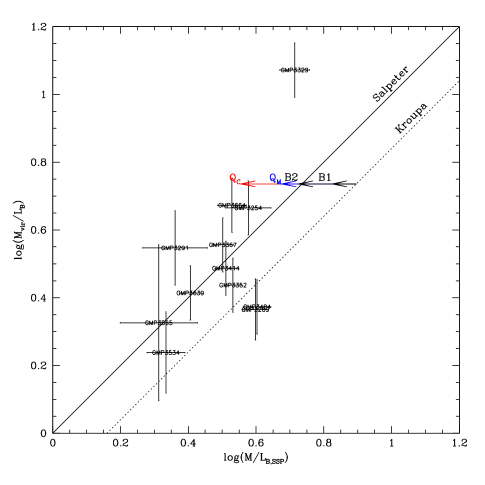
Figure 11: The virial mass-to-light ratios in the $B$-band of our LRIS sample ETGs as a function of the stellar mass-to-light ratios as determined from the best-fitting SSP models. The W94 models are computed using a Salpeter (1955) IMF, represented by the solid (one-to-one) line. Using the Kroupa (2001) IMF decreases the SSP model mass-to-light ratios by $\sim 30$ per cent ($\Delta\log(M/L)\sim-0.16$, Cappellari et al., 2006), as shown by the dotted line. The arrows represent the effect of different star formation histories on the mass-to-light ratios: B1 and B2 are bursts occurring 1 and 2 Gyr ago on top of a 12.3 Gyr-old population, resulting in $t_{S}SP=5$ Gyr; Q_c and Q_m are quenching models with the same $t_{S}SP=5$ Gyr. All of the arrows have the same starting location and so have lengths $\mathrm{Q}_{c}>\mathrm{Q}_{m}>\mathrm{B}1>\mathrm{B}2$. We note that if all the galaxies have a Kroupa IMF and also contain 30 per cent of their mass in dark matter within the 2$\aas@@fstack{\prime\prime}$7 aperture used to measure the line-strengths, they should lie on the Salpeter IMF line.

However, it must always be remembered that the ages, metallicities, and enhancement ratios we measure with our methods are SSP-equivalent parameters. We first ask if it is possible that the galaxies can in fact be the single stellar populations we have assumed in our modelling. A simple test of this model is to ask whether we can reproduce the virial mass-to-light ratios derived in §2.5 using SSP models. We compare the inferred stellar $M/L$ ratios with the virial $M/L$ ratios in Figure 11. Three points can be gleaned from this figure: (a) the Salpeter (1955) IMF appears to be unphysical for these galaxies, given the presence of many galaxies to the right of the Salpeter IMF line. Therefore, as in Cappellari et al. (2006), we take a Kroupa (2001) IMF to be a better representation of the (low-mass star) IMF than the Salpeter IMF; (b) even assuming a small amount (30 per cent) of dark matter within the observed radius in each galaxy (Cappellari et al., 2006), most of the galaxies have SSP-equivalent stellar $M/L$ ratios too low for their virial $M/L$, suggesting that a complex star-formation history is required in these galaxies; and (c) quenching (arrow Q_c and Q_m) appears to be too extreme for most of the galaxies.

We have further examined the GALEX (Martin et al., 2005) photometry of galaxies in the LRIS sample as a probe of young, hot stars. Only three of our galaxies – GMP 3414, GMP 3565, and GMP3664 – have GALEX photometry publicly available in GR3. (Unfortunately, the bright star HD 112887 prevents GALEX from observing the are directly around the cD galaxy GMP 3329=NGC 4874.) Of these three, only GMP 3565 is ‘UV-strong’ in the notation of Yi et al. (2005) – $(FUV-r)<5$ and $(NUV-r)<4$ mag – indicating very young ($t\sim 0.1$ Gyr) stars. A total of five galaxies in all of the ETGs with line strengths considered in this study (from all sources) are in this ‘UV-strong’ class, and their $\mathrm{H}\beta$-strengths and ages are uncorrelated with their UV–optical colours. Using the more generous ‘young’ galaxy criterion of Kaviraj et al. (2007a) – $(NUV-r)<5.5$ mag – 51 galaxies in the total sample are ‘young’ (out of 109 with NUV photometry), although only 17 have $(NUV-r)<5$ mag and only eight (including GMP 3565 in the LRIS sample) lie significantly off of the $NUV-r$ ‘red sequence’. This may suggest that very young populations are not significantly contaminating our age estimates.

Clearly therefore the populations of ETGs are more complicated than single-burst populations (e.g. Ferreras & Yi, 2004; De Lucia et al., 2006). Serra & Trager (2007) have explored two-burst ‘frosting’ models and Trager & Somerville (in prep.) explore more complicated star-formation histories using semi-analytic galaxy formation models. Taken together these studies find that SSP-equivalent $\mathrm{[Z/H]}$ and $\mathrm{[E/Fe]}$ represent their luminosity-weighted quantities. SSP-equivalent age, however, represents a degenerate mixture of recent star-formation age and burst strength, as suggested in Paper II. Moreover young and intermediate-aged populations contribute much more to the age-sensitive line strengths than is suggested by the phrase ‘light-weighted’, because younger populations have much higher mass-to-light ratios in the Balmer lines than old populations. This is why small ‘frostings’ of recent star formation (Paper II; Gebhardt et al., 2003) or recent truncation of ‘quenching’ of previously-on-going star formation (e.g., Couch & Sharples, 1987; Bell et al., 2004b; Harker et al., 2006, and many others) lead to much younger SSP-equivalent ages.

As a simple example, a two-burst model with 98 per cent of the mass in an 12 Gyr-old population (a formation redshift of $z_{f}=4$) and the remaining 2 per cent of the mass in 1 Gyr population (a burst redshift of $z_{b}=0.08$) results in an SSP-equivalent age of 5 Gyr. Note that as the young population becomes older, much more mass is required: for a 2 Gyr old burst (a burst redshift of $z_{b}=0.16$), 12 per cent of the stellar mass needs to be in the younger population for this population to also have an age of 5 Gyr. The effect of these two-burst models on the stellar $M/L$ ratios are shown in Figure 11, clearly reducing the stellar $M/L$ ratios by the addition of much brighter, slightly more massive stars.

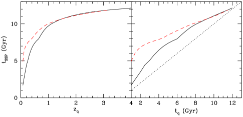
Figure 12: The relation between present-day SSP-equivalent age $t_{\mathrm{SSP}}$ and (left panel) quenching redshift $z_{q}$ and (right panel) quenching time $t_{q}$. In each panel, the solid line represents quenching models with constant star formation from $z=5$ to $z_{q}$, while the (red) dashed line represents quenching models with star formation that follows the ‘Madau plot’ (as parametrised by Hopkins & Beacom, 2006, see text). The dashed line in the right panel is equivalence between $t_{\mathrm{SSP}}$ and $t_{q}$.

Table 8: SSP-equivalent, mass-weighted, and $B$-band light-weighted ages of quenched galaxies

$t_{q}$		$t^{c}_{\mathrm{SSP}}$	$t^{c}_{M}$	$t^{c}_{B}$	$t^{m}_{\mathrm{SSP}}$	$t^{m}_{M}$	$t^{m}_{B}$
(Gyr)	$z_{q}$	(Gyr)	(Gyr)	(Gyr)	(Gyr)	(Gyr)	(Gyr)
1.0	0.075	1.84	4.60	3.33	5.23	8.41	7.32
1.5	0.116	2.60	5.22	3.90	6.21	8.48	7.48
2.0	0.160	3.50	5.74	4.57	6.83	8.56	7.68
2.5	0.206	4.45	6.21	5.19	7.20	8.65	7.89
3.0	0.256	5.04	6.65	5.77	7.47	8.75	8.09
3.5	0.308	5.81	7.05	6.32	7.68	8.85	8.30
4.0	0.365	6.45	7.43	6.82	7.87	8.97	8.50
4.5	0.427	6.97	7.79	7.28	8.09	9.09	8.69
5.0	0.493	7.37	8.14	7.71	8.44	9.22	8.88
5.5	0.566	7.69	8.48	8.11	8.75	9.36	9.07
6.0	0.646	7.98	8.80	8.50	9.05	9.51	9.27
6.5	0.735	8.56	9.12	8.86	9.34	9.66	9.46
7.0	0.833	9.09	9.43	9.21	9.63	9.83	9.66
7.5	0.945	9.55	9.72	9.55	9.88	10.00	9.86
8.0	1.072	9.92	10.02	9.88	10.11	10.18	10.07
8.5	1.218	10.23	10.30	10.20	10.32	10.37	10.29
9.0	1.390	10.53	10.58	10.51	10.53	10.57	10.51
9.5	1.596	10.81	10.86	10.80	10.75	10.78	10.74
10.0	1.848	11.09	11.13	11.09	10.99	11.01	10.98
10.5	2.166	11.36	11.39	11.37	11.24	11.26	11.24
11.0	2.587	11.63	11.65	11.64	11.52	11.53	11.52
11.5	3.174	11.88	11.91	11.91	11.81	11.83	11.83

Model galaxies are assumed to begin star formation at $z=5$ (lookback time of 12.3 Gyr). Columns.– (1) Quenching time. (2) Quenching redshift. (3) Present-day SSP-equivalent age of composite stellar population for constant star formation model ($c$). (4) Present-day mass-weighted age of composite stellar population for constant star formation model. (5) Present-day $B$-band light-weighted age of composite stellar population for constant star formation model. (6)–(9) As in columns (4)–(6) for Madau-curve model ($m$). See text for details.

As slightly more complex examples, we construct two simple ‘quenching’ models. In this sort of model, a galaxy forms stars – perhaps with a constant star formation rate, or with a declining rate – until star formation is suddenly truncated (e.g., Bell et al., 2004b; Faber et al., 2007). We assume that a galaxy starts forming stars at $z=5$ (a lookback time of 12.3 Gyr in our assumed cosmology) and ceases forming stars at some ‘quenching redshift’ $z_{q}$ corresponding to a ‘quenching age’ (lookback time) of $t_{q}$. We then ask what its SSP-equivalent age $t_{\mathrm{SSP}}$ is today. In the first model, we assume that the galaxy forms stars at a constant rate from $z=5$ to $z_{q}$; this is model $c$ (for constant star formation), typical of the star-formation histories of Sc disc galaxies (Sandage, 1986; Kennicutt, 1998). In the second model, we assume that the galaxy forms stars at rate that follows the star formation history of the Universe – the ‘Madau plot’, after Madau et al. (1996) – as parametrised by Hopkins & Beacom (2006); this is model $m$ (for ‘Madau’), and is similar to the star-formation histories of early-type (Sa–Sb) spirals (Sandage, 1986; Kennicutt, 1998). In both models we assume star formation is stopped completely at $z_{q}$ with no associated burst. We further assume no chemical evolution; rather, we assume that $\mathrm{[Z/H]}=\mathrm{[E/Fe]}=0$ dex at all times (an unrealistic assumption!). The results are plotted in Figure 12 and tabulated in Table 8. We see that the SSP-equivalent age $t_{\mathrm{SSP}}$ is a good tracer of the quenching time $t_{q}$ or redshift $z_{q}$, although $t_{\mathrm{SSP}}\geq t_{q}$ at all ages in these models. This is due to the composite nature of $t_{\mathrm{SSP}}$, in which stars of all ages contribute to the age indicators (here $\mathrm{H}\beta$). However, in nearly all cases, $t_{\mathrm{SSP}}<t_{M,B}$, where $t_{M}$ and $t_{B}$ are the mass-weighted and $B$-band-luminosity-weighted ages, because the youngest populations contribute most to $t_{\mathrm{SSP}}$ due to their low mass-to-light (high light-to-mass) ratios. We show the effect of these models on the stellar $M/L$ ratios in Figure 11; model $c$ appears to be too extreme if dark matter is present within the observed apertures of these galaxies, but model $m$ is possibly consistent with the observed trend for most galaxies.

Figure 13: The deviation of rest-frame $U-B$ colour from a typical red sequence galaxy as a function of redshift $z$ for a 12.3 Gyr-old galaxy quenched at $z_{q}=0.25$, having formed stars at a constant rate before that. The red sequence galaxy is assumed to have formed 6.5 Gyr ago ($z_{f}=0.74$) and so has the same colour as the quenched galaxy at $z=0$. The dotted line at $\Delta(U-B)=-0.030$ is RMS dispersion of cluster red sequences from van Dokkum & Franx (2001) and the dashed line at $\Delta(U-B)=-0.036$ corresponds to the Butcher & Oemler (1984) division between red and blue galaxies at $\Delta(B-V)=-0.2$. Note that the colour difference becomes larger than both of these divisions at $z>0.09$.

These simple models point out that recent ‘quenching’ can produce significantly younger populations, as measured by the line strengths, than might be expected from a simple mass- or light-weighted estimate (cf. Harker et al., 2006). An advantage of quenching models is that relations like the mass–metallicity and the $\mathrm{[E/Fe]}$–$\sigma$ relation are generated naturally from the progenitors, which already possess these relations (§5.4 below). There is a problem with such simple quenching models, however. If the galaxies have continuous (if not constant) star formation before quenching, they are quite blue for a significant period after quenching. We compare the rest-frame $U-B$ colour evolution of a model $c$ galaxy quenched $z_{q}=0.2$ ($t_{q}=3$ Gyr) with an SSP galaxy with the same colour at $z=0$, which has $t_{\mathrm{SSP}}=6.5$, in Figure 13. We show also the typical scatter in rest-frame $U-B$ in the red sequences clusters at $z\la 0.8$, $\sigma_{U-B}\approx 0.03$ (van Dokkum & Franx, 2001), and the Butcher-Oemler colour division between red and blue galaxies, $\Delta(B-V)=-0.2$ (Butcher & Oemler, 1984), corresponding to $\Delta(U-B)=-0.036$ – strikingly similar to the typical scatter in the red sequence (as desired Butcher & Oemler, 1978). The simple quenching model remains a ‘blue’ Butcher-Oemler galaxy until as late as $z=0.09$, significantly below $z_{q}=0.25$ (a total time of 1.8 Gyr). Therefore, as suggested by van Dokkum & Franx (2001), quenched galaxies must continually join the red sequence at all redshifts to preserve the observed tight red sequences in clusters.

5.2 The mean age of Coma Cluster ETGs

In §4.2 we found a mean age of $\log t=0.72\pm 0.02$ dex, or $5.2\pm 0.2$ Gyr, for the high-precision and high-accuracy LRIS ETG sample, and that we could accept a mean age as old as 7.5 Gyr. Such a young mean age of the Coma Cluster ETGs – 5–7 Gyr, including calibration uncertainties – is surprising. We must ask whether we see other ‘young’ ETGs in other clusters at the same masses? We certainly see signs of recent star formation and accretion activity in massive galaxies at the centres of clusters: the young globular clusters in NGC 1275 (Pegasus A: see, e.g., Holtzman et al., 1992; Carlson et al., 1998); the multiple nuclei of NGC 6166 (the cD of Abell 2199: see, e.g., Minkowski, 1961; Tonry, 1984; Lauer, 1986) and indeed of many other cD galaxies, more than half of which are likely gravitationally bound (Tonry, 1985); and the depressed $\mathrm{Mg}_{2}$ and $D_{4000}$ indexes found in the central galaxies of cool-core clusters, indicative of recent star formation (Cardiel, Gorgas, & Aragon-Salamanca, 1995, 1998). These galaxies appear to have recently-formed stars accreted from smaller objects. On the other hand, the presence of young low-mass ETGs has been noted for some time (e.g., Rose, 1985, 1994; González, 1993; Trager et al., 1993, 2000b; Caldwell et al., 2003; Thomas et al., 2005; Nelan et al., 2005; Bernardi et al., 2006, just to name a few studies), and these galaxies may have formed their stars in situ (e.g., Thomas et al., 2005). But the striking result here is that the massive but not central ETGs in the Coma Cluster have (on average) young SSP-equivalent ages.

If we apply to the ‘quenching’ models described in §5.1 above, we find that model $c$, constant star formation followed by sudden quenching, predicts a quenching redshift of $z_{q}\approx 0.25$–0.43 (Table 8); model $m$ predicts a much more recent quenching epoch, $z_{q}\approx 0.08$–0.2. It appears from these models that Coma Cluster ETGs have recently been quenched by some process. For either model, such a recent quenching epoch suggests that the galaxies either just arrived on (model $c$) or should still be too blue for (model $m$) the red sequence, and that there will be no red sequence in the Coma Cluster at $z\ga 0.2$ if all of the ETGs quenched at the same, very recent time. We certainly do not see a large population of ‘young’ or blue ETGs in intermediate-redshift clusters, at least at moderate-to-high ETG masses, as judged from studies of the evolution of galaxy colours (e.g., Butcher & Oemler, 1978, 1984; Ellis et al., 1997; Stanford, Eisenhardt, & Dickinson, 1998), the Fundamental Plane (e.g., van Dokkum & Franx, 1996; van Dokkum et al., 1998, 1999; van der Wel et al., 2004; Treu et al., 2005), mass-to-light ratios (van der Marel & van Dokkum, 2007), and absorption-line strengths (Jørgensen et al., 2005; Kelson et al., 2006). The majority of the massive galaxies in intermediate-redshift clusters are quite red (e.g., Butcher & Oemler, 1978, 1984; Ellis et al., 1997; Yee et al., 2005), with very few, if any, blue galaxies among the bright ($L>2L_{\ast}$) population. We therefore consider such extreme quenching models ruled out.

If we adopt instead a two-burst model of star formation in Coma Cluster ETGs and assume an mean age of 5 Gyr, we require that 2 per cent of the mass (in our 2$\aas@@fstack{\prime\prime}$7 aperture) in each galaxy was formed at $z=0.08$ or 12 per cent of the mass at $z=0.16$, while the rest of the mass formed at $z_{f}=4$ (§5.1). This scenario allows for most of the mass to be formed at high redshifts while requiring only small bursts of recent star formation. Moreover, Yi et al. (2005) have shown that the FUV- and NUV-optical colours of massive early-type galaxies suggest that 15% of these objects have had recent star formation. Kaviraj et al. (2007b) have shown further that truly passive evolution of ETGs is in conflict with the evolution of their rest-frame UV-optical colours, such that 5–13 per cent of the entire mass in ETGs at $0.5<z<1$ resulted from star formation events less than 1 Gyr previous to the epoch of observation, although this number decreases by a factor of two by $z=0$. They suggest that massive ETGs have formed 10–15 per cent of their total mass since $z=1$, while low-mass ETGs have formed as much as 60 per cent of their mass in that time. We note however that their sample considered is a field sample, unlikely to contain a significant number of cluster galaxies.

Simplistically, in the two-burst case, we require that most ETGs in the Coma Cluster suffered an event that either triggered star formation simultaneously at redshifts in the range $z\sim 0.1$–0.2. This agrees well with the observation by Gerhard et al. (2007) that ‘perhaps 30 per cent’ of galaxies in the core Coma Cluster are involved in an on-going subcluster merger, suggesting that ‘Coma is forming now!’ (their emphasis). Our results support the view that the Coma Cluster is a very active region, with a large fraction of the ETGs within $r_{vir}/3$ having suffered star formation recently, at redshifts around $z\sim 0.1$–0.2. However, this scenario also requires there to be a significant population of blue galaxies at all masses in the Coma Cluster at those redshifts – which we have said above is unlikely, given the relatively tight red sequences in intermediate-redshift clusters.

There is also the possibility that we have been unlucky with our sample selection. The mean ages of the Sánchez-Blázquez et al. (2006b) Coma sample deviate from the other Coma ETG samples, as is clear from Table 6 (ignoring for present the red-sequence sample of Nelan et al. 2005). However we have found that the ages of four of the five galaxies in common (GMP 3254, 3269, 3639, and 3664) are the same within $1\sigma$, and the fifth, GMP 3329 (=NGC 4874), has a younger age but a higher metallicity from our data as a result of a higher $\mathrm{Mg}\,b$ – but nearly identical $\mathrm{H}\beta$ – strength in the LRIS data. It is notable that the four galaxies in common with the same ages in both samples are among the youngest in the Sánchez-Blázquez et al. (2006b) sample, and thus we may have been unlucky to select an unrepresentative sample of galaxies in the cluster. On the other hand, we note here that 20 per cent of the Sánchez-Blázquez et al. (2006b) sample (7/35 galaxies) have ages that are more than $1\sigma$ older than 14 Gyr – and therefore older than current estimates of the age of the Universe (Spergel et al., 2007) – using the vanilla W94 models. This suggests that the Sánchez-Blázquez et al. (2006b) galaxies may be on average too old, and that this is likely due to uncorrected emission. We therefore consider that their old mean age of 12.3 Gyr (after correcting for a reasonable amount of intrinsic scatter; the weighted mean without this correction is $>18\,\mathrm{Gyr}$, older than the oldest models and significantly older than the present age of the Universe) may be unreliable.

We are left with a conundrum: we either were very unlucky in our sample selection or we require Coma Cluster galaxies to form stars over an extended time in such a way as to ‘conspire’ to have the same $t_{\mathrm{SSP}}$ today but not produce too many blue galaxies at relatively recent lookback times. As we noted above, massive, central galaxies have young stars apparently acquired through accretion, while low-mass galaxies may have just shut down their internal star formation; perhaps these process have gone on independently and we have just chanced upon the right time to see them all have the same age. The increased scatter in the ages of low-mass Coma ETGs (Fig. 8) suggests that the process of shutting down star formation in the low-mass galaxies is an extended process, and we may have just gotten lucky in finding the ages well-synchronised.

Finally, we find a mean age of $\log t=0.70\pm 0.01$ dex, or $5.0\pm 0.1$ Gyr, for the field sample of González (1993), Fisher et al. (1996), and Kuntschner (2000), completely consistent with the age of the LRIS ETG sample, and consistent with the typical ages of nearly all of the Coma Cluster ETG samples (except Sánchez-Blázquez et al. 2006b; see Table 6). Thus, unlike Thomas et al. (2005), Bernardi et al. (2006) and Sánchez-Blázquez et al. (2006c), we find no significant difference between field and cluster ETGs, although this is strictly true only for the Coma Cluster.

5.3 Downsizing in the Coma Cluster or not?

One of our three robust predictions for the stellar populations of local RSGs – and by assumption, local ETGs – is that low-mass RSGs and ETGs are younger than high-mass RSGs and ETGs. In §1 we called this phenomenon downsizing by analogy with the decrease in specific star formation rate with decreasing redshift. In §4 we find no evidence of an age–mass or age–$\sigma$ relation at the $>1.5\sigma$ level (ignoring model variations) in any of the Coma Cluster ETG samples. However, we do find significant age–$\sigma$ and age–mass relations for the Nelan et al. (2005) Coma Cluster RSG sample and a significant age–$\sigma$ relation for the entire Nelan et al. (2005) cluster RSG sample and in the Thomas et al. (2005) high-density ETG sample.

5.3.1 Why does the Coma Cluster not show downsizing?

One possibility is that the Coma Cluster is somehow special, being a very rich cluster. In the Nelan et al. (2005) sample, it has the twelfth-highest cluster velocity dispersion and is the fifth most-X-ray-luminous cluster in the full sample, and it is the X-ray brightest and most massive cluster at $cz_{hel}<10000\,\mathrm{km\,s^{-1}}$. Because of its richness and velocity dispersion, it might be expected to contain old galaxies with little recent star formation. We have examined the age–$\sigma$ relations for both the full Nelan et al. (2005) sample, containing nearly 3500 RSGs (after removing galaxies contaminated by emission) in 93 clusters, and that sample restricted to just the Coma Cluster (97 RSGs). We find a significant age–$\sigma$ relation for both the full Nelan et al. (2005) sample – using the ‘differential’ method described by Nelan et al. (2005) and using the W94 models, we find $t\propto\sigma^{0.58\pm 0.15}$ – and for the restricted Coma Cluster sample – $t\propto\sigma^{0.39\pm 0.12}$. The relation for the Coma Cluster is only marginally shallower than that found for the entire Nelan et al. (2005) sample: a slope difference of $0.19\pm 0.19$. We suggest below that the significant age–$\sigma$ slope for the Nelan et al. (2005) Coma Cluster sample may be due to a lack of emission-line correction in the Balmer line strengths of that sample, which is also true for the entire sample. If the Coma Cluster RSGs truly possess an age–$\sigma$ relation, the results of Nelan et al. (2005) and our analysis suggest that its slope is cannot be much shallower than that of RSGs in typical high-density regions. This suggests that the lack of an age–$\sigma$ relation for the ETG samples is not due solely to the overall richness of the Coma Cluster.

Another possibility is that galaxies in the centre of the Coma Cluster are preferentially younger than the cluster as a whole. Studies of the diffuse light in the centre of the Coma Cluster (e.g., Thuan & Kormendy, 1977; Gregg & West, 1998; Adami et al., 2005a, a) and intracluster planetary nebulae (Gerhard et al., 2007) suggest that the centre of the Coma Cluster is a violent place, with a massive on-going merger of a subcluster (Gerhard et al., 2007). The Moore et al. (2002) sample however covers the inner $1^{\circ}$ of the cluster, which corresponds to a radius of $r_{vir}/3$ (Łokas & Mamon, 2003). We find no age–$\sigma$, age–$\log M_{*}$ nor age–$\log M_{\mathrm{dyn}}$ relation in this sample, and so a seriously different age of the centre – older or younger – is unlikely.

Finally, we note that we are not the first to find a flat age–$\sigma$ relation in cluster ETGs, nor even in Coma Cluster ETGs. Sánchez-Blázquez et al. (2006b, c) have claimed that there is no age–$\sigma$ relation in cluster ETGs, although there is a significant dispersion (and many of their galaxies appear to be too old, as discussed in §5.2 above). Their cluster ETG sample is dominated by Coma galaxies (with a non-negligible minority of Virgo galaxies as well) and therefore is a similar result, with a different mean age, to ours. As mentioned in §1, Kelson et al. (2006) have also recently shown that the age–$\sigma$ relation for ETGs in the cluster CL1358+62 at $z=0.33$ is flat. Although they suggest that this is due in part to a different method for correcting the line-strength indexes for the effects of velocity dispersion (see Appendix A.4), their Figure 10 shows that this correction is a minor effect and that the ETGs in that cluster do not show a significant age–$\sigma$ relation. Some amount of caution must be taken here, though, as Kelson et al. (2006) came to this conclusion using only the blue indexes (H$\delta$–$\mathrm{C}_{2}4668$) due to the redshift of the cluster. Further, van der Marel & van Dokkum (2007) have used resolved internal kinematics of ETGs in clusters at $z\approx 0.5$ to probe the evolution of rotation-corrected dynamical mass-to-light ratios. They find no evidence for change in mass-to-light ratio with velocity dispersion as a function of redshift. This suggests that age and velocity dispersion are not correlated in that sample, as mass-to-light ratios are more sensitive to age than to metallicity (González, 1993; Worthey, 1994).

5.3.2 Why do we disagree with Thomas et al. (2005)?

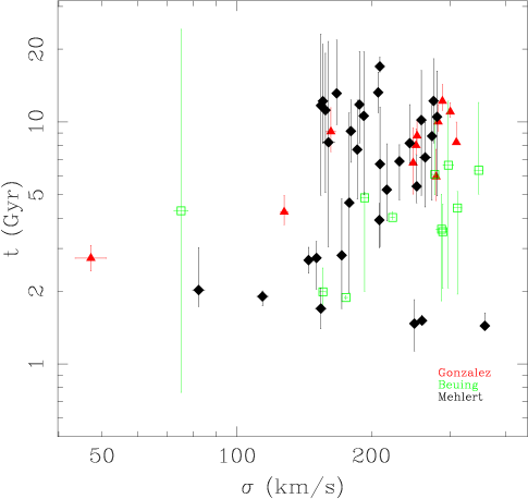
Figure 14: The age–$\sigma$ relation for the high-density sample of Thomas et al. (2005). Diamonds are Coma Cluster ETGs from Mehlert et al. (2003), based on the sample of Mehlert et al. (2000), open squares are cluster ETGs from Beuing et al. (2002), and triangles are cluster galaxies from González (1993, mostly Virgo cluster galaxies).

We now ask why Thomas et al. (2005) find an apparently significant slope in the age–$\sigma$ relation for ETGs in high-density regions while we do not find one for ETGs in the Coma Cluster. We note that their high-density ETG sample contains Coma Cluster ETGs from Mehlert et al. (2003, a compilation of aperture-corrected data from ), Virgo and Pegasus Cluster ETGs from González (1993), and a collection of mostly compact group galaxies from Beuing et al. (2002). We show the age–$\sigma$ data from Thomas et al. (2005) in Figure 14. If we consider only the Coma Cluster galaxies in their sample – the ETG sample of Mehlert et al. (2000) – we do not find an age–$\sigma$ relation. As Thomas et al. (2005) did not publish error bars or confidence levels on their age–$\sigma$ relation, it is difficult to infer the robustness of their result. We therefore cannot say with confidence whether our conclusion truly disagrees with their findings, but we suggest that the Mehlert et al. (2000) data do not by themselves support downsizing in the Coma Cluster.

5.3.3 Why do we disagree with the Coma Cluster RSGs of Nelan et al. (2005)?

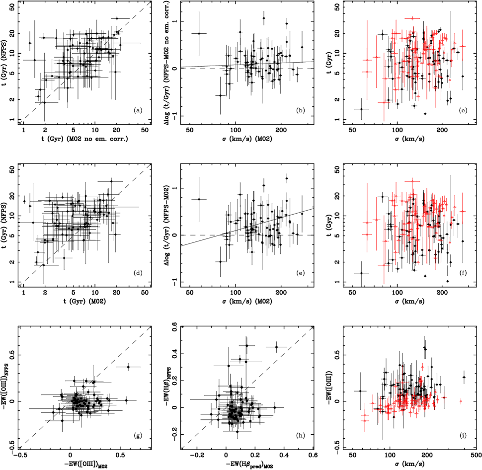
Figure 15: A comparison of ages and emission-line strengths of the Moore et al. (2002) ETG and Nelan et al. (2005) RSG samples for galaxies in common. Panels (a)–(f): A comparison of galaxy ages in the samples. In these panels, the strong outlier GMP 2921 (=NGC 4889) has been removed: its age inferred from the Nelan et al. (2005) data is nearly ten times higher than that inferred from the Moore et al. (2002) sample, with very small formal errors in each sample. The dashed lines represent equality in the ages. The solid lines in panels (b) and (e) are fits to the age differences as a function of $\log\sigma$, accounting for errors along both axes; the slope of the fit in panel (e) is significant, but that in panel (b) is not. In panels (a)–(c) (top row), the $\mathrm{H}\beta$ strengths of the Moore et al. (2002) galaxies have not been corrected for emission, while such a correction has been made in panels (d)–(f) (middle row). Note that the SSP-equivalent ages of the Nelan et al. (2005) sample are on average older than those of the Moore et al. (2002) for galaxies in common, even without the emission-line correction of $\mathrm{H}\beta$. Panels (c) and (f) show the age–$\sigma$ relations for the two samples for galaxies in common to both samples. A comparison of panels (b) and (e) show that neglecting the emission-line correction can impose an age–$\sigma$ relation on the Nelan et al. (2005) RSG sample. Black diamonds: Moore et al. (2002); red triangles: Nelan et al. (2005). Panels (g)–(i): A comparison of emission-line strengths in the samples. (GMP 2921 is included in these panels.) Panels (g) and (h) compare the emission line strengths of the two samples. The predicted $\mathrm{H}\beta$ emission-line strength of the Moore et al. (2002) sample, $-\mathrm{EW(\mathrm{H}\beta)}=-0.6\times\mathrm{EW([O\,\textsc{iii}])}$ (Trager et al., 2000a), is plotted as a function of the measured $\mathrm{H}\beta$ emission-line strength in panel (h). The correlation between the samples is stronger in panel (h) but only marginally significant there (4 per cent probability of being uncorrelated). Panel (i) shows that $\mathrm{EW([O\,\textsc{iii}])}$ is strongly correlated with $\sigma$ in the Nelan et al. (2005) RSG sample, suggesting again that neglecting emission corrections may result in a false detection of an age–$\sigma$ relation.

We next ask why we find a significant age–$\sigma$ relation for the Nelan et al. (2005) Coma Cluster RSG sample but not for the any of the Coma Cluster ETG samples. We compare the large ETG sample of Moore et al. (2002) with the Nelan et al. (2005) sample in Figure 15 for the 71 galaxies in common. In the top and middle rows, we compare the inferred ages of the two samples. In the top row, we compare the ages of the Moore et al. (2002) sample, uncorrected for emission-line fill-in of $\mathrm{H}\beta$, with those of the (uncorrected) Nelan et al. (2005) sample. Apart from a few outliers [and neglecting the strongly deviant galaxy GMP 2921=NGC 4889, which has been removed in panels (a)-(f)], the ages of the two samples are very comparable: the middle panel shows the difference in ages in the samples as a function of velocity dispersion. We do not find a significant slope difference between the samples, merely a small offset, such that the Nelan et al. (2005) ages are $\Delta\log t=0.18\pm 0.13$ dex ($66\pm 31$ per cent) older than the uncorrected Moore et al. (2002) ages. It is important to note that Nelan et al. (2005) rejected galaxies with $\mathrm{EW(\mathrm{H}\beta)}<-0.6$ Å (and $\mathrm{EW([O\,\textsc{iii}])}<-0.8$ Å) from their sample. No galaxy in the Coma Cluster has such strong emission, but certainly small amounts of emission are detected in both the LRIS and Moore et al. (2002) samples. In fact, ten galaxies (out of 97) in the Nelan et al. (2005) data set have detectable emission with $\mathrm{EW(\mathrm{H}\beta)}\leq-0.2$ Å, sufficient to make these galaxies have older SSP-equivalent ages than if their $\mathrm{H}\beta$ strengths had been corrected for this emission. In the middle row of of Figure 15, we compare the ages of the Moore et al. (2002) sample, corrected for emission-line fill-in of $\mathrm{H}\beta$ using the precepts of Trager et al. (2000a, see §2.4), with those of the (uncorrected) Nelan et al. (2005) sample. In panel (e) we find a strong discrepancy in ages which grows stronger with increasing velocity dispersion. As we believe that an emission correction to $\mathrm{H}\beta$ should be applied, we suggest that the age–$\sigma$ relation seen in the Nelan et al. (2005) RSG sample results from their lack of emission-line correction and is not intrinsic to their sample.

Finally, in the bottom row of Figure 15, we compare the emission-line strengths of [Oiii] of the two samples (panel g), the predicted $\mathrm{H}\beta$ emission-line strengths of the Moore et al. (2002) sample with the measured $\mathrm{H}\beta$ emission-line strengths of the Nelan et al. (2005) sample (panel h), and the variation in [Oiii] strength as a function of velocity dispersion (panel i). The [Oiii] strength of the Nelan et al. (2005) sample is correlated with velocity dispersion, reinforcing our suggestion that the age–$\sigma$ relation found in that sample is an artefact of ignoring the (necessary) emission correction. Clearly, larger samples of high-signal-to-noise spectra with careful emission-line correction in the Balmer lines (using, say, the techniques of Sarzi et al., 2006) will be required to resolve this discrepancy completely – but even those techniques are imperfect, as shown by the fact that we detect [Oiii] but not $\mathrm{H}\beta$ emission in our galaxies (which we claim we should have, as it is nearly impossible to have [Oiii] but not $\mathrm{H}\beta$ emission: Yan et al. 2006) using the Sarzi et al. (2006) method (Appendix A.2).

Figure 16: The colour–magnitude relation of Coma Cluster galaxies coded by morphological type. Colours and magnitudes are taken from Beijersbergen (2002) and morphologies from NED. Solid lines are a fit to the colour–magnitude relation; dashed lines are 0.2 magnitudes bluer. Galaxies with types earlier than Sd and Irr galaxies are labelled with their morphological type (I=Irr); Sd and spiral galaxies without specific type are labelled as $\oint$. Galaxies without morphological type in NED are labelled as ”u”. Top panel: E–S0/a galaxies. Middle panel: Sa–Sbc galaxies. Bottom panel: Sc–Irr galaxies and galaxies with unknown morphological types.

Table 9: Deviations from red sequence by morphological type

Morphological type	$\langle\Delta(B-R)\rangle$	$\sigma_{\langle\Delta(B-R)\rangle}$	$N_{\mathrm{gal}}$
cD	$-0.011$	0.024	3
E	0.018	0.007	59
E/S0	0.010	0.014	16
S0	0.006	0.005	146
S0/a	$-0.021$	0.015	27
Sa	$-0.027$	0.014	9
Sab	$-0.160$	0.014	3
Sb–Irr	$-0.029$	0.029	18

Only galaxies with $R<18$ and $\Delta(B-R)>-0.2$ included.

Although we suspect that emission corrections are the primary cause of the discrepancy between the age–$\sigma$ slopes – and thus the detection of downsizing – of all of the Coma Cluster ETG samples and the age–$\sigma$ slope of the Nelan et al. (2005) sample, it is possible that target selection could drive the difference. That is, are the stellar populations of RSGs intrinsically different than those of ETGs? Do colour and morphology drive the presence or lack of an age–$\sigma$ relation? The significant difference between the Nelan et al. (2005) sample and the Jørgensen (1999), Mehlert et al. (2000), Moore et al. (2002), Sánchez-Blázquez et al. (2006b), and LRIS samples is the colour selection of the NFPS galaxies and the morphological selection of all of the other samples. We note that the red sequence contains not only elliptical and S0 galaxies but also disk-dominated early-type spiral galaxies (Fig. 16). We suggest here that a possible solution is that the presence of disc-dominated galaxies in the colour-selected samples could be the cause of the age–$\sigma$ relation found by Nelan et al. (2005, and by extension, ). In Table 9 we examine the deviation from the colour–magnitude relation of Coma Cluster galaxies as a function of morphological type for galaxies that qualify as ‘red-sequence galaxies’ under the criteria of Smith et al. (2004): redder than $-0.2$ magnitudes bluer than the mean colour–magnitude relation in $B-R$. We find that mean deviations from the red sequence become bluer as morphological type becomes later, as might be expected, although the numbers are small. However, Smith et al. (2006) have examined the influence of morphology for a subset of NFPS galaxies by taking only those galaxies with quantitative morphologies and with $B/T>0.5$ (about 35 per cent of the total NFPS sample) and recomputing the $\log\sigma$–parameter relations. They find that a shift of one unit in $B/T$ – i.e., going from pure disc to pure bulge – increases $\log t$ by $0.176\pm 0.026$, which is not enough to erase the age–$\sigma$ relation. Moreover, virtually all of the Nelan et al. (2005) Coma Cluster RSGs are ETGs (only two are typed as Sa in NED). We therefore come to the conclusion that the lack of emission-line corrections to the Balmer lines in the Nelan et al. (2005) sample is likely to be the largest contributor to the difference between that sample and all the others, and that sample selection – RSGs versus ETGs – is unlikely to play a significant rôle in that difference.

To summarise this section, we find no evidence for an age–$\sigma$ or age–mass relation in ETGs in the Coma Cluster. We suggest further that such a relation may not even hold for RSGs in the Coma Cluster, but this requires further high-quality data. We have referred to a significant age–$\sigma$ relation with a positive slope as downsizing of the stellar populations of local ETGs. We do not see significant evidence for such downsizing in Coma Cluster ETGs, and this is not the only environment where this seems to be the case (Kelson et al., 2006). We therefore come to the conclusion that our prediction (i) for the stellar populations of local ETGs in §1 is violated in the Coma Cluster. But we are still left with the question of where the old galaxies are. Have we just missed them, or are they not there, because all early-type galaxies have formed stars recently enough that we see ‘young’ galaxies, as predicted by Kaviraj et al. (2007b)?

5.4 The $Z$-plane and the $\mathrm{[E/Fe]}$-$\sigma$ relation in the Coma Cluster

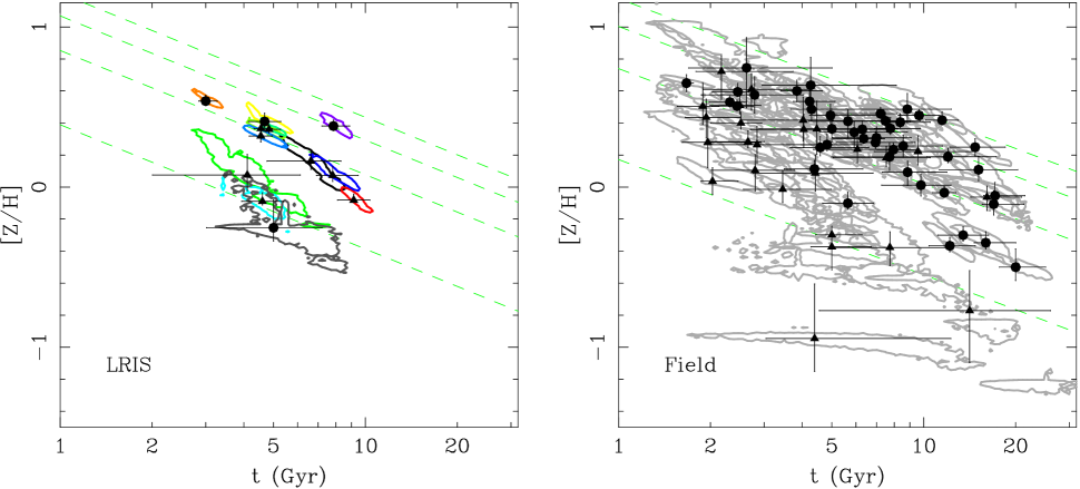
Figure 17: The $Z$-plane for the LRIS Coma Cluster ETG sample (left panel) and our field ETG sample (right panel). Lines of constant $\sigma$, inferred from the $Z$-planes given in Table 7, are shown as dashed lines (bottom to top: 50, 150, 250, 350 $\mathrm{km\,s^{-1}}$).

Finally, we turn to the two relations explored in detail in Paper II: the $Z$-plane and the $\mathrm{[E/Fe]}$–$\sigma$ relation. The $Z$-plane, as discussed above and in Paper II, says that there exists an age–metallicity anti-correlation at each value of $\sigma$, with metallicity increasing with increasing $\sigma$. Note that the $Z$-plane specifically decouples age and $\sigma$, as required from our discussion of the age–$\sigma$ relation above. We plot a nearly face-on projection of the $Z$-plane – the age–metallicity plane – for our LRIS Coma Cluster and field ETG samples in Figure 17. The fact that the $Z$-plane and $\mathrm{[E/Fe]}$–$\sigma$ relation are seen in both field and cluster populations, as found in §4.3.1, suggests that they are a general feature of the stellar populations of ETGs and should therefore be understood in the context of galaxy formation models.

What are the origins of $Z$-plane and $\mathrm{[E/Fe]}$–$\sigma$ relations? We first consider a two-burst model, in which the majority of the mass of ETGs form at high redshift, followed by small bursts of star formation at $z\sim 0.1$–0.3, as discussed above. It is important to recall here that Serra & Trager (2007) have shown that the SSP-equivalent $\mathrm{[Z/H]}$ and $\mathrm{[E/Fe]}$ values are very nearly equivalent to their mass-weighted quantities. This suggests that the $Z$-plane (and $\mathrm{[E/Fe]}$–$\sigma$) relations in the Coma Cluster ETGs were put in place during the initial star formation phases at high redshift and were only mildly perturbed in the secondary star formation events, as long as these secondary events involve only small mass fractions. That is, the secondary bursts must have occurred very recently in order to keep the mass–metallicity and $\mathrm{[E/Fe]}$–$\sigma$ relationships of Coma Cluster ETGs as tight as is found in Figure 10. We discussed the origin of these relations extensively in Paper II. Here we remind the reader that apparently the only available scenarios are (a) early, metal-enriched winds that grow stronger with decreasing ETG velocity dispersion and (b) an IMF slope that becomes flatter with increasing ETG velocity dispersion.

We have shown in §5.2 above that all of the ETGs in the LRIS sample might be assumed to have quenched at $z\approx 0.2$ (although we have ruled this scenario out). Therefore they form a narrow strip in the age–metallicity plane, because they have nearly the same age. Then the question becomes why do they exhibit both a mass–metallicity ($\sigma$–$\mathrm{[Z/H]}$) relation and a $\mathrm{[E/Fe]}$–$\sigma$ relation? In the context of the quenching model, this is because they came from blue, star-forming galaxies that already exhibited these relations (Faber et al., 2007). We therefore speculate that the trends found in Paper II for field ETGs and by Thomas et al. (2005) and Bernardi et al. (2006) for both low- and high-density ETGs – high-$\sigma$ galaxies are older, more metal-rich, and have higher $\mathrm{[E/Fe]}$ – were also exhibited by their blue, star-forming progenitors. We already have evidence of that two of these relations are true for star-forming galaxies: the larger a disc galaxy is, the redder it is (Roberts & Haynes, 1994) – which means the stars formed earlier, as shown by (MacArthur et al., 2004) – and the more metal-rich it is (Tremonti et al., 2004, from SDSS emission-line spectra). We also know that the bulges of large spirals follow the $\mathrm{[E/Fe]}$–$\sigma$ relation (Proctor & Sansom, 2002). Therefore there is already enough evidence to assert that the compositions of ETGs are essentially embedded in their spiral galaxy precursors. If this is the case, that what we are seeing in the LRIS sample is a set of objects of different masses that all got quenched at about the same time. Their chemical compositions follow naturally from their velocity dispersions. In order to fill out the $Z$-plane, then, one needs galaxies that quenched at different times, both earlier and later than our Coma Cluster ETGs – such as the field sample or the sample of Paper II – as seen in Figure 17. This appears to be a more straight-forward explanation of our results than the two-burst model, because the progenitors are clearly identified as blue, star-forming galaxies which we know have the correct scaling relations. Moreover, quenching models of this sort also explain the evolution of the morphology–density relation in clusters (Dressler et al., 1997). But we point out again that massive cluster ETGs are generally old at intermediate redshifts, as discussed above. The quenching model we consider here predicts rather that for the Coma Cluster, most of the ETGs were blue, star-forming galaxies very recently, which we have already rejected in §5.2 above.

We are left in the position of having a reasonable explanation for the origin of the $Z$-plane – that is, that disc galaxies that already possess mass–metallicity and $\mathrm{[E/Fe]}$–$\sigma$ relations are quenched simultaneously – that is ruled out by observations of intermediate-redshift clusters. We have begun to explore whether hierarchical galaxy formation models with detailed chemical evolution can predict these relations (Trager & Somerville, in prep.; Arrigoni et al., in prep.).

6 Summary and conclusions

In §1 we made three predictions for the stellar populations of local ETGs based on observations of RSGs at high redshifts and the results of models of hierarchical galaxy formation:

1. lower-mass ETGs in all environments have younger stellar population ages than high-mass ETGs;

2. ETGs in high-density environments are older than those in low-density environments; and

3. massive ETGs in high-density environments have a small stellar population age spread compared with lower-mass ETGs and those in lower-density environments.

We have tested these predictions using very high signal-to-noise spectra of twelve ETGs spanning a wide range in mass in the Coma Cluster surrounding and including the cD galaxy NGC 4874. Because of the small size of this sample, we have augmented it with larger but less precise samples of ETGs and RSGs in the Coma Cluster.

We find the following results.

1. Coma Cluster ETGs in the LRIS sample are consistent with a uniform SSP-equivalent age of $5.2\pm 0.2$ Gyr (with a possible systematic upper limit of 7.5 Gyr using the Worthey 1994 models), which is identical within the formal errors to the average SSP-equivalent age of a sample of field ETGs drawn from the samples of González (1993), Fisher et al. (1996), and Kuntschner (2000). All Coma Cluster ETG samples are consistent with a single-age population of galaxies, with the exception of the Moore et al. (2002) sample, in which the elliptical and S0 galaxies are each consistent with a single-age population. Differences in calibration onto the Lick/IDS index system and the treatment of possible emission-line corrections of the Balmer lines are primarily responsible for differences in the mean ages between samples. However, the Nelan et al. (2005) RSG sample is inconsistent with a single-age population of galaxies.

2. All Coma Cluster ETG samples are consistent with having no SSP-equivalent age–$\sigma$ or age–mass relation. That is, we see no sign of downsizing in Coma Cluster ETGs. This is not the case in the Nelan et al. (2005) Coma Cluster RSG sample; however, we have shown that this due to neglect of emission-line corrections to the Balmer-line indexes in their sample.

3. The large Coma Cluster ETG sample of Moore et al. (2002) is consistent with the dispersion of SSP-equivalent ages decreasing with increasing velocity dispersion. These age dispersions are typically smaller than those of our field ETG sample at the same velocity dispersion.

4. Field ETGs and all Coma Cluster ETG and RSG samples show both a $Z$-plane and an $\mathrm{[E/Fe]}$–$\sigma$ relation.

Taken together, findings (i)–(iii) mean that predictions (i) and (ii) above does not hold for the stellar populations of Coma Cluster ETGs; only prediction (iii) holds.

We have explored two galaxy formation scenarios to explain these results: (1) one in which old ETGs have recent burst of star formation triggered by an as-yet unidentified process and (2) one in which the on-going star formation in blue galaxies is suddenly shutdown and followed by passive evolution of these galaxies to become the ETGs we see today. We have ruled out the second, ‘rapid quenching’ model on the basis that intermediate-redshift clusters do not have large populations of the massive blue galaxies implied by this model (as previously remarked on by, e.g., Bell et al., 2004b). We therefore consider recent star formation on top of old stellar populations as being the preferred (but not ideal) model. This star formation either happened at $z\sim 0.2$ for most ETGs in the Coma Cluster or the star formation histories of the ETGs were more complex but ‘conspire’ to appear simultaneous using our line-strength dating technique at the present epoch. An open question is, where are the old Coma Cluster ETGs that did not suffer recent star formation? We do find a few galaxies in our sample (GMP 3269 and GMP 3484) whose 68 per cent upper limits on their SSP-equivalent ages approach or exceed 10 Gyr with the W94 models, but the average age at all masses is, again, 5–7 Gyr.

We however must pause and ask whether we have really ruled out downsizing in the Coma Cluster ETG population if all we are detecting is a ‘frosting’ (to use the phrase of Trager et al., 2000b; Gebhardt et al., 2003) of a few percent by mass of young stars on top of a massive population that formed at high redshift. Taking our very simple two-burst models – a young population on top of a 12-Gyr-old population – at face value, we could say yes, that most of the stars formed at an early epoch regardless of their mass. This is contrary to our definition of downsizing. However, we could certainly imagine more complicated ‘frosting’ scenarios in which low-mass galaxies formed the bulk of their stars later than high-mass galaxies – at, say, 8 Gyr rather than 12 Gyr – and then all (or at least most) of the galaxies had a later, small star-formation episode. We admit that it is difficult to test these models with the observations we have presented here. However, others – for example Thomas et al. (2005) and Nelan et al. (2005) – have claimed that they observe downsizing of ETGs directly from their present-day line strengths. It is this precise claim of downsizing that we believe we have falsified, at least in the Coma Cluster. Even if these studies did show ‘downsizing’, the ‘frosting’ scenario calls into question whether this is the same ‘downsizing’ that is seen in lookback studies, as it may only involve a small fraction of the mass. We suggest that at present perhaps only lookback studies (like those mentioned in §1) can detect downsizing in the stellar populations of ETGs.

Are stellar population studies of ETGs therefore not useful? We believe that they are, even if they only address a small fraction of the mass of the population. Our results suggest that something interesting has happened in the Coma Cluster ETGs that appears not to be reproduced by current galaxy formation models or expectations from observations of high redshift galaxies. However, galaxy formation models have not (yet) examined the ages of ETGs in the same way as we determine them locally – i.e., they do not attempt to model $t_{\mathrm{SSP}}$. We (Trager & Somerville, in prep.) are modelling line strengths and SSP-equivalent stellar population parameters to see if our predictions above are still valid when considering the observational quantities presented in this paper. By comparing the results of stellar population analysis of real galaxies to the stellar populations of model galaxies, we will be able to test the validity of our galaxy formation models, helping us to understand the formation processes in real ETGs.

The formation processes of ETGs – those in clusters or in the field – are clearly more complicated than simple, rapid quenching of star formation leading to downsizing. Our results show that we can place new constraints on models of these processes. Of course, considering the ETGs in just one local cluster is a necessary but not sufficient step forward in understanding their formation and evolution. Further clusters must be tested with data of the same quality that (or better than) we have presented here.

Appendix A Calibrating onto the Lick/IDS system

A.1 Initial calibration

As described below, the wavelengths of the Lick/IDS system bandpasses are defined relative to a few template stars. Moreover, the Lick/IDS system is defined at a resolution that varies from about 8 Å at 5000 Å to 10–12 Å at the extreme blue (4000 Å) and red (6400 Å) ends of the system (Worthey & Ottaviani, 1997). As a first step, we choose a template star on which to define the wavelength system. The K1 giant HR 6018 is the template for G and K stars and most galaxies on the Lick/IDS system; we observed this star as well (§2.1). Next we determine the intrinsic resolution of the template $\sigma_{int}$, which is done by fitting (using LOSVD) the spectrum of the template to a digital echellogram of Arcturus (Hinkle et al., 2000). The template spectrum is then smoothed to the Lick/IDS resolution using a variable-width Gaussian filter with an intrinsic dispersion of

$$\sigma_{\mathrm{Lick/IDS}}=3492.88-1.30364\,\lambda+0.000128619\,\lambda^{2}\;\ \mathrm{km\,s^{-1}}$$ (5)

(with $\lambda$ in Å), determined from fitting our spectrum of HR 6018 to the Lick/IDS spectrum of this star. This quadratic fit to the resolution data is very nearly that given by Worthey & Ottaviani (1997). The net smoothing kernel has a width $\sigma_{b}=(\sigma_{\mathrm{Lick/IDS}}^{2}-\sigma_{int}^{2})^{1/2}$ (cf. Proctor & Sansom, 2002).

We next place the wavelengths of the usable Lick/IDS bandpasses on the smoothed template spectrum. Due to the observational material from which it was defined, the Lick/IDS system is not simple to reproduce (see e.g., Worthey & Ottaviani, 1997; Kuntschner, 2000, just to name a few descriptions of the steps required). One particular issue is the wavelength scale of the Lick/IDS system. As described by Worthey et al. (1994) and Trager et al. (1998), the zero-point and scale of the IDS spectra could change between observing runs and even between consecutive exposures as the local magnetic field changed and altered the channel the incoming electrons hit on the IDS detector. Each IDS stellar spectrum was therefore adjusted to have zero redshift and a fixed average wavelength scale, set in AUTOINDEX (Worthey et al., 1994; Trager et al., 1998) by fixing the wavelengths of the strongest two features at (roughly) either end of the spectrum. For cool giants and dwarfs, the (blended head of the) G band and the (blended) Na D doublet were used, defined to have wavelengths of 4306.000 Å and 5894.875 Å respectively; for hot dwarfs, H$\gamma$ was used in the blue; for very cool stars, Ca i was used in the blue.

However, small-scale fluctuations in the wavelength scale still persisted. To overcome this difficulty, AUTOINDEX implemented an index centring scheme that used a high-quality template star to place the bandpasses on each index (Worthey et al., 1994; Trager et al., 1998). There were three templates: HR 6018 for G-K stars, HR 8430 for mid-F and earlier stars, and HR 6815 for early- to mid-M stars. The bandpasses on each template were carefully placed to best reproduce the ‘eye’ system of Burstein et al. (1984). Therefore, the true wavelength definitions of the Lick/IDS passbands can be traced to the wavelength scales of these three stars. The passband definitions of Worthey et al. (1994) and Trager et al. (1998) were based on a comparison of the bandpasses given by the Lick/IDS template stars to the wavelength scales of modern CCD spectra taken by G. Worthey and J. González (see González, 1993).

In the current study, we use a scheme (SPINDEX2; see below) very similar to AUTOINDEX, in which a template star is defined to have the ‘correct’ passband definitions and then is used to centre the indexes on each spectrum of interest. This was necessary in part because it is difficult to calibrate the wavelength scale of LRIS-R spectra in the blue region that concerns us here. The template star must be ‘on’ the Lick/IDS system in order to calibrate the line strengths of the individual objects onto that system. Fortunately, one of our comparison stars is the Lick/IDS K giant standard HR 6018 (§2.1), also the template for cool stars and almost all galaxies in the Lick/IDS system. Using SPINDEX2, we smoothed our spectrum of HR 6018 to the resolution of the Lick/IDS system, after correcting this spectrum to zero velocity as described above. We then shifted the bandpasses given in the original AUTOINDEX template file for HR 6018 by measuring the velocity shifts of each index in the IDS spectrum of HR 6018 (observation 550010, that used as a template for the Lick/IDS system) with respect to the smoothed LRIS spectrum of HR 6018. The wavelength shifts are generally no more than 1.25 Å and typically $\pm 0.125$ to $\pm 0.375$ Å for most indexes in the observed range of the current data (from $\mathrm{CN}_{1}$ to Fe5406).

A.2 Emission corrections

As discussed in previous works (e.g., González, 1993; Goudfrooij & Emsellem, 1996; Kuntschner, 2000), nebular emission lines due to, e.g., low-luminosity AGN (Ho et al., 1997) are common in ETGs. Emission lines of atomic hydrogen, oxygen, and nitrogen can pollute the absorption-line indexes and distort the age and metallicity estimates. The hydrogen Balmer line indexes (H$\delta_{A,F}$, H$\gamma_{A,F}$, $\mathrm{H}\beta$), Fe5015 (which contains both [O iii]$\lambda 4959$ Å and [O iii]$\lambda 5007$ Å) and $\mathrm{Mg}\,b$ (which contains [N i] in its red sideband, Goudfrooij & Emsellem 1996) are all susceptible to emission-line contamination.

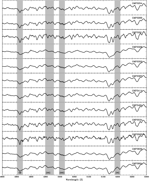
Figure 18: Observed and emission-cleaned spectra of Coma ETGs. Spectra from the 2$\aas@@fstack{\prime\prime}$7 apertures (thick lines) have been fit with Gaussian emission lines and model spectra from Vazdekis (in prep.) and then cleaned of emission (thin lines) using GANDALF (Sarzi et al., 2006). The emission-line index definitions of $\mathrm{H}\beta$, [O iii]$\lambda 4959$ Å, and [O iii]$\lambda 5007$ Å from González (1993) have been over-plotted as grey boxes. A 20 Å-wide ‘index’ around the [N i]$\lambda\lambda 5197.9,5200.4$ Å doublet (Goudfrooij & Emsellem, 1996) has also been over-plotted.

We have used GANDALF (Sarzi et al., 2006) to determine possible emission contamination of our spectra by simultaneously fitting Gaussian emission lines and stellar population model spectral templates (Vazdekis, in prep., based on the spectra of Sánchez-Blázquez et al. 2006a). We accept an emission line to be significantly detected if the ratio of the amplitude of the line to the expected noise $A/N>2$. We find that while nearly of our galaxies (except GMP 3565) have detectable [O iii]$\lambda 5007$ Å emission, we do not detect significant $\mathrm{H}\beta$ emission in any of our galaxies in the 2$\aas@@fstack{\prime\prime}$7 or ‘physical’ $r_{e}/2$ apertures. Nor do we detect any significant [N i]. Because we have not detected $\mathrm{H}\beta$ emission in any galaxy, we have not bothered to correct for emission in the higher-order Balmer lines. We have measured line strengths from the emission-cleaned spectra rather than making the corrections outlined in Trager et al. (2000a) and Kuntschner (2000).

A.3 Measuring line strengths

For each object of interest (star or galaxy), we now measure the line strengths on the (emission-cleaned) spectrum. The spectrum is first smoothed to the Lick/IDS resolution (Eq. 5). Using the systemic velocity given by LOSVD, the bandpasses are placed on the spectrum. For each index, LOSVD is then used to determine the offset between the object and template spectra in a wavelength region that extends 20 Å from the extremes of the index definition. This places the index bandpasses precisely on the Lick/IDS index definition, as described above (thereby following the AUTOINDEX algorithm: Worthey et al., 1994; Trager et al., 1998). Indexes and index errors are then computed from the object spectrum and its variance spectrum using the formalism described by González (1993), namely that an index measured in Å is computed as

$$\mathrm{EW}=\int_{\lambda_{c_{1}}}^{\lambda_{c_{2}}}\!\left(1-\frac{S(\lambda)}{C(\lambda)}\right)\;d\lambda$$ (6)

and an index measured in magnitudes is computed as

$$\mathrm{Mag}=-2.5\log\left[{\left(\frac{1}{\lambda_{c_{1}}-\lambda_{c_{2}}}\right)\int_{\lambda_{c_{1}}}^{\lambda_{c_{2}}}\!\frac{S(\lambda)}{C(\lambda)}\;d\lambda}\right].$$ (7)

Here $\lambda_{c_{1}}$ and $\lambda_{c_{2}}$ are the wavelength limits of the central bandpass, $S(\lambda)$ is the observed flux per unit wavelength in the object spectrum, and $C(\lambda)$ is the linearly-interpolated pseudo-continuum:

$$C(\lambda) = S_{b}\frac{\lambda_{r}-\lambda}{\lambda_{r}-\lambda_{b}}+S_{r}\frac{\lambda-\lambda_{b}}{\lambda_{r}-\lambda_{b}},\ \mathrm{where}$$ (8)

$$S_{b} = \frac{\int_{\lambda_{b_{1}}}^{\lambda_{b_{2}}}S(\lambda)d\lambda}{\lambda_{b_{2}}-\lambda_{b_{1}}}\ \mathrm{and}$$ (9)

$$S_{r} = \frac{\int_{\lambda_{r_{1}}}^{\lambda_{r_{2}}}S(\lambda)d\lambda}{\lambda_{r_{2}}-\lambda_{r_{1}}},$$ (10)

with $\lambda_{b}=(\lambda_{b_{1}}+\lambda_{b_{2}})/2$ and $\lambda_{r}=(\lambda_{r_{1}}+\lambda_{r_{2}})/2$. Errors are then computed using the variance spectrum $V(\lambda)$:

$$\sigma(\mathrm{EW}) = \frac{S_{c}}{C_{c}}\left[\frac{V_{c}}{S_{c}^{2}}+\frac{V_{b}}{C_{c}^{2}}\left(\frac{\lambda_{r}-\lambda_{c}}{\lambda_{r}-\lambda_{b}}\right)^{2}+\frac{V_{r}}{C_{c}^{2}}\left(\frac{\lambda_{c}-\lambda_{b}}{\lambda_{r}-\lambda_{b}}\right)^{2}\right]^{1/2}$$ (11)

$$\sigma(\mathrm{Mag}) = \frac{2.5\times 10^{0.4\mathrm{Mag}}}{\ln(10)(\lambda_{c_{1}}-\lambda_{c_{2}})}\sigma(\mathrm{EW}),$$ (12)

where $\lambda_{c}=(\lambda_{c_{1}}+\lambda_{c_{2}})/2$, $C_{c}=C(\lambda_{c})$, $S_{c}=\int_{\lambda_{c_{1}}}^{\lambda_{c_{2}}}\!S(\lambda)d\lambda$, and

$$V_{c} = S_{c}^{2}/\int_{\lambda_{c_{1}}}^{\lambda_{c_{2}}}\!\frac{S^{2}(\lambda)}{V(\lambda)},$$ (13)

$$V_{b} = S_{b}^{2}/\int_{\lambda_{b_{1}}}^{\lambda_{b_{2}}}\!\frac{S^{2}(\lambda)}{V(\lambda)},$$ (14)

$$V_{r} = S_{r}^{2}/\int_{\lambda_{r_{1}}}^{\lambda_{r_{2}}}\!\frac{S^{2}(\lambda)}{V(\lambda)}$$ (15)

(cf. the discussion in Cardiel et al., 1998). The implementation of this algorithm in Python is called SPINDEX2; when coupled with LOSVD to measure systemic velocities and velocity dispersions (§2.2.1), the program is called SPINDLOSVD.

A.3.1 Reliability of estimated errors

Table 10: Error ratios from 2$\aas@@fstack{\prime\prime}$7-synthesised aperture line strengths

Index	$\langle\sigma_{c}/\sigma_{s}\rangle$	std. dev.
$\mathrm{CN}_{1}$	1.13	0.68
$\mathrm{CN}_{2}$	1.11	0.82
Ca4227	2.21	1.27
G4300	1.52	0.78
Fe4383	1.27	0.87
Ca4455	1.77	1.09
Fe4531	1.54	0.66
$\mathrm{C}_{2}4668$	1.05	0.70
$\mathrm{H}\beta$	1.24	0.74
Fe5015	0.78	0.47
$\mathrm{Mg}_{1}$	0.93	0.60
$\mathrm{Mg}_{2}$	0.67	0.56
$\mathrm{Mg}\,b$	1.08	0.57
Fe5270	1.55	0.93
Fe5335	1.60	0.97
$\langle\mathrm{Fe}\rangle$	1.12	0.95
$\mathrm{H}\delta_{A}$	1.27	0.79
$\mathrm{H}\gamma_{A}$	1.50	0.81
$\mathrm{H}\delta_{F}$	1.40	0.40
$\mathrm{H}\gamma_{F}$	1.64	1.17
$\mathrm{H}\beta_{G}$	1.25	1.07

Col. 1: Index name. Col. 2: Median error ratio, in the sense error inferred from combined spectra divided by standard deviation of index strengths derived from individual exposures. Col. 3: Standard deviation of error ratio.

To check the accuracy of the errors measured from the variance spectra of the averaged spectra as given by Equations 11 and 12 above, line strengths were measured from one-dimensional spectra extracted from each individual exposure. The standard deviation of each index was then determined. Table 10 gives (1) the median and standard deviations of the ratios of the errors in each index computed from the combined spectra and (2) the standard deviations of the index strengths computed from the individual exposures. None of the differences is significant, although some of the means differ from one (e.g., Ca4227 and $\mathrm{Mg}_{2}$). Much of this scatter likely arises from interpolation errors when extracting the one-dimensional spectra from the individual exposures, a problem greatly ameliorated when three images are combined during the extraction. We therefore believe that the error estimates for the LRIS absorption-line strengths are likely to be reliable.

A.4 Calibration onto the stellar Lick/IDS system: offsets and velocity-dispersion corrections

Table 11: Corrections required to bring LRIS stellar indexes onto Lick/IDS system

Index	$\langle\mathrm{(IDS-LRIS)}\rangle^{\mathrm{a}}$	RMS
$\mathrm{CN}_{1}$	$0.0034\pm 0.0008$	$0.0118$
$\mathrm{CN}_{2}$	$0.0063\pm 0.0005$	$0.0064$
Ca4227	$0.034\phantom{0}\pm 0.004\phantom{0}$	$0.057$
G4300	$-0.236\phantom{0}\pm 0.006\phantom{0}$	$0.084$
Fe4383	$-0.033\phantom{0}\pm 0.006\phantom{0}$	$0.094$
Ca4455	$-0.077\phantom{0}\pm 0.004\phantom{0}$	$0.058$
Fe4531	$-0.062\phantom{0}\pm 0.006\phantom{0}$	$0.085$
$\mathrm{C}_{2}4668$	$-0.325\phantom{0}\pm 0.012\phantom{0}$	$0.177$
$\mathrm{H}\beta$	$0.043\phantom{0}\pm 0.004\phantom{0}$	$0.056$
Fe5015	$0.059\phantom{0}\pm 0.010\phantom{0}$	$0.150$
$\mathrm{Mg}_{1}$	$0.0139\pm 0.0005$	$0.0082$
$\mathrm{Mg}_{2}$	$0.0185\pm 0.0004$	$0.0067$
$\mathrm{Mg}\,b$	$0.018\phantom{0}\pm 0.009\phantom{0}$	$0.139$
Fe5270	$0.031\phantom{0}\pm 0.006\phantom{0}$	$0.090$
Fe5335	$0.176\phantom{0}\pm 0.006\phantom{0}$	$0.091$
Fe5406	$0.094\phantom{0}\pm 0.003\phantom{0}$	$0.050$
$\mathrm{H}\delta_{A}$	$-0.143\phantom{0}\pm 0.006\phantom{0}$	$0.083$
$\mathrm{H}\gamma_{A}$	$0.612\phantom{0}\pm 0.015\phantom{0}$	$0.219$
$\mathrm{H}\delta_{F}$	$0.123\phantom{0}\pm 0.004\phantom{0}$	$0.057$
$\mathrm{H}\gamma_{F}$	$0.174\phantom{0}\pm 0.006\phantom{0}$	$0.085$

^aWeighted mean

Because the flux calibration of the present spectra differs from that of the Lick/IDS spectra (which were not fluxed but divided by a quartz lamp; Worthey et al., 1994), small offsets may required to finally bring absorption-line strengths of objects taken with LRIS onto the Lick/IDS system. These offsets are determined by comparing line strengths of the LRIS stars measured with SPINDEX2 to the published values for those stars, as shown in Figure 19. The weighted mean offsets and root-mean-square deviations are given in Table 11. As seen by other authors (e.g., González, 1993; Kuntschner, 2000), most indexes have negligible offsets within the typical errors of the Lick/IDS system. The exceptions are $\mathrm{Mg}_{1}$ and $\mathrm{Mg}_{2}$, for which the Lick/IDS zero-point was set by the quartz lamp used to ‘flux’ the spectra, and $\mathrm{H}\gamma_{A}$, for unknown reasons, although the inferred offset is consistent with that found by both Worthey & Ottaviani (1997) and Kuntschner (2000). Fe5015 has a large scatter for unknown reasons, but it is well within the typical Lick/IDS error. Note that $\mathrm{Mg}_{1}$ and $\mathrm{Mg}_{2}$ may be better fit by a linear relation than a simple offset.

Figure 19: Calibration onto the Lick/IDS system. Line strengths of Lick/IDS stars taken with LRIS were measured with SPINDEX2 (after smoothing to the Lick/IDS resolution, Worthey & Ottaviani 1997) and compared with the published Lick/IDS line strengths (Worthey et al., 1994; Worthey & Ottaviani, 1997). Vertical error bars include uncertainties in the Lick/IDS standard star system (Worthey et al., 1994), scaled using the ‘goodness’ signal-to-noise parameter (Trager et al., 1998) and the number of observations of each star. Offsets from the Lick/IDS system are seen to be small for most indexes, except for the well known offset of $\mathrm{Mg}_{2}$ due to the spectral shape of the quartz lamp used to ‘flux’ the IDS spectra (González, 1993). Dotted and dashed lines indicate the weighted mean offsets and RMS deviations (Table 11); solid lines are lines of equality. Note that some offsets might be better modelled as linear functions of line strength (e.g., $\mathrm{Mg}_{1}$ and $\mathrm{Mg}_{2}$).

Before these offsets are applied to the line strengths of a galaxy, we must first correct them for its velocity dispersion. This is done for the original 21 Lick/IDS line strengths (Worthey et al., 1994) using the multiplicative corrections given by Trager et al. (1998). For the four higher-order Balmer line indexes defined by Worthey & Ottaviani (1997), we use the multiplicative corrections given by Lee & Worthey (2005). For $\mathrm{H}\beta_{G}$ (Jørgensen, 1999), the $\mathrm{H}\beta$ correction given by Trager et al. (1998) was used. As a check on our method, we have compared our velocity-dispersion-corrected indexes (before Lick/IDS system correction) to indexes corrected using the formalism of Kelson et al. (2006), based on broadening templates but not the program spectra, and have found offset and slope differences from our method of less than $1\sigma$ for all indexes except Ca4227, Fe4531, and $\mathrm{H}\delta_{F}$ (offset) and $\mathrm{Mg}\,b$ (offset and slope), where the deviation in the latter index is small ($-0.13$ Å) and only in the strongest (highest-$\mathrm{Mg}\,b$, highest-$\sigma$) objects. Due to the small-to-negligible differences, and more importantly, to be consistent with previous studies, we use the Trager et al. (1998) corrections but note that Kelson et al.’s comments on the suitability of additive rather than multiplicative velocity-dispersion corrections should taken into consideration.

Appendix B Comparison of LRIS data with literature data sources

We now compare our systemic velocities (redshifts), velocity dispersions, and line strengths with those found in the literature. In order to determine the differences most accurately, the LRIS indexes were measured on spectra with apertures matched as closely as possible to the literature data (Sec. 2.1.1). For the study of Mehlert et al. (2003), however, the published $r_{e}/10$ apertures were much too small for nearly all of the galaxies observed in the present sample, so the gradient measures of Mehlert et al. (2000) were used to compute index strengths in 2$\aas@@fstack{\prime\prime}$7-diameter equivalent circular apertures; Fe5270 and Fe5335 indexes and gradients were kindly provided by Dr. D. Mehlert. We also note that the line strengths of Terlevich et al. (1999) are not truly calibrated onto the Lick/IDS system, but rather used the Kuntschner (2000) offsets as a rough correction. This is particularly problematic for the $\mathrm{H}\delta_{A}$ index, as the Kuntschner (2000) study did not include the bluest indexes. Finally, we used the 2$\aas@@fstack{\prime\prime}$7 velocity dispersion measurements to compare with the results of Matković & Guzmán (2005), as velocity dispersion gradients in these galaxies are likely to be nearly flat (cf. Jorgensen et al., 1996).

Table 12: Comparison with other absorption-line strength studies of the Coma Cluster, in the sense Literature$-$LRIS

Quantity	Source	N	Offset	RMS	$\chi^{2}$
$cz_{hel}$	H01	3	$133.32\pm 3.44$	5.95	171.20
$cz_{hel}$	M02	8	$97.51\pm 1.51$	4.28	70.65
$cz_{hel}$	NFPS	7	$123.65\pm 0.78$	2.07	557.06
$cz_{hel}$	ALL	18	$120.00\pm 0.42$	1.78	276.57
$\log\sigma$	D84	4	$-0.022\pm 0.010$	0.020	0.803
$\log\sigma$	G92	1	$0.025\pm\phantom{0.000}$
$\log\sigma$	H01	3	$-0.021\pm 0.006$	0.010	1.847
$\log\sigma$	J99	8	$-0.004\pm 0.003$	0.009	1.220
$\log\sigma$	K01	2	$-0.001\pm\phantom{0.000}$
$\log\sigma$	MG05	6	$-0.014\pm 0.003$	0.007	2.651
$\log\sigma$	M00	3	$0.019\pm 0.009$	0.015	1.594
$\log\sigma$	M02	8	$-0.010\pm 0.001$	0.004	11.490
$\log\sigma$	NFPS	7	$-0.009\pm 0.002$	0.005	4.338
$\log\sigma$	SB06	5	$0.033\pm 0.003$	0.006	10.820
$\log\sigma$	ALL	47	$-0.004\pm 0.000$	0.002	4.743
$\mathrm{CN}_{1}$	NFPS	7	$-0.011\pm 0.002$	0.006	1.986
$\mathrm{CN}_{1}$	P01	5	$-0.040\pm 0.003$	0.006	22.562
$\mathrm{CN}_{1}$	IDS	2	$0.010\pm\phantom{0.000}$
$\mathrm{CN}_{1}$	ALL	14	$-0.024\pm 0.001$	0.004	9.076
$\mathrm{CN}_{2}$	NFPS	7	$-0.020\pm 0.003$	0.008	2.079
$\mathrm{CN}_{2}$	P01	5	$-0.026\pm 0.003$	0.007	10.909
$\mathrm{CN}_{2}$	SB06	5	$-0.008\pm 0.004$	0.009	1.236
$\mathrm{CN}_{2}$	IDS	2	$0.012\pm\phantom{0.000}$
$\mathrm{CN}_{2}$	ALL	19	$-0.018\pm 0.001$	0.004	3.990
Ca4227	NFPS	7	$0.189\pm 0.027$	0.071	1.346
Ca4227	P01	5	$-0.322\pm 0.043$	0.097	2.947
Ca4227	SB06	5	$-0.179\pm 0.023$	0.052	2.527
Ca4227	IDS	2	$-0.249\pm\phantom{0.000}$
Ca4227	ALL	19	$-0.095\pm 0.009$	0.038	1.970
G4300	NFPS	7	$0.067\pm 0.040$	0.107	0.349
G4300	P01	5	$0.108\pm 0.088$	0.198	4.334
G4300	SB06	5	$0.030\pm 0.042$	0.095	1.447
G4300	IDS	2	$0.505\pm\phantom{0.000}$
G4300	ALL	19	$0.057\pm 0.015$	0.065	1.851
Fe4383	NFPS	7	$-0.469\pm 0.053$	0.140	2.252
Fe4383	P01	5	$0.370\pm 0.108$	0.242	2.694
Fe4383	SB06	5	$0.057\pm 0.057$	0.127	0.774
Fe4383	T99	6	$0.547\pm 0.027$	0.065	13.156
Fe4383	IDS	2	$-0.214\pm\phantom{0.000}$
Fe4383	ALL	25	$0.309\pm 0.010$	0.052	4.491
Ca4455	NFPS	7	$-0.384\pm 0.020$	0.053	8.421
Ca4455	P01	5	$-0.091\pm 0.058$	0.130	4.696
Ca4455	SB06	5	$-0.092\pm 0.032$	0.071	0.731
Ca4455	IDS	2	$-0.257\pm\phantom{0.000}$
Ca4455	ALL	19	$-0.258\pm 0.009$	0.040	4.641
Fe4531	NFPS	7	$-0.275\pm 0.032$	0.084	1.891
Fe4531	P01	5	$-0.423\pm 0.093$	0.207	1.968
Fe4531	SB06	5	$-0.383\pm 0.050$	0.113	2.648
Fe4531	IDS	2	$0.153\pm\phantom{0.000}$
Fe4531	ALL	19	$-0.316\pm 0.015$	0.063	1.959

Table 13: continued

Quantity	Source	N	Offset	RMS	$\chi^{2}$
$\mathrm{C}_{2}4668$	FFI	1	$-0.286\pm\phantom{0.000}$
$\mathrm{C}_{2}4668$	M02	8	$0.012\pm 0.062$	0.175	2.036
$\mathrm{C}_{2}4668$	NFPS	7	$0.079\pm 0.061$	0.162	0.253
$\mathrm{C}_{2}4668$	P01	5	$0.565\pm 0.106$	0.237	12.830
$\mathrm{C}_{2}4668$	SB06	5	$-0.962\pm 0.106$	0.237	4.382
$\mathrm{C}_{2}4668$	T99	6	$-0.277\pm 0.030$	0.074	8.030
$\mathrm{C}_{2}4668$	IDS	2	$-1.053\pm\phantom{0.000}$
$\mathrm{C}_{2}4668$	ALL	34	$-0.198\pm 0.010$	0.058	4.580
$\mathrm{H}\beta$	FFI	1	$-0.104\pm\phantom{0.000}$
$\mathrm{H}\beta$	J99	4	$0.178\pm 0.048$	0.096	1.206
$\mathrm{H}\beta$	K01	2	$0.217\pm\phantom{0.000}$
$\mathrm{H}\beta$	M00	3	$0.434\pm 0.055$	0.095	10.795
$\mathrm{H}\beta$	M02	8	$0.008\pm 0.015$	0.042	6.926
$\mathrm{H}\beta$	NFPS	7	$-0.141\pm 0.015$	0.038	2.804
$\mathrm{H}\beta$	P01	5	$0.026\pm 0.048$	0.107	1.821
$\mathrm{H}\beta$	SB06	5	$-0.042\pm 0.026$	0.058	0.481
$\mathrm{H}\beta$	IDS	2	$0.230\pm\phantom{0.000}$
$\mathrm{H}\beta$	ALL	37	$-0.014\pm 0.004$	0.022	3.537
Fe5015	FFI	1	$-0.582\pm\phantom{0.000}$
Fe5015	M02	8	$-0.565\pm 0.047$	0.133	2.919
Fe5015	NFPS	7	$-0.057\pm 0.043$	0.115	0.802
Fe5015	P01	5	$-0.471\pm 0.105$	0.236	2.015
Fe5015	SB06	5	$-0.499\pm 0.069$	0.153	3.814
Fe5015	IDS	2	$-0.072\pm\phantom{0.000}$
Fe5015	ALL	28	$-0.347\pm 0.013$	0.070	2.181
$\mathrm{Mg}_{1}$	J99	4	$0.006\pm 0.001$	0.002	4.607
$\mathrm{Mg}_{1}$	M02	8	$0.002\pm 0.001$	0.003	0.574
$\mathrm{Mg}_{1}$	NFPS	7	$0.015\pm 0.001$	0.003	5.605
$\mathrm{Mg}_{1}$	P01	5	$-0.000\pm 0.001$	0.002	10.325
$\mathrm{Mg}_{1}$	IDS	2	$0.002\pm\phantom{0.000}$
$\mathrm{Mg}_{1}$	ALL	26	$0.006\pm 0.000$	0.001	4.972
$\mathrm{Mg}_{2}$	D84	4	$0.012\pm 0.002$	0.004	3.719
$\mathrm{Mg}_{2}$	G92	1	$0.003\pm\phantom{0.000}$
$\mathrm{Mg}_{2}$	J99	8	$0.006\pm 0.001$	0.003	2.262
$\mathrm{Mg}_{2}$	K01	2	$-0.005\pm\phantom{0.000}$
$\mathrm{Mg}_{2}$	M02	8	$0.008\pm 0.001$	0.003	3.495
$\mathrm{Mg}_{2}$	NFPS	7	$-0.013\pm 0.001$	0.003	2.605
$\mathrm{Mg}_{2}$	P01	5	$-0.036\pm 0.001$	0.003	36.954
$\mathrm{Mg}_{2}$	IDS	2	$0.007\pm\phantom{0.000}$
$\mathrm{Mg}_{2}$	ALL	37	$-0.004\pm 0.000$	0.001	7.404
$\mathrm{Mg}\,b$	FFI	1	$-0.028\pm\phantom{0.000}$
$\mathrm{Mg}\,b$	J99	4	$0.267\pm 0.050$	0.101	1.773
$\mathrm{Mg}\,b$	K01	2	$-0.247\pm\phantom{0.000}$
$\mathrm{Mg}\,b$	M00	3	$-0.152\pm 0.059$	0.102	3.260
$\mathrm{Mg}\,b$	M02	8	$-0.016\pm 0.015$	0.041	2.834
$\mathrm{Mg}\,b$	NFPS	7	$-0.190\pm 0.016$	0.043	4.636
$\mathrm{Mg}\,b$	P01	5	$-0.259\pm 0.046$	0.103	5.239
$\mathrm{Mg}\,b$	SB06	5	$-0.085\pm 0.052$	0.116	1.620
$\mathrm{Mg}\,b$	IDS	2	$0.367\pm\phantom{0.000}$
$\mathrm{Mg}\,b$	ALL	37	$-0.086\pm 0.004$	0.025	3.036
Fe5270	M00	3	$-0.070\pm 0.063$	0.109	0.164
Fe5270	M02	8	$-0.079\pm 0.016$	0.045	2.010
Fe5270	NFPS	7	$-0.115\pm 0.019$	0.049	1.163
Fe5270	P01	5	$-0.051\pm 0.052$	0.117	1.119
Fe5270	SB06	5	$0.050\pm 0.036$	0.082	0.780
Fe5270	IDS	2	$0.248\pm\phantom{0.000}$
Fe5270	ALL	30	$-0.072\pm 0.005$	0.028	1.295

Table 14: continued

Quantity	Source	N	Offset	RMS	$\chi^{2}$
Fe5335	M00	3	$0.030\pm 0.070$	0.121	1.395
Fe5335	M02	8	$-0.091\pm 0.023$	0.064	1.775
Fe5335	NFPS	7	$-0.210\pm 0.021$	0.054	4.050
Fe5335	P01	5	$-0.381\pm 0.060$	0.135	1.942
Fe5335	SB06	5	$0.135\pm 0.041$	0.092	1.805
Fe5335	IDS	1	$0.264\pm\phantom{0.000}$
Fe5335	ALL	29	$-0.114\pm 0.006$	0.035	2.273
$\langle\mathrm{Fe}\rangle$	J99	4	$0.048\pm 0.046$	0.092	0.542
$\langle\mathrm{Fe}\rangle$	K01	2	$-0.213\pm\phantom{0.000}$
$\langle\mathrm{Fe}\rangle$	M00	3	$-0.019\pm 0.047$	0.081	0.978
$\langle\mathrm{Fe}\rangle$	M02	8	$-0.084\pm 0.014$	0.039	2.793
$\langle\mathrm{Fe}\rangle$	NFPS	7	$-0.160\pm 0.014$	0.037	3.689
$\langle\mathrm{Fe}\rangle$	P01	5	$-0.214\pm 0.040$	0.089	2.014
$\langle\mathrm{Fe}\rangle$	SB06	5	$0.091\pm 0.028$	0.062	2.321
$\langle\mathrm{Fe}\rangle$	IDS	1	$-0.004\pm\phantom{0.000}$
$\langle\mathrm{Fe}\rangle$	ALL	35	$-0.087\pm 0.004$	0.022	2.240
$\mathrm{H}\delta_{A}$	NFPS	7	$0.327\pm 0.075$	0.200	1.183
$\mathrm{H}\delta_{A}$	P01	5	$1.140\pm 0.101$	0.225	15.226
$\mathrm{H}\delta_{A}$	SB06	5	$0.239\pm 0.065$	0.144	4.029
$\mathrm{H}\delta_{A}$	T99	6	$0.204\pm 0.024$	0.058	7.200
$\mathrm{H}\delta_{A}$	IDS	2	$0.266\pm\phantom{0.000}$
$\mathrm{H}\delta_{A}$	ALL	25	$0.263\pm 0.010$	0.051	5.914
$\mathrm{H}\gamma_{A}$	NFPS	7	$-0.478\pm 0.059$	0.156	1.754
$\mathrm{H}\gamma_{A}$	P01	5	$-0.028\pm 0.095$	0.213	9.560
$\mathrm{H}\gamma_{A}$	SB06	5	$-0.367\pm 0.062$	0.138	2.049
$\mathrm{H}\gamma_{A}$	T99	6	$-0.092\pm 0.024$	0.058	2.771
$\mathrm{H}\gamma_{A}$	IDS	2	$-0.706\pm\phantom{0.000}$
$\mathrm{H}\gamma_{A}$	ALL	25	$-0.161\pm 0.010$	0.049	3.559
$\mathrm{H}\delta_{F}$	NFPS	7	$-0.139\pm 0.046$	0.121	0.477
$\mathrm{H}\delta_{F}$	P01	5	$0.097\pm 0.068$	0.151	2.277
$\mathrm{H}\delta_{F}$	SB06	5	$0.117\pm 0.037$	0.082	2.381
$\mathrm{H}\delta_{F}$	IDS	2	$0.346\pm\phantom{0.000}$
$\mathrm{H}\delta_{F}$	ALL	19	$0.045\pm 0.014$	0.061	1.491
$\mathrm{H}\gamma_{F}$	NFPS	7	$-0.308\pm 0.026$	0.070	3.158
$\mathrm{H}\gamma_{F}$	P01	5	$0.218\pm 0.059$	0.131	4.310
$\mathrm{H}\gamma_{F}$	SB06	5	$-0.040\pm 0.036$	0.081	0.706
$\mathrm{H}\gamma_{F}$	IDS	2	$-0.498\pm\phantom{0.000}$
$\mathrm{H}\gamma_{F}$	ALL	19	$-0.139\pm 0.011$	0.049	2.559
$\mathrm{H}\beta_{G}$	J99	6	$0.144\pm 0.024$	0.059	1.912
$\mathrm{H}\beta_{G}$	M02	8	$-0.046\pm 0.011$	0.032	5.253
$\mathrm{H}\beta_{G}$	ALL	14	$-0.002\pm 0.007$	0.028	3.821

Col. 1: Quantity of interest. Col. 2: Source of literature data. These abbreviations are shown in Table 3, except ALL is the combination of all studies with data for that quantity. Col. 3: Number of galaxies in common. Col. 4: Weighted mean difference and (random) error of mean, in sense other$-$LRIS. Col. 5: Root-mean-square of difference. Col. 6: $\chi^{2}$ of differences.

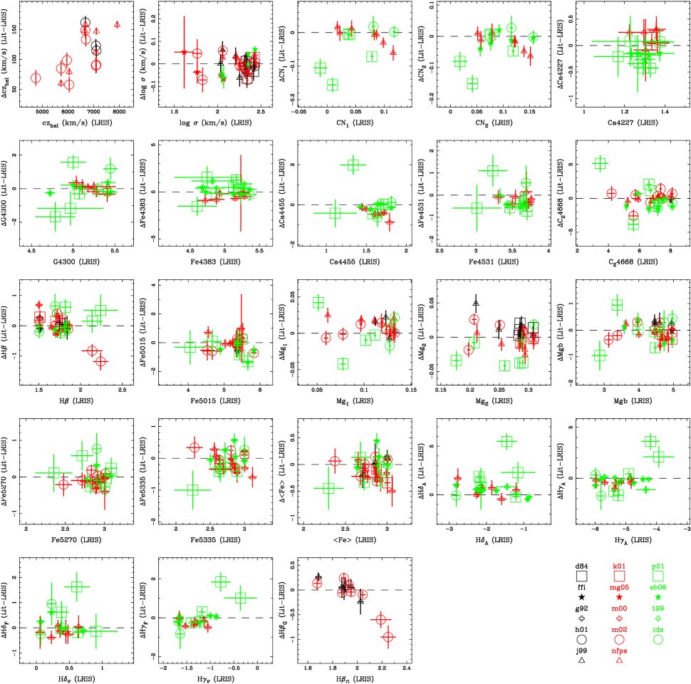
Figure 20: Comparison with literature values. Differences are defined as literature$-$LRIS. Key in lower-right; abbreviations are shown in Table 3.

Figure 20 shows the differences in the sense literature$-$LRIS as a function of LRIS index strength for all of the indexes measured on the LRIS spectra as well as heliocentric velocity $cz_{hel}$ and the logarithm of the velocity dispersion $\log\sigma$. Table 12 gives the mean offsets and the errors in the means ($\sigma_{M}$), in both cases weighted by the errors of the differences (the quadratic sum of the LRIS and literature index errors); the root-mean-squared (RMS) deviation; and the $\chi^{2}$ of the sample difference, computed as

$$\chi^{2}=\frac{1}{N}\sum_{i=1}^{N}\frac{d_{i}^{2}}{\sigma_{i}^{2}}$$ (16)

where $d_{i}$ is the difference of index strengths of galaxy $i$ between a given literature study and LRIS, and $\sigma_{i}$ is the error of the difference. Note that $N<12$ in all cases, as no single literature study contains all of the galaxies in the LRIS sample. The ‘ALL’ entries are error-weighted mean differences for all differences – i.e., the average difference of all literature index values with respect to the LRIS index values.

As we claim that we are precisely on the Lick/IDS system, we can view Table 12 and Figure 20 as guides to the success of the authors of each study in achieving the same calibration. In general, we find that Terlevich et al. (1999) and Poggianti et al. (2001) are not well-calibrated onto the Lick/IDS system, while Moore et al. (2002) and Sánchez-Blázquez et al. (2006b) do a much better job, with some exceptions discussed below. We make no attempt to adjust other studies to our calibration. We note here that our $\mathrm{H}\beta$ strengths are in line with most other studies, excluding the Mehlert et al. (2000) sample, which are clearly much too strong (see below).

Table 15: $\mathrm{H}\beta$ absorption-line strengths of GMP 3329 (NGC 4874) from all sources

Source	$\mathrm{H}\beta$ (Lit)	$\mathrm{H}\beta$ (LRIS)
FFI	$1.410\pm 0.130$	$1.514\pm 0.037$
IDS	$1.307\pm 0.196$	$1.503\pm 0.040$
J99	$1.780\pm 0.120$	$1.512\pm 0.036$
K01	$1.800\pm 0.210$	$1.513\pm 0.033$
M00	$2.140\pm 0.123$	$1.503\pm 0.040$
M02	$1.674\pm 0.132$	$1.503\pm 0.040$
NFPS	$1.519\pm 0.151$	$1.578\pm 0.035$
SB06	$1.496\pm 0.100$	$1.503\pm 0.040$

Col. 1: Source of literature data, as in Table 12. Col. 2: $\mathrm{H}\beta$ strength of GMP 3329 from literature. Col. 3: $\mathrm{H}\beta$ strength of GMP 3329 from LRIS spectra, through the equivalent aperture as described in text.

We are given further confidence in our calibration by examining the literature values of the $\mathrm{H}\beta$ index strengths of the cD galaxy GMP 3329 (=NGC 4874), shown in Table 15. The error-weighted $\mathrm{H}\beta$ index strength in the literature, excluding the significant outlier from Mehlert et al. (2000), is $1.57\pm 0.05$ Å. This is within $1\sigma$ of our $\mathrm{H}\beta$ index strength for this galaxy, suggesting that (at least for this bright galaxy) we are on the Lick/IDS system as well as is possible. However, the $\mathrm{H}\beta$ strength of GMP 3329 (=NGC 4874) in the Mehlert et al. (2000, 2003) studies appears to be much stronger (by $0.64\pm 0.13$ Å) than the mean of all other literature data, including the LRIS measurement; in fact, the Mehlert et al. (2000, 2003) $\mathrm{H}\beta$ strength of this galaxy is higher by more than $0.3$ Å than Jørgensen (1999) and Kuntschner et al. (2001), the strongest other available measurements. It is likely that the explanation for this excess $\mathrm{H}\beta$ strength is over-subtraction of light of this galaxy due to a slit that was too short (Mehlert, priv. comm.). In other words, the signal taken from the end of the slits used to correct for the sky brightness was contaminated by light from the galaxy itself. Given the large size of this galaxy and its surface brightness profile, it is likely that this subtraction results in a too-strong $\mathrm{H}\beta$ absorption-line strength (see Sec. 2.1.1 for details on how we have dealt with this issue). Finally, we note that the SSP-equivalent age of GMP 3329 inferred from the data of Sánchez-Blázquez et al. (2006b) is $\log t=1.02_{-0.14}^{+0.20}$, higher than the age inferred from the LRIS data, $\log t=0.90_{-0.04}^{+0.05}$ (Table 3), even though the $\mathrm{H}\beta$ strengths from the two studies are identical within the errors. This is due to the difference in the measured $\mathrm{Mg}\,b$ strengths: Sánchez-Blázquez et al. (2006b) find $\mathrm{Mg}\,b=4.58\pm 0.26$, while we find $\mathrm{Mg}\,b=4.95\pm 0.04$ (Table 3). We do not know the cause of the difference in this index for this galaxy; all other galaxies in common have very similar $\mathrm{Mg}\,b$ strengths in the two samples, and even in GMP 3329 the strengths of the $\mathrm{H}\beta$, Fe5270, and Fe5335 indexes all match well between the samples.

Detailed examination of Figure 20 shows that the Moore et al. (2002) measurements of GMP 3291 and GMP 3534 are significantly discrepant in $\mathrm{H}\beta$ (and $\mathrm{H}\beta_{G}$). The cause for this discrepancy is not understood, but could be due to slit (in the case of the LRIS spectra) or fibre (in the case of the Moore et al. 2002 spectra) misplacement. Examination of the LRIS slit-alignment images taken immediately before the spectroscopic exposures (Fig. 1) suggests LRIS slit misplacement is unlikely. It is also not due to errors in the velocity dispersion corrections, as both of the galaxies have $\sigma<75\;\mathrm{km\,s^{-1}}$. Given that the $\mathrm{H}\beta$ strengths of both of these galaxies in the Moore et al. (2002) study are extremely low (GMP 3534 has $\mathrm{H}\beta=1.02$ Å in that study, well below the oldest stellar population models; e.g., Fig. 4), it is possible that emission fill-in could be the culprit, but no significant emission is detectable in either galaxy in either study. (Note that a handful of galaxies, typically of low mass, from Moore et al. 2002 have $\mathrm{H}\beta$ strengths that cause them to fall below the oldest stellar population models.) We also note that GMP 3291 is also discrepant with respect to the Poggianti et al. (2001) measurements, but usually in the opposite sense from the comparison with Moore et al. (2002). The LRIS measurements of GMP 3565 are strongly discrepant with respect to the Poggianti et al. (2001) measurements for nearly all indexes. We have confirmed through our slit-alignment images that we have definitely targeted GMP 3565, so LRIS slit misplacement is unlikely to be the culprit for the discrepancies.

Landscape table to go here

Table 3:

Finally, in Table 3 we present absorption-line index strengths and stellar population parameters for all Coma galaxies for six samples: J99, M00, M02, LRIS, NFPS, and SB06 (see Table 3 for definitions). For the M00, SB06, and LRIS samples, we synthesised $2\aas@@fstack{\prime\prime}7$-diameter equivalent circular apertures (§2.1.1); for the other samples, the indexes are taken as published. For simplicity, we present only $\mathrm{H}\beta$, $\mathrm{Mg}\,b$, Fe5270, and Fe5335 index strengths and errors, as these were the indexes used to compute the stellar population parameters. For completeness, we repeat the LRIS indexes, stellar population parameters, and errors here from previous tables. We have not attempted to provide ‘best’ indexes or parameters for galaxies with multiple measurements given the systematic differences between the samples and differences in aperture size (Tables 12 and 3).

References

- Adami et al. (2005a) Adami C., et al., 2005a, A&A, 429, 39
- Adami et al. (2005b) Adami C., Biviano A., Durret F., Mazure A., 2005b, A&A, 443, 17
- Adelman-McCarthy et al. (2007) Adelman-McCarthy J. K., et al., 2007, ApJS, submitted (arXiv:0707.3413)
- Baade & Gaposchkin (1963) Baade W., Gaposchkin C. H. P., 1963, Evolution of Stars and Galaxies. Harvard University Press, Cambridge, MA
- Baldry et al. (2004) Baldry I. K., Glazebrook K., Brinkmann J., Ivezić Ž., Lupton R. H., Nichol R. C., Szalay A. S., 2004, ApJ, 600, 681
- Ball et al. (2006) Ball N. M., Loveday J., Brunner R. J., Baldry I. K., Brinkmann J., 2006, MNRAS, 373, 845
- Beers, Flynn, & Gebhardt (1990) Beers T. C., Flynn K., Gebhardt K., 1990, AJ, 100, 32
- Bell et al. (2004a) Bell E. F., et al., 2004a, ApJ, 600, L11
- Bell et al. (2004b) Bell E. F., et al., 2004b, ApJ, 608, 752
- Beijersbergen et al. (2002) Beijersbergen M., Hoekstra H., van Dokkum P. G., van der Hulst T., 2002, MNRAS, 329, 385
- Bernardi et al. (2006) Bernardi M., Nichol R. C., Sheth R. K., Miller C. J., Brinkmann J., 2006, AJ, 131, 1288
- Bertelli et al. (1994) Bertelli G., Bressan A., Chiosi C., Fagotto F., Nasi E., 1994, A&AS, 106, 275
- Beuing et al. (2002) Beuing J., Bender R., Mendes de Oliveira C., Thomas D., Maraston C., 2002, A&A, 395, 431
- Blanton et al. (2005) Blanton M. R., Eisenstein D., Hogg D. W., Schlegel D. J., Brinkmann J., 2005, ApJ, 629, 143
- Blumenthal et al. (1984) Blumenthal G. R., Faber S. M., Primack J. R., Rees M. J., 1984, Nat, 311, 517
- Brown et al. (2007) Brown M. J. I., Dey A., Jannuzi B. T., Brand K., Benson A. J., Brodwin M., Croton D. J., Eisenhardt P. R., 2007, ApJ, 654, 858
- Bruzual & Charlot (2003) Bruzual G., Charlot S., 2003, MNRAS, 344, 1000
- Bundy et al. (2006) Bundy K., et al., 2006, ApJ, 651, 120
- Burstein et al. (1984) Burstein D., Faber S. M., Gaskell C. M., Krumm N., 1984, ApJ, 287, 586
- Butcher & Oemler (1978) Butcher H., Oemler A., Jr., 1978, ApJ, 219, 18
- Butcher & Oemler (1984) Butcher H., Oemler A., Jr., 1984, ApJ, 285, 426
- Caldwell et al. (2003) Caldwell N., Rose J. A., Concannon K. D., 2003, AJ, 125, 2891
- Cappellari et al. (2006) Cappellari M., et al., 2006, MNRAS, 366, 1126
- Cardiel et al. (1995) Cardiel N., Gorgas J., Aragon-Salamanca A., 1995, MNRAS, 277, 502
- Cardiel et al. (1998) Cardiel N., Gorgas J., Aragon-Salamanca A., 1998, MNRAS, 298, 977
- Cardiel et al. (1998) Cardiel N., Gorgas J., Cenarro J., Gonzalez J. J., 1998, A&AS, 127, 597
- Carlson et al. (1998) Carlson M. N., et al., 1998, AJ, 115, 1778
- Cattaneo et al. (2006) Cattaneo A., Dekel A., Devriendt J., Guiderdoni B., Blaizot J., 2006, MNRAS, 370, 1651
- Cimatti et al. (2006) Cimatti A., Daddi E., Renzini A., 2006, A&A, 453, L29
- Clemens et al. (2006) Clemens M. S., Bressan A., Nikolic B., Alexander P., Annibali F., Rampazzo R., 2006, MNRAS, 370, 702
- Colless et al. (2001) Colless M., et al., 2001, MNRAS, 328, 1039
- Cooper et al. (2006) Cooper M. C., et al., 2006, MNRAS, 370, 198
- Couch & Sharples (1987) Couch W. J., Sharples R. M., 1987, MNRAS, 229, 423
- Cowie et al. (1996) Cowie L. L., Songaila A., Hu E. M., Cohen J. G., 1996, AJ, 112, 839
- Croton et al. (2006) Croton D. J., et al., 2006, MNRAS, 365, 11
- Davis et al. (2003) Davis M., et al., 2003, SPIE, 4834, 161
- De Lucia et al. (2006) De Lucia G., Springel V., White S. D. M., Croton D., Kauffmann G., 2006, MNRAS, 366, 499
- Dressler (1980a) Dressler A., 1980a, ApJ, 236, 351
- Dressler (1980b) Dressler A., 1980b, ApJS, 42, 565
- Dressler (1984) Dressler A., 1984, ApJ, 281, 512
- Dressler et al. (1997) Dressler A., et al., 1997, ApJ, 490, 577
- Drory et al. (2004) Drory N., Bender R., Feulner G., Hopp U., Maraston C., Snigula J., Hill G. J., 2004, ApJ, 608, 742
- Eisenhardt et al. (2007) Eisenhardt P. R., De Propris R., Gonzalez A. H., Stanford S. A., Wang M. C., Dickinson M., 2007, ApJS, 169, 225
- Ellis et al. (1997) Ellis R. S., Smail I., Dressler A., Couch W. J., Oemler A. J., Butcher H., Sharples R. M., 1997, ApJ, 483, 582
- Faber (1973) Faber S. M., 1973, ApJ, 179, 731
- Faber (1977) Faber S. M., 1977, in B. M. Tinsley, R. B. Larson, eds., The Evolution of Galaxies and Stellar Populations. Yale University Observatory, New Haven, p. 157
- Faber et al. (2007) Faber S. M., et al., 2007, ApJ, 665, 265
- Ferreras & Yi (2004) Ferreras I., Yi S. K., 2004, MNRAS, 350, 1322
- Ferreras et al. (2005) Ferreras I., Lisker T., Carollo C. M., Lilly S. J., Mobasher B., 2005, ApJ, 635, 243
- Fisher et al. (1995) Fisher D., Franx M., Illingworth G., 1995, ApJ, 448, 119
- Fisher et al. (1996) Fisher D., Franx M., Illingworth G., 1996, ApJ, 459, 110
- Freedman et al. (2001) Freedman W. L. et al., 2001, ApJ, 553, 47
- Gallazzi et al. (2006) Gallazzi A., Charlot S., Brinchmann J., White S. D. M., 2006, MNRAS, 370, 1106
- Gebhardt et al. (2003) Gebhardt K., et al., 2003, ApJ, 597, 239
- Gerhard et al. (2007) Gerhard O., Arnaboldi M., Freeman K. C., Okamura S., Kashikawa N., Yasuda N., 2007, A&A, 468, 815
- Godwin et al. (1983) Godwin J. G., Metcalfe N., Peach J. V., 1983, MNRAS, 202, 113
- González (1993) González J. J., 1993, PhD Thesis, University of California, Santa Cruz
- Goudfrooij & Emsellem (1996) Goudfrooij P., Emsellem E., 1996, A&A, 306, L45
- Gregg & West (1998) Gregg M. D., West M. J., 1998, Nature, 396, 549
- Guzman et al. (1992) Guzman R., Lucey J. R., Carter D., Terlevich R. J., 1992, MNRAS, 257, 187
- Harker et al. (2006) Harker J. J., Schiavon R. P., Weiner B. J., Faber S. M., 2006, ApJ, 647, L103
- Hinkle et al. (2000) Hinkle K., Wallace L., Valenti J., Harmer D., 2000, Visible and Near Infrared Atlas of the Arcturus Spectrum 3727–9300 Å. Astron. Soc. Pac., San Francisco, CA
- Ho et al. (1997) Ho L. C., Filippenko A. V., Sargent W. L. W., 1997, ApJ, 487, 568
- Holtzman et al. (1992) Holtzman J. A., et al., 1992, AJ, 103, 691
- Hopkins & Beacom (2006) Hopkins A. M., Beacom J. F., 2006, ApJ, 651, 142
- Hudson et al. (2001) Hudson M. J., Lucey J. R., Smith R. J., Schlegel D. J., & Davies R. L., 2001, MNRAS, 327, 265
- Ilbert et al. (2006) Ilbert O., et al., 2006, A&A, 453, 809
- Jørgensen (1999) Jørgensen I., 1999, MNRAS, 306, 607
- Jørgensen & Franx (1994) Jørgensen I. & Franx M., 1994, ApJ, 433, 553
- Jørgensen et al. (1992) Jørgensen I., Franx M., Kjærgaard P., 1992, A&AS, 95, 489
- Jorgensen et al. (1996) Jorgensen I., Franx M., Kjaergaard P., 1996, MNRAS, 280, 167
- Jørgensen et al. (2005) Jørgensen I., Bergmann M., Davies R., Barr J., Takamiya M., Crampton D., 2005, AJ, 129, 1249
- Juneau et al. (2005) Juneau S., et al., 2005, ApJL, 619, L135
- Kaviraj et al. (2006) Kaviraj S., Devriendt J. E. G., Ferreras I., Yi S. K., Silk J., 2006, preprint (astro-ph/0602347)
- Kaviraj et al. (2007a) Kaviraj S., et al., 2007a, ApJS, 173, 619
- Kaviraj et al. (2007b) Kaviraj S., et al., 2007b, MNRAS, in press (arXiv:0709.0806)
- Kelson (2003) Kelson D. D., 2003, PASP, 115, 688
- Kelson (2006) Kelson D. D., 2006, preprint
- Kelson et al. (2000) Kelson D. D., Illingworth G. D., van Dokkum P. G., Franx M., 2000, ApJ, 531, 159
- Kelson et al. (2006) Kelson D. D., Illingworth G. D., Franx M., van Dokkum P. G., 2006, ApJ, 653, 159
- Kennicutt (1998) Kennicutt R. C., Jr., 1998, ARA&A, 36, 189
- Korn et al. (2005) Korn A., Maraston C., Thomas D., 2005, A&A, 438, 685
- Kroupa (2001) Kroupa P., 2001, MNRAS, 322, 231
- Kuntschner (2000) Kuntschner H., 2000, MNRAS, 315, 184
- Kuntschner et al. (2001) Kuntschner H., Lucey J. R., Smith R. J., Hudson M. J., Davies R. L., 2001, MNRAS, 323, 615
- Larson et al. (1980) Larson R. B., Tinsley B. M., Caldwell C. N., 1980, ApJ, 237, 692
- Lauer (1986) Lauer T. R., 1986, ApJ, 311, 34
- Le Fèvre et al. (2005) Le Fèvre O., et al., 2005, A&A, 439, 845
- Lee & Worthey (2005) Lee H.-C., Worthey G. 2005, ApJS, 160, 176
- Łokas & Mamon (2003) Łokas E. L., Mamon G. A., 2003, MNRAS, 343, 401
- MacArthur et al. (2004) MacArthur L. A., Courteau S., Bell E., Holtzman J. A., 2004, ApJS, 152, 175
- Madau et al. (1996) Madau P., Ferguson H. C., Dickinson M. E., Giavalisco M., Steidel C. C., Fruchter A., 1996, MNRAS, 283, 1388
- Maraston & Thomas (2000) Maraston C., Thomas D., 2000, ApJ, 541, 126
- Martin et al. (2005) Martin D. C., et al., 2005, ApJ, 619, L1
- Matković & Guzmán (2005) Matković A., Guzmán R., 2005, MNRAS, 362, 289
- Mehlert et al. (2000) Mehlert D., Saglia R. P., Bender R., Wegner G., 2000, A&AS, 141, 449
- Mehlert et al. (2003) Mehlert D., Thomas D., Saglia R. P., Bender R., Wegner G., 2003, A&A, 407, 423
- Mihos & Hernquist (1994a) Mihos J. C., Hernquist L., 1994a, ApJ, 425, L13
- Mihos & Hernquist (1994b) Mihos J. C., Hernquist L., 1994b, ApJ, 431, L9
- Minkowski (1961) Minkowski R., 1961, AJ, 66, 558
- Mitchell et al. (2005) Mitchell J. L., Keeton C. R., Frieman J. A., Sheth R. K., 2005, ApJ, 622, 81
- Moore (2001) Moore S. A. W., 2001, PhD Thesis, University of Durham
- Moore et al. (2002) Moore S. A. W., Lucey J. R., Kuntschner H., Colless M., 2002, MNRAS, 336, 382
- Nelan et al. (2005) Nelan J. E., Smith R. J., Hudson M. J., Wegner G. A., Lucey J. R., Moore S. A. W., Quinney S. J., Suntzeff N. B., 2005, ApJ, 632, 137
- Noeske et al. (2007) Noeske K. G., et al., 2007, ApJ, 660, L43
- Oke (1990) Oke J. B., 1990, AJ, 99, 1621
- Oke et al. (1995) Oke J. B., et al. 1995, PASP, 107, 375
- Peng et al. (2002) Peng C. Y., Ho L. C., Impey C. D., Rix H., 2002, AJ, 124, 266
- Poggianti et al. (2001) Poggianti B. M. et al., 2001, ApJ, 562, 689
- Press et al. (1992) Press W. H., Teukolsky S. A., Vetterling W. T., Flannery B. P., 1992, Numerical Recipes in C: The art of scientific computing. Cambridge University Press, Cambridge
- Proctor & Sansom (2002) Proctor R. N., Sansom A. E., 2002, MNRAS, 333, 517
- Read & Trentham (2005) Read J. I., Trentham N., 2005, RSPTA, 363, 2693
- Renzini (2006) Renzini A., 2006, ARA&A, 441, 141
- Rix & White (1992) Rix H., White S. D. M., 1992, MNRAS, 254, 389
- Roberts & Haynes (1994) Roberts M. S., Haynes M. P., 1994, ARA&A, 32, 115
- Rood & Baum (1967) Rood H. J., Baum W. A., 1967, AJ, 72, 398
- Rose (1985) Rose J. A., 1985, AJ, 90, 1927
- Rose (1994) Rose J .A., 1994, AJ, 107, 206
- Salasnich et al. (2000) Salasnich B., Girardi L., Weiss A., Chiosi C., 2000, A&A, 361, 1023
- Salpeter (1955) Salpeter E. E., 1955, ApJ, 121, 161