Extracting the spectral function of the cuprates by a full two-dimensional analysis: Angle-resolved photoemission spectra of Bi₂Sr₂CuO₆

Abstract

Recently, angle-resolved photoemission spectroscopy (ARPES) has revealed a dispersion anomaly at high binding energy near 0.3-0.5 eV in various families of the high-temperature superconductors. For further studies of this anomaly we present a new two–dimensional fitting-scheme and apply it to high-statistics ARPES data of the strongly-overdoped Bi₂Sr₂CuO₆ cuprate superconductor. The procedure allows us to extract the self-energy in an extended energy and momentum range. It is found that the spectral function of Bi₂Sr₂CuO₆ can be parameterized using a small set of tight-binding parameters and a weakly-momentum-dependent self-energy up to 0.7 eV in binding energy and over the entire first Brillouin zone. Moreover the analysis gives an estimate of the momentum dependence of the matrix element, a quantity, which is often neglected in ARPES analyses.

I Introduction

Angle-resolved photoemission spectroscopy (ARPES) has been an excellent tool for studying many-body interactions in two-dimensional strongly-correlated systems Group:Review . Recently, ARPES studies revealed a new energy scale in the form of a large dispersion anomaly near 0.3-0.5 eV below $E_{F}$, seen in various families of cuprates, at a wide range of doping and measuring conditions (e.g. photon energy) CCOC:Filip ; HEA:Non ; HEA:Lanzara ; HEA:Donglai ; HEA:Valla ; HEA:Pan ; HEA:Chang . Given its phenomenological behavior, this anomaly could be important to understand the nature of high-temperature superconductivity. However, its origin is still under debate CCOC:Filip ; HEA:Non ; HEA:Lanzara ; HEA:Donglai ; HEA:Valla ; HEA:Pan ; HEA:Chang ; Hubbard:Hanke ; Hubbard:Alexandru ; tJ:Manousakis ; DMFT:Byczuk ; Magnon:Markiewicz ; crossover:Wang ; InplaneOptical:Chubukov .

From earlier study, this energy scale is in the range where the J scale coherent band is split from the t scale incoherent electronic structure structure due to Mott-Hubbard physics Review:Dagotto . Newer data seem to suggest that there is momentum dependence even in the incoherent part of the electronic state at higher energy, even though the uncertainty due to matrix element distortion has been raised ME:Inosov ; ME:Kordyuk . An interesting question would then be whether one can take the data in its face value and make a global analysis in terms of self-energy. This has several advantages. First, it explores a new ARPES methodology to extract and parameterize many body effects in complex materials. Second, it allows one to make a comparison with the information extracted from optical reflectivity measurements InplaneOptical:vanderMarel ; InplaneOptical:Chubukov ; InplaneOptical:Erik ; InplaneOptical:Hwang where one would not expect the same kind of matrix element effects as in ARPES. This would be a good consistency check. Last, it will help us to gain insights of many-body effect and matrix element effect even in the ARPES context. Such an approach is non-trivial to implement due to the difficulties encountered with standard data analysis techniques, which can introduce strong artifacts in the extracted quantities of interest, most notably the self-energy. An improved quantitative analysis of the experimental data would undoubtedly help to advance our understanding.

It is a technical challenge to extract the spectral function, which contains the information of the interactions, from ARPES data. The main problem is the lack of general analytic expressions for individual momentum distribution curves (MDCs) or energy distribution curves (EDCs). Non-Lorentzian MDC peak shapes are common even in simple situations, e.g. in the case of non-linearly dispersing bands. Energy distribution curves are even more delicate to analyze since their precise shape is determined by the energy dependence of the self-energy, i.e. the quantity that should be extracted from the analysis. Further complications arise from the finite instrumental energy and momentum resolution, low-counting statistics, or matrix element effects. All these complications cause discrepancies between the commonly used MDC or EDC analyzes, which become, particularly pronounced at high binding energy HEA:Lanzara ; HEA:Donglai . Different problems arise in the other important regime near the Fermi level where the feature of interest (e.g. the scattering rate near the Fermi level) are comparable in width to the instrumental resolution. In this case, one needs to estimate the combined effect of energy and momentum resolution on a single EDC or MDC, which can only be done approximately or by restricting the self-energy to simple analytic forms RhO4:FelixB ; RuO4:Nik .

In this paper we introduce a new two-dimensional (2D) analysis scheme, which allows us to extract an empirical spectral function of a strongly interacting system over an extended energy range. The method is applied to high-statistics ARPES data from strongly-overdoped Bi₂Sr₂CuO₆ (Bi2201) single crystals. The feature of interest will be the high-energy anomaly around 0.3-0.5 eV. We will not concern ourselves with the low energy anomaly or ”kink” (0.03-0.09eV), which can be highly momentum dependent Bi2212:Tanja . Since the width of the high-energy anomaly is large compared to the experimental resolution, we will neglect the influence of instrumental broadening. Our analysis qualitatively reproduces all the basic features seen in both MDC and EDC analysis and shows that the spectral function of Bi2201 can be empirically parameterized by a simple and compact set of tight-binding parameters fitted to local-density-approximation (LDA) calculations and a weakly momentum-dependent self-energy. Further, this extracted self-energy is in reasonable agreement with the one extracted from optical reflectivity measurement InplaneOptical:Erik . This finding provides a new approach to understanding many-body effects beyond the narrow energy range around the Fermi level which has traditionally been the focus of ARPES studies.

We have selected strongly-overdoped Pb-substituted Bi2201 for this study for several reasons: (a) in the overdoped regime, there is no complication from pseudogap behavior near the antinodal region or from polaronic behavior; hence the 2D analysis can be applied to the whole Brillouin Zone (BZ); (b) bi-layer splitting effects are absent in this single-layer cuprate and superlattice effects are largely suppressed by the Pb content; (c) measurements at low temperature, where thermal broadening is small, are not complicated by the effects of the superconducting gap.

II Experiment

We have measured single crystals of Pb-substituted Bi2201. The overdoped (OD) samples with composition, Pb_0.38Bi_1.74Sr_1.88CuO_6+δ, are non-superconducting ($\rm T_{c}$ $<$ 4 K). ARPES data were collected on a Scienta R4000 electron energy analyzer at the Advanced Light Source (ALS) with photon energies of 42 and 55 eV and a base pressure of $4\times 10^{-11}$ torr. This analyzer has the advantage of a large-angle window which can cover the band dispersion across the entire BZ. Samples were cleaved in situ in the normal state at the measurement temperature of 20K. The energy resolution was set to 13-18 meV. The average momentum resolution at these photon energies was   0.021 Å^-1 (or 0.35^∘). The linear polarization of the light source is fixed to be in-plane along (0,0) to ($\pi$,$\pi$) through out the measurement. Note that the fitted matrix element, which will be shown in the following, should be referred to this particular experimental geometry.

III 2D analysis

Conventionally, ARPES data from cuprates are analyzed by fitting large numbers of one-dimensional intensity profiles at constant energy (MDCs) or constant momentum (EDCs) using simple analytical functions. However, such an analysis of EDCs or MDCs has limitations which will be discussed in more detail in Appendix A (Fig. 5). Attempting to go beyond the conventional EDC or MDC analysis , we use here a full 2D analysis which will be explained in the following. Our starting point is the common expression for the photocurrent within the sudden approximation Group:Review :

$$I({\bf k},\omega)=I_{0}({\bf k},\nu,{\bf A})f(\omega){\mathcal{A}}({\bf k},\omega)$$ (1)

where $I_{0}({\bf k},\nu,{\bf A})$ is proportional to the squared one-electron matrix element and depends on in-plane electron momentum ${\bf k}$, the energy ($\nu$) and polarization (or vector potential, ${\bf A}$) of the incoming photon, $f(\omega)$ is the Fermi function. $\mathcal{A}({\bf k},\omega)$ is the single-particle spectral function that contains all the corrections from the many-body interactions in the form of the self-energy, $\Sigma({\bf k},\omega)$,

$${\mathcal{A}}({\bf k},\omega)=\frac{(-1/\pi)\ \ \textrm{Im}\Sigma({\bf k},\omega)}{[\omega-\epsilon^{0}_{k}-\textrm{Re}\Sigma({\bf k},\omega)]^{2}+[\textrm{Im}\Sigma({\bf k},\omega)]^{2}}$$ (2)

where $\epsilon^{0}_{k}$ is the bare band dispersion. Note that we have neglected the instrumental resolution in Eq. 1.

This form is intrinsically multi-dimensional. Given that ARPES data are collected with most modern spectrometers in parallel as a function of energy and one momentum coordinate, it appears to be an artificial oversimplification to analyze the data by fitting single line profiles. Instead, the analysis presented below is an attempt to fit ARPES data at once in 2D images. This analysis assumes a simple form of the bare band dispersion given by a tight-binding approximation of LDA calculations HEA:Non . For simplicity , we will also assume weak momentum dependence of the self-energy (i.e. over a sufficiently small k space range, $\Sigma({\bf k},\omega)$ $\rightarrow$ $\Sigma(\omega)$) where in the next section, we will show that this is a reasonable assumption. However, our analysis does not assume any particular form of the self-energy and the matrix element. This is achieved by assigning an individual fit parameter for real and imaginary part of the self-energy to every measured energy point and a fit parameter for the matrix element to every momentum point.

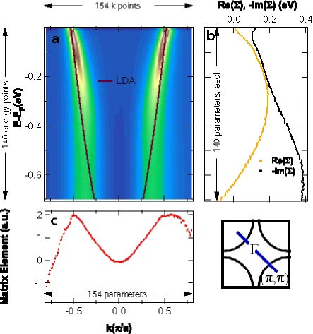
Figure 1: (Color online) a) Image plot of the fitted intensity from the 2D analysis of ARPES data of OD Bi2201 along the nodal direction (0,0) to ($\pi,\pi$) where the solid line shows a bare dispersion derived from LDA. b) The fitting parameters for real and imaginary parts of self-energy. c) The fitting parameters for the matrix element.

This is illustrated in Fig. 1 showing an image plot of the fitted intensity together with the values of the fitting parameters for the self-energy ($\Sigma$) and matrix element ($I_{0}({\bf k},\nu,{\bf A})$). The bare dispersion $\epsilon^{0}_{k}$ derived from LDA is shown as solid line. Starting with an ARPES image of 154 by 140 data points in momentum and energy respectively, the least-square fit of this Fig. 1 includes 154 parameters for each k point for the matrix element, 140 parameters for each energy point of $\textrm{Im}\Sigma$ and $\textrm{Re}\Sigma$, and a few additional parameters for an overall intensity and background, i.e. a total of about 440 parameters. This number seems high, but it is justifiable given that the number of data points is much larger. In the above example, we have $140\times 154$ = 21560 data points corresponding to about 50 points per parameter. Fitting a single MDC with a Lorentzian on a constant background requires more parameters per data-point.

We stress again that this 2D analysis on Bi2201 will focus on the high-energy anomaly whose energy scale of 0.3-0.5eV is larger than the energy resolution. We will not focus on the energy scales below 0.1 eV where it has been shown that the self-energy is strongly momentum dependent Bi2212:Tanja . We also note that Kramers-Kronig consistency of the self-energy is not implemented in the fitting procedure. This will be discussed in more detail in Appendix B.

IV Results

IV.1 Extracting Spectral Function and Self-energy

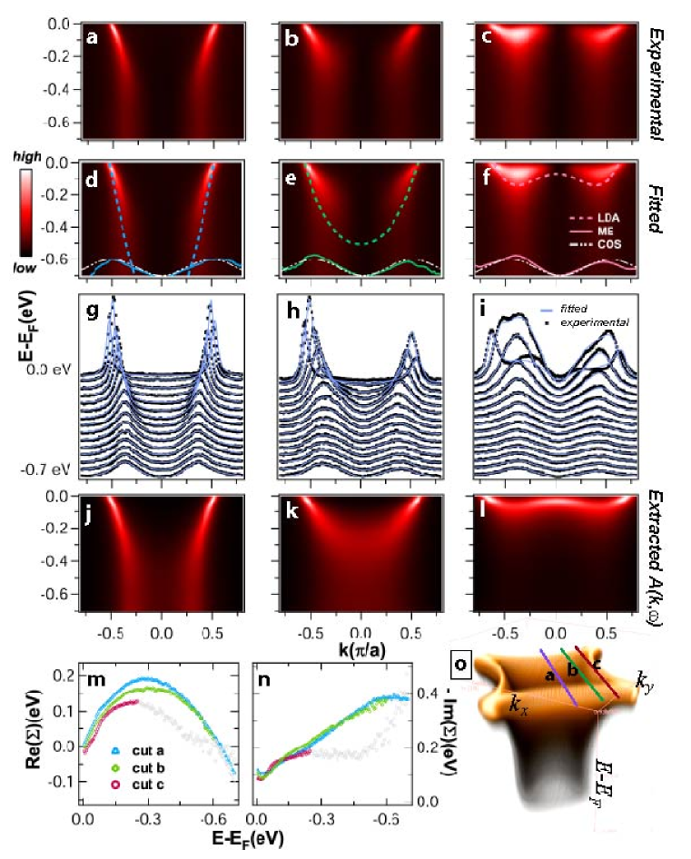
Figure 2: (Color online) On the first row, a)-c) are the experimental ARPES data along momentum direction as indicated by the band shown in bottom right. On the second row, d)-f) are the corresponding image plots of the fitted intensity from the 2D analysis. The thicker color dashed lines are the dispersions generated from the tight-binding parameters from LDA calculation (LDA) given above. The solid color lines are the matrix elements (ME) obtained from the 2D analysis where the smaller white dashed lines are the empirically guessed form of the matrix element in the form of a cosine function (COS). On the third row, g)-i) are the MDCs of raw data (black dots) and corresponding image plot of the fitted intensity (blue line). Taken out the matrix element effect and background, j)-l) are the corresponding extracted spectral function ($\mathcal{A}({\bf k},\omega)$) from the 2D analysis. m) and n) are the extracted real and imaginary parts of the self-energy in Eq. 2 for the cuts a, b and c; the extracted values are plotted in colors up to the energy not far from the bottom of the bare band (up to 0.6 eV for cut b and 0.25 eV for cut c) and in grey at higher energy. o) shows the band structure generated from the tight-binding parameters and the self-energy along the nodal direction.

We now apply the 2D analysis to several k-space cuts as shown in Fig. 2. The ARPES experimental data are shown in the first row (Fig. 2(a)-2(c)), taken with photon energy 42 eV. We deliberately choose the spectra which would be difficult to analyze by MDC or EDC analysis alone because they have regions where EDC (see, cut a) and MDC (see, cut c) peaks are not be well-defined. We then apply the 2D analysis on these data using the following tight binding description of the bare dispersion: $E(k)=-2t[cos(k_{x}a)+cos(k_{y}b)]-4t^{\prime}cos(k_{x}a)cos(k_{y}b)-2t^{\prime\prime}[cos(2k_{x}a)+cos(2k_{y}b)]-E_{F}$ where $t=0.435,t^{\prime}=-0.1,t^{\prime\prime}=0.038,$ and $E_{F}=-0.5231$ eVHEA:Non ; TB:comment . Since the background is small ($\sim$5% of the spectral intensity at $k_{F}$) and flat in this chosen energy range (EDCs are shown in Fig. 1(c) of Ref. HEA:Non ), we use a constant energy-and-momentum-independent background for this particular data.

The corresponding fits are very well in agreement as shown in the second row (Fig. 2(d)-2(f)) while MDCs of the fit and the raw data are shown in the third row (Fig. 2(g)-2(i)). From this 2D analysis, we then extract the spectral function ($\mathcal{A}({\bf k},\omega)$) which is shown in Fig. 2(j)-2(l). These plots of extracted spectral function do not contain the matrix elements anymore but still show the high-energy dispersion anomaly. Further, the optics matrix element effect is different and much weaker and an extracted self-energy of the same Bi2201 sample obtained from optical reflectivity measurement shows a reasonable agreementInplaneOptical:Erik . The above analysis as well as the consistency with optics suggests that there is a real many body anomaly in the energy range. We should note that although we agree that matrix element effects may distort the spectral line shape (e.g. the difference between Fig. 2(a)-2(c) and 2(j)-2(l), respectively), they can hardly explain the high-energy anomaly as put forward by Ref. ME:Inosov . Possibly, the effects observed and discussed there are influenced in a non-negligible way by multi-band effects known in Bi2212 and YBCO.

The self-energies ($\Sigma$) extracted by the 2D analysis in Fig. 2(m) and 2(n) show only weak momentum dependence over the most relevant energy range. Pronounced differences between the three cuts shown in Fig. 2 are only found at energies below the band bottom. However, these parts of the self-energies (see grey symbols in Fig. 2(m) and 2(n)) should not be overestimated as they will not contribute much spectral weight to the spectra. Hence, the ARPES data of this OD Bi2201 system can approximately be parameterized in a simple form using tight-binding parameters and the self-energy along the nodal direction without losing much information of the spectral weight distribution throughout energy and momentum space. Therefore, we can calculated a good approximation of the full 3D intensity distribution from this information as shown in Fig. 2(o).

This is intriguing finding that the information of the ARPES spectra of the OD Bi2201 system throughout the BZ can be much deduced into a very simple and compact set of tight-binding parameters and a weakly-momentum dependent self-energy. Given its simplicity, we believe that this finding will reveal us more of the nature of the interactions in cuprates, especially of the high-energy anomaly CCOC:Filip ; HEA:Non ; HEA:Lanzara ; HEA:Donglai ; HEA:Valla ; InplaneOptical:Chubukov .

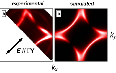
Figure 3: (Color online) a) shows the experimental Fermi surface map of OD Bi2201 where the light polarization, E, is along the nodal direction, $\Gamma\rightarrow Y$. b) shows the Fermi surface map which is constructed from the extracted spectral function and the empirical guessed matrix element.

IV.2 Matrix Element Effect

Although the matrix element effect is known to exist in ARPES measurement ME:Bansil , matrix elements are often neglected in the analysis of ARPES data, whereas they are naturally embedded in the presented 2D analysis. This uniquely allows one to separate the spectral function from matrix element effects as demonstrated in Fig. 2(j)-2(l). The behavior of the matrix elements, as obtained from our analysis is shown in arbitrary units at the bottom of Fig. 2(d)-2(f) by solid colored lines. The line shape of the extracted matrix element are usually smooth in the region of $|k|<k_{F}$ but will get noisy outside the Fermi surface. This can be explained by the following. In the region outside $k_{F}$, there is not much of the spectral weight to be fitted and hence, we emphasize that only in region of $|k|<k_{F}$, the extracting of matrix element should be counted. As shown in Fig. 2(d)-2(f), the extracted matrix elements in the $|k|<k_{F}$ region show similar line shape. Here, we empirically guess the form of the matrix element to be in the form of $\alpha(1-\cos(2\vec{k}\cdot a\hat{s}))/2$ where $\hat{s}$ is the direction of the light propagating vector (perpendicular to the polarization, $\hat{E}$) and $\alpha$ is an arbitrary constant along $\hat{s}$; these empirical forms are shown as the white dash lines on top of the extracted matrix elements.

As a cross test of our analysis, we construct the Fermi surface using the extracted spectral function and the empirical form of the matrix element with $\alpha=1$. In Fig. 3, we compare this constructed Fermi surface of OD Bi2201 (Fig. 3(b)) to the experimental data (Fig. 3(a)). The one-step model calculation by Mans et. al. for Bi2212 system shadow:Mans shows a similar intensity distribution. Although this empirical form of the matrix element may be oversimplified, some of main features (e.g. the suppression of the intensity along $\Gamma\rightarrow Y$) could already be captured by this form.

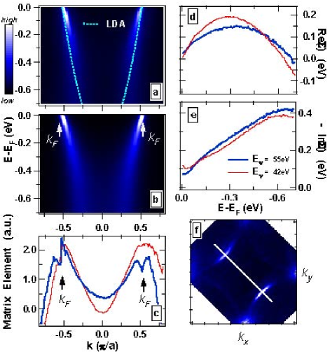
Figure 4: (Color online) Measured at photon energy, $E_{\nu}$ = 55 eV, a) shows the experimental ARPES data along (0,0) to ($\pi,\pi$) direction as indicated in f) where the dash line shows the tight-binding band from LDA calculation used as bare dispersion. b) shows the corresponding extracted spectral function ($A(k,\omega)$) from the 2D analysis. c) show the extracted matrix elements of the data taken at $E_{\nu}$ = 55 eV (solid line) and 42 eV (dash line) where the areas under the graphs between $k<|k_{F}|$ are normalized to be the same. d) and e) are the extracted $\textrm{Re}\Sigma$ and $\textrm{Im}\Sigma$ of the data taken at $E_{\nu}$ = 55 eV (solid line) and 42 eV (dash line). f) shows the Fermi surface map.

IV.3 Comparison of Data Measured at Two Different Photon Energies

To check further on the robustness of the 2D analysis, we perform ARPES measurement with a second photon energy (55 eV) (Fig. 4), taken on a different sample and compare them with the 42 eV data shown in Fig. 2 and 3. A clear difference in intensity modulation of Fermi surface maps with these two photon energies is evident from a comparison of Fig. 3(a) and 4(f). We then apply the 2D analysis on this 55 eV data. As shown in Fig. 4(c), the extracted matrix element of 55 eV data (solid line) looks different in curvature from the 42 eV data as expected from the different appearance of the two Fermi surface maps. And, as shown in Fig. 4(d) and 4(e), the extracted self-energies of 42 eV and 55 eV show the same line shape but have slight differences in energy value, giving the impression of error bar from this 2D analysis. Notice that the comparison of the extracted $\textrm{Im}\Sigma$ gives better agreement than $\textrm{Re}\Sigma$. We believe that one possibility might be due to that $\textrm{Re}\Sigma$ couples directly to the k-dependent bare band dispersion $\epsilon^{0}_{k}$ (see Eq. 2) and hence a slight misalignment of k space from experiment or any $k_{z}$ dependent effects from different photon energies 3D:Takeuchi could cause a larger error bar to the extracted value of $\textrm{Re}\Sigma$.

V CONCLUSION

We presented a 2D analysis method for ARPES data, which allows one to extract self-energies and matrix elements in more general situations and with much higher reliability as compared to standard line-by-line analyses. The method has been applied to high-statistics ARPES data from strongly overdoped Bi2201. It was found that the spectral function at high energies is well approximated over the entire Brillouin zone by a very simple and compact set of tight-binding parameters and a weakly-momentum dependent self-energy. We believe that this method will be useful in the analysis of ARPES data from many systems and may provide us with more information for improving understanding of many-body interactions in cuprates.

Appendix A MDC and EDC analaysis

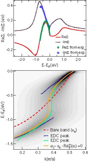
Figure 5: (Color online) a) shows the real (solid line) and imaginary (dash line) parts of self-energy used to construct the spectral image shown in b). In Fig. b), we compare the MDC-peak (fine dash line) and EDC-peak (medium-size dash line) dispersions with the input band dispersion (solid line). We note that $\textrm{Re}\Sigma$ and $\textrm{Im}\Sigma$ shown in a) satisfy the Kramers-Kronig relation where the diamond and circle symbols represent extracted real and imaginary parts of self-energy, respectively from Fig. 2(m) and 2(n) of cut a.

MDC and EDC analysis is the conventional method to analyze each one dimensional (1D) spectrum of ARPES data. For an example, a peak position of an EDC could represent the band dispersion and its peak width could represent the scattering rate. However, a common problem occurring with these analysis is that a good fitting of an experimental data set cannot be done empirically but often needs an additional theoretical modeling. To get a precise fitting of an EDC, or an 1D energy-dependent spectrum at a fixed momentum, one will need to know its self-energy as a function of energy (i.e. the quantity that should be extracted from the analysis). Similarly for an MDC, one will need to know the matrix element as a function of momentum. Therefore, when the matrix element effect is pronounced or the self-energy is strongly energy dependent, fitting an MDC or EDC with a simple function (e.g. Lorenztian) will not give a good agreement. Note that the implementation of Kramers-Kronig transformation on self-energy can help to avoid having assumption on the self-energy form and make it empirical selfenergy:Norman ; selfenergy:Chul . However, such transformation has limitation and requires the spectrum from $-\infty$ to $+\infty$ in energy while clean data in doped cuprates can only be obtained from Fermi level up to around half of band width in binding energy before complications from valance bands come in HEA:Non .

As shown in Fig. 5, to compare the MDC and EDC peak dispersions, we have constructed ARPES data (Fig. 5(b)) from the generated Kramers-Kronig satisfied self-energy in Fig. 5(a) and the same matrix element as used in Fig. 3(b). To generate this self-energy in Fig. 5(a), we start out with our extracted self-energy of the nodal spectrum (cut a) in Fig 2(m) and 2(n) and then we extend it in an arbitrary but Kramers-Kronig consistant way. Given that all information is known, the solution of poles ($\omega-\epsilon_{k}-Re\Sigma(\omega)=0$) can be traced precisely as shown in Fig. 5(b). Although MDC and EDC peak dispersions show agreement for small binding energy less than 0.3 eV, the discrepancy is large at energy above the high-energy anomaly ($>$ 0.3 eV.) In Fig. 5, where the band is very dispersive, EDC analysis fails to track the band since the EDC peak is not well-defined. On the other hand (not shown), when the band is shallow (e.g. Fig. 2(c)), MDC peak dispersion may fail to describe the band dispersion (discussed also in Ref. HEA:Donglai .)

Appendix B Kramers-Kronig relation

From Eq. 2, by causality, the real and imaginary part of self-energy are related by Kramers-Kronig relations. In principle, if the full spectral function ${\mathcal{A}}({\bf k},\omega)$ is known, one could perform an inversion to obtain the full self-energy using the Kramers-Kronig transformation selfenergy:Norman ; selfenergy:Chul . However, such transformation has limitations and requires the spectrum from $-\infty$ to $+\infty$ in energy. Unfortunately, clean ARPES data from doped cuprates can usually be obtained from Fermi level to around half of the band width where complication of valance bands will come in HEA:Non .

Attempting to use the Kramers-Kronig transformation on self-energy of doped-cuprate data is then required to have a cut-off/extension model at energies above the existing data points KK:Kordyuk . However a cut-off/extension model is difficult to be justified and the result can vary substantively, depending on the cut-off/extension model used. For example, with a certain assumption of cut-off/extension model, Ref. ME:Inosov claims that the self-energy extracted by using LDA as a bare band cannot satisfy Kramer-Kronig relation. In contradiction to the claim, here, by extending the self-energy in arbitrary form but still having similar line shape as calculations from Ref. Hubbard:Alexandru or Magnon:Markiewicz , Fig. 5(a) shows that our self-energy extracted by using LDA could satisfy Kramer-Kronig condition. In conclusion, given the limitation of obtaining the whole band of doped cuprates, the implementation of Kramer-Kronig relation is not possible without a further assumption (e.g. cut-off/extension model) while it is found that such assumption on cut-off/extension model can be highly sensitive and difficult to be justified.

With the above reason, instead of attempting to implement Kramers-Kronig condition in our analysis, we obtain self-energy by using LDA as a reference of the bare band. By this way, in principle, a self-energy obtained from 2D analysis will at least be same from one to another ARPES measurement if referring to LDA calculation which is a robust and mature technique.

References

- (1) A. Damascelli, Z. Hussain, and Z.-X. Shen, Rev. Mod. Phys. 75, 473 (2003).
- (2) F. Ronning, K. M. Shen, N. P. Armitage, A. Damascelli, D. H. Lu, Z.-X. Shen, L. L. Miller, and C. Kim, Phys. Rev. B 71, 094518 (2005).
- (3) W. Meevasana, X. J. Zhou, S. Sahrakorpi, W. S. Lee, W. L. Yang, K. Tanaka, N. Mannella, T. Yoshida, D. H. Lu, Y. L. Chen, R. H. He, Hsin Lin, S. Komiya, Y. Ando, F. Zhou, W. X. Ti, J. W. Xiong, Z. X. Zhao, T. Sasagawa, T. Kakeshita, K. Fujita, S. Uchida, H. Eisaki, A. Fujimori, Z. Hussain, R. S. Markiewicz, A. Bansil, N. Nagaosa, J. Zaanen, T. P. Devereaux, and Z.-X. Shen, Phys. Rev. B 75, 174506 (2007).
- (4) J. Graf, G.-H. Gweon, K. McElroy, S. Y. Zhou, C. Jozwiak, E. Rotenberg, A. Bill, T. Sasagawa, H. Eisaki, S. Uchida, H. Takagi, D.-H. Lee, and A. Lanzara, Phys. Rev. Lett. 98, 067004 (2007).
- (5) B. P. Xie, K. Yang, D. W. Shen, J. F. Zhao, H. W. Ou, J. Wei, S. Y. Gu, M. Arita, S. Qiao, H. Namatame, M. Taniguchi, N. Kaneko, H. Eisaki, K. D. Tsuei, C. M. Cheng, I. Vobornik, J. Fujii, G. Rossi, Z. Q. Yang, and D. L. Feng, Phys. Rev. Lett. 98, 147001 (2007).
- (6) T. Valla, T. E. Kidd, W.-G. Yin, G. D. Gu, P. D. Johnson, Z.-H. Pan, and A. V. Fedorov, Phys. Rev. Lett. 98, 167003 (2007).
- (7) Z.-H. Pan, P. Richard, A.V. Fedorov, T. Kondo, T. Takeuchi, S.L. Li, Pengcheng Dai, G.D. Gu, W. Ku, Z. Wang, and H. Ding, arXiv:cond-mat/0610442 (unpublished)
- (8) J. Chang, S. Pailh s, M. Shi, M. Mansson, T. Claesson, O. Tjernberg, J. Voigt, V. Perez, L. Patthey, N. Momono, M. Oda, M. Ido, A. Schnyder, C. Mudry, and J. Mesot, Phys. Rev. B 75, 224508 (2007).
- (9) C. Grober, R. Eder, and W. Hanke, Phys. Rev. B 62, 4336 (2000).
- (10) A. Macridin, M. Jarrell, T. Maier, and D. J. Scalapino, Phys. Rev. Lett. 99, 237001 (2007).
- (11) E. Manousakis, Phys. Rev. B. 75, 035106 (2007).
- (12) K. Byczuk, M. Kollar, K. Held, Y.-F. Yang, I. A. Nekrasov, Th. Pruschke, and D. Vollhardt, Nat. Phys. 3, 168 (2007).
- (13) R.S. Markiewicz, S. Sahrakorpi, and A. Bansil, Phys. Rev. B 76, 174514 (2007).
- (14) F. Tan, Y. Wan, and Q.-H. Wang, Phys. Rev. B 76, 054505 (2007).
- (15) M. R. Norman and A. V. Chubukov , Phys. Rev. B. 73, 140501(R) (2006).
- (16) E. Dagotto, Rev. Mod. Phys. 66, 763 (1994).
- (17) A.A. Kordyuk, S.V. Borisenko, D. Inosov, V.B. Zabolotnyy, J. Fink, B. Buechner, R. Follath, V. Hinkov, B. Keimer, and H. Berger, arXiv:cond-mat/0702374 (unpublished).
- (18) D.S. Inosov, A.A. Kordyuk, S.V. Borisenko, V.B. Zabolotnyy, J. Fink, M. Knupfer, B. Buechner, R. Follath, V. Hinkov, B. Keimer, and H. Berger, arXiv:cond-mat/0703223 (unpublished); D. S. Inosov, J. Fink, A. A. Kordyuk, S. V. Borisenko, V. B. Zabolotnyy, R. Schuster, M. Knupfer, B. B chner, R. Follath, H. A. D rr, W. Eberhardt, V. Hinkov, B. Keimer, and H. Berger, Phys. Rev. Lett. 99, 237002 (2007).
- (19) D. van der Marel, H. J. A. Molegraaf, J. Zaanen, Z. Nussinov, F. Carbone, A. Damascelli, H. Eisaki, M. Greven, P. H. Kes and M. Li, Nature 425, 271 (2003).
- (20) E. van Heumen and D. van der Marel (private communication).
- (21) J. Hwang, E. J. Nicol, T. Timusk, A. Knigavko, and J. P. Carbotte, Phys. Rev. Lett. 98, 207002 (2007).
- (22) F. Baumberger, N. J. C. Ingle, W. Meevasana, K. M. Shen, D. H. Lu, R. S. Perry, A. P. Mackenzie, Z. Hussain, D. J. Singh, and Z.-X. Shen, Phys. Rev. Lett. 96, 246402 (2006).
- (23) N. J. C. Ingle, K. M. Shen, F. Baumberger, W. Meevasana, D. H. Lu, Z.-X. Shen, A. Damascelli, S. Nakatsuji, Z. Q. Mao, Y. Maeno, T. Kimura and Y. Tokura, Phys. Rev. B. 72, 205114 (2005).
- (24) T. Cuk, F. Baumberger, D. H. Lu, N. Ingle, X. J. Zhou, H. Eisaki, N. Kaneko, Z. Hussain, T. P. Devereaux, N. Nagaosa, and Z.-X. Shen, Phys. Rev. Lett. 93, 117003 (2004); T. P. Devereaux, T. Cuk, Z.-X. Shen and N. Nagaosa, Phys. Rev. Lett. 93, 117004 (2004).
- (25) LDA calculation is represented approximately well by this set of tight-binding parameters only in this fitting energy range, 0 - 0.7 eV where the band bottom of actual LDA calculation is slightly larger than from these tight-binding parameters (please see Ref. 3).
- (26) A. Bansil and M. Lindroos, Phys. Rev. Lett. 83, 5154 (1999).
- (27) A. Mans, I. Santoso, Y. Huang, W. K. Siu, S. Tavaddod, V. Arpiainen, M. Lindroos, H. Berger, V. N. Strocov, M. Shi, L. Patthey, and M. S. Golden, Phys. Rev. Lett. 96, 107007 (2006).
- (28) T. Takeuchi, T. Kondo, T. Kitao, H. Kaga, H. Yang, H. Ding, A. Kaminski, and J.C. Campuzano, Phys. Rev. Lett. 95, 227004 (2005).
- (29) M.R. Norman, H. Ding, H. Fretwell, M. Randeria, and J. C. Campuzano, Phys. Rev. B. 60, 7585 (1999).
- (30) Chul Kim, S. R. Park, C. S. Leem, D. J. Song, H. U. Jin, H.-D. Kim, F. Ronning, and C. Kim, Phys. Rev. B 76, 104505 (2007).
- (31) A. A. Kordyuk, S. V. Borisenko, A. Koitzsch, J. Fink, M. Knupfer, and H. Berger, Phys. Rev. B. 71, 214513 (2005).