Eigenvalue Problem of Scalar Fields in BTZ Black Hole Spacetime

Abstract

We studied the eigenvalue problem of scalar fields in the (2+1)-dimensional BTZ black hole spacetime. The Dirichlet boundary condition at infinity and the Dirichlet or the Neumann boundary condition at the horizon are imposed. Eigenvalues for normal modes are characterized by the principal quantum number $(0<n)$ and the azimuthal quantum number $(-\infty<m<\infty)$. Effects to eigenvalues of the black hole rotation and of the scalar field mass are studied explicitly. Relation of the black hole rotation to the super-radiant instability is discussed.

1 Introduction

Black hole physics is making progress theoretically and observationally. Especially interactions among black holes and matter fields are important in the scattering problem, in the quasi-normal modes, in the black hole thermodynamics and in others [2]. As to black hole thermodynamics, black holes are considered as thermal objects with the special temperature and the entropy [3, 4, 5]. The microscopic derivation of black hole thermodynamics is desirable to make clear the black hole dynamics. Many attempts from the string theory, from the conformal field theory, from the brick wall model and from others have been done. Among them, the brick wall model by ’t Hooft is the standard method of statistical mechanics to derive the black hole thermodynamics [6]. The attempts for non-rotating black holes are successful but the attempts for rotating black holes are problematic because of the super-radiance instability [7, 8, 9]. In order to solve the super-radiance problems clearly, the exact analysis is required.

The (2+1)-dimensional anti-de Sitter spacetime is important, because it has exact rotating black hole solution by Banados, Teitelboim and Zaenlli [10]. The qusinormal modes in the BTZ black hole spacetime are found analytically [11, 12]. The conformal filed theory approach to the BTZ black hole model has been done in the classical mechanics and in the quantum mechanics [13, 14, 15, 16]. The brick wall model in the BTZ spacetime was studied extensively but there were the problem of divergence in taking the statistical sum due to the super-radiance instability [17, 18, 19, 20].

As a related topics, normal modes for the anti-de Sitter spacetime were studied in the framework of the gravitational perturbation [21] by using the gauge invariant formalism [22, 23] in any dimension but the effect of the black hole rotation was not considered.

The purpose of this paper is to construct quantum states of matter fields explicitly in the rotating black hole spacetime, which will give the basic microscopic states for the black hole thermodynamics. Our model is the scalar field model in the (2+1)-dimensional BTZ black hole spacetime, which will provide the exact analysis to make clear the effect of the black hole rotation to eigenvalues of normal modes. We impose the Dirichlet boundary condition at infinity and the Dirichlet or the Neumann boundary condition at the horizon to get eigenvalues and eigenfunctions explicitly.

This paper plays the complementary role to our previous work on the general analysis about normal mode [24].

The organization of this paper is the following. In section 2, notations and definitions of the BTZ black hole and the equation of scalar fields in this spacetime are explained. In section 3, the boundary conditions are imposed and eigenvalue equations for scalar fields are derived. In section 4, eigenvalue equations are solved numerically and obtain eigenvalues and eigenfunctions explicitly. Results are summarized in the final section.

2 Scalar fields in the BTZ spacetime

In this section, we prepare definitions and notations for following main sections. We take the natural unit $\hbar=c=1$ and the gravitational constant $G=1/8$ throughout this paper.

For the negative cosmological constant $(\Lambda=-1/\ell^{2})$ in the (2+1)-dimension, the exact black hole metric is obtained by Banados, Teitelboim and Zanelli (BTZ) [10]:

$$ds^{2} = g_{tt}dt^{2}+g_{\phi\phi}d\phi^{2}+2g_{t\phi}dtd\phi+g_{rr}dr^{2}\ ,$$

$$g_{tt} = M-\frac{r^{2}}{\ell^{2}}\ ,\ \ g_{t\phi}=-\frac{J}{2}\ ,\ \ g_{\phi\phi}=r^{2}\ ,\ \ g_{rr}=\left({-M+\frac{J^{2}}{4r^{2}}+\frac{r^{2}}{\ell^{2}}}\right)^{-1}\ ,$$

where $M$ and $J$ are the mass and the angular momentum of the black hole respectively. Outer and inner horizon are defined by:

$$r_{\pm}^{2}=\frac{M\ell^{2}}{2}\left({1\pm\sqrt{1-\frac{J^{2}}{M^{2}\ell^{2}}}}\right)\ .$$ (1)

The event horizon is outer horizon $r_{+}$. The action of the complex scalar field $\Phi(x)$ with mass $\mu$ is

$$I_{\rm scalar}=-\int{dtdrd\phi}\sqrt{-g}\left(g^{\mu\nu}\partial_{\mu}\Phi^{*}(x)\partial_{\nu}\Phi(x)+\frac{\mu}{\ell^{2}}\Phi^{*}(x)\Phi(x)\right)\ .$$ (2)

The scalar field is written in the form of separation of variables $\Phi=\mathrm{e}^{-\mathrm{i}\omega t+\mathrm{i}m\phi}R(r)$ with the frequency $\omega$ and the azimuthal angular momentum $m$. Then the equation for the radial wave function $R(z)$ is obtained :

$$\left(g_{rr}(\omega-\frac{J}{2r^{2}}m)^{2}-\frac{m^{2}}{r^{2}}+\frac{1}{r}\partial_{r}\frac{r}{g_{rr}}\partial_{r}-\frac{\mu}{\ell^{2}}\right)R(r)=0\ ,$$ (3)

with the boundary condition:

$$\sqrt{-g}g^{rr}\left(\delta R(r)^{*}\partial_{r}{R(r)}+\partial_{r}R(r)^{*}\delta{R(r)}\right)\mid_{\rm boundary}=0\ ,$$ (4)

where $\delta R$ is the variation of $R$. Introducing the new radial variable $z$ and the new radial function $F(z)$ as

$$z=\frac{r^{2}-r_{+}^{2}}{r^{2}-r_{-}^{2}}\ ,\ \ \ F(z)=z^{i\alpha}(1-z)^{-\beta}R(z)\ ,$$ (5)

the hypergeometric differential equation is obtained :

$$z(1-z)\frac{\mathrm{d}^{2}F}{\mathrm{d}z^{2}}+\left(c-(1+a+b)z\right)\frac{\mathrm{d}F}{\mathrm{d}z}-abF=0\ .$$ (6)

The parameters $a$, $b$, $c$ are defined :

$$a=\beta-i\frac{\ell^{2}}{2(r_{+}+r_{-})}\left(\omega+\frac{m}{\ell}\right)\ ,\ b=\beta-i\frac{\ell^{2}}{2(r_{+}-r_{-})}\left(\omega-\frac{m}{\ell}\right)\ ,\ c=1-2i\alpha\ ,$$ (7)

$$\alpha=\frac{\ell^{2}r_{+}}{2(r_{+}^{2}-r_{-}^{2})}(\omega-\Omega_{\rm H}m)\ ,\ \ \beta=\frac{1-\sqrt{1+\mu}}{2}\ ,$$ (8)

where $\Omega_{\rm H}=J/2r_{+}^{2}$ is the angular velocity at the horizon. The general solution of the hypergeometric differential equation is expressed by a linear combination of two independent solutions at the horizon or at infinity.

3 The eigenvalue problem of the scalar field

In this section, we set up the boundary conditions at infinity and at the horizon in order to satisfy Eq.(4) to obtain eigenvalues and eigenfunctions for the scalar fields.

First we impose the Dirichlet boundary condition at infinity because BTZ solution is asymptotic AdS spacetime:

$$R_{\infty}=\frac{z^{-i\alpha}(1-z)^{\beta}(1-z)^{c-a-b}}{\Gamma(c-a-b+1)}F(c-a,c-b,c-a-b+1;1-z)\ .$$ (9)

Near horizon, this solution is also expressed as incoming and outgoing waves to the black hole as:

$$R_{\infty} = \frac{\Gamma(1-c)}{\Gamma(1-a)\Gamma(1-b)}R_{r_{+},{\rm in}}+\frac{\Gamma(c-1)}{\Gamma(c-a)\Gamma(c-b)}R_{r_{+},{\rm out}}\ ,$$ (10)

where the ingoing and outgoing waves are defined by the hypergeometric function as

$$R_{r_{+},{\rm in}} = z^{-i\alpha}(1-z)^{\beta}F(a,b,c;z)\ ,$$

$$R_{r_{+},{\rm out}} = z^{i\alpha}(1-z)^{\beta}F(1+b-c,1+a-c,2-c;z)\ .$$ (11)

Note that they are complex conjugate for each other for real value of $\omega$. Their approximate expression near the horizon is

$$R_{r_{+},{\rm in}} \sim \exp{\left(-i(\omega-\Omega_{\rm H}m)r_{*}-i\alpha_{0}(\omega)\right)}\ ,$$

$$R_{r_{+},{\rm out}} \sim \exp{\left(i(\omega-\Omega_{\rm H}m)r_{*}+i\alpha_{0}(\omega)\right)}\ ,$$ (12)

where the tortoise coordinate

$$r_{*}=\int^{r}drg_{rr}\ =\frac{\ell^{2}}{2(r_{+}^{2}-r_{-}^{2})}\left(r_{+}\ln{\frac{r-r_{+}}{r+r_{+}}}-r_{-}\ln{\frac{r-r_{-}}{r+r_{-}}}\right),$$ (13)

and the phase function

$$\alpha_{0}(\omega)=\frac{\ell^{2}r_{+}(\omega-\Omega_{\rm H}m)}{2(r_{+}^{2}-r_{-}^{2})}\log{\frac{4r_{+}^{2}}{r_{+}^{2}-r_{-}^{2}}}\ ,$$ (14)

are introduced.

Next we impose the Dirichlet or the Neumann boundary condition at the horizon to obtain eigenvalue equations:

• The Dirichlet boundary condition at the horizon:
  The radial wave function is required to satisfy

  $$\left.\left[\frac{\Gamma(1-c)}{\Gamma(1-a)\Gamma(1-b)}R_{r_{+},{\rm in}}+\frac{\Gamma(c-1)}{\Gamma(c-a)\Gamma(c-b)}R_{r_{+},{\rm out}}\right]\right|_{r_{*}=r_{*,{\rm H}}}=0\ ,$$ (15)

  which leads the eigenvalue equation:

  $$(\omega-\Omega_{\rm H}m)r_{*,\rm H}+\alpha_{0}(\omega)+\beta_{0}(\omega)=-\pi\left(n+\frac{1}{2}\right)\ \ \ \mbox{\rm for}\ \ n=0,1,2,\cdots\ .$$ (16)

• The Neumann boundary condition at the horizon:
  The radial wave function is required to satisfy

  $$\left.\left[\frac{\Gamma(1-c)}{\Gamma(1-a)\Gamma(1-b)}R_{r_{+},{\rm in}}-\frac{\Gamma(c-1)}{\Gamma(c-a)\Gamma(c-b)}R_{r_{+},{\rm out}}\right]\right|_{r_{*}=r_{*,{\rm H}}}=0\ ,$$ (17)

  which leads the eigenvalue equation:

  $$(\omega-\Omega_{\rm H}m)r_{*,\rm H}+\alpha_{0}(\omega)+\beta_{0}(\omega)=-\pi n\ \ \ \mbox{\rm for}\ \ n=0,1,2,\cdots\ .$$ (18)

In above equations, the phase function $\beta_{0}(\omega)$ is introduced:

$$\beta_{0}(\omega)=\arg{\left(\frac{\Gamma(c-1)}{\Gamma(c-a)\Gamma(c-b)}\right)}\ ,$$ (19)

and the tortoise coordinate at the horizon $r_{*,{\rm H}}$ is expressed as

$$r_{*,\rm H}\simeq\frac{\ell^{2}}{2(r_{+}^{2}-r_{-}^{2})}\left(r_{+}\ln{\frac{\epsilon}{2r_{+}}}-r_{-}\ln{\frac{r_{+}-r_{-}}{r_{+}+r_{-}}}\right),$$ (20)

with the small regularization parameter $\epsilon$. This regularization parameter plays the same role as that in the brick wall model [6]. Each quantum state is specified by the principal quantum number $n$ and the azimuthal quantum number $m$. The eigenfunction $R_{\infty}$ in Eq.(9) is determined by the boundary condition and then all eigenvalues and eigenfunctions are determined.

4 The numerical result for the eigenvalue and the eigenfunction

In this section, the numerical result for eigenvalues and eigenfunctions are shown. Here we show the square of absolute value of the eigenfunction at the horizon with respect to the frequency $\omega$ in Fig.1. In the numerical calculation, we set the parameter value for the black hole mass, angular momentum, the scalar mass and the cosmological parameter as

$$M=1,\ J=0,\ \mu=0,\ \ell=1\ .$$ (21)

Throughout this numerical study, we set the regularization parameter as

$$z_{\epsilon}=0.01\ ,\ \ {\mbox{\rm with}}\ \ z_{\epsilon}=\frac{(r_{+}+\epsilon)^{2}-r_{+}^{2}}{(r_{+}+\epsilon)^{2}-r_{-}^{2}}\simeq\frac{2r_{+}\epsilon}{r_{+}^{2}-r_{-}^{2}}\ .$$ (22)

In Fig.1, the zeros of $R_{\infty}^{2}$ correspond to eigenvalues of the normal mode $\omega$ for the Dirichlet boundary condition at the horizon.

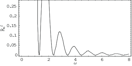
Figure 1: Square of eigenfunction at the horizon with respect to $\omega$

Eigenvalues for the Neumann boundary condition at the horizon are between those for the Dirichlet boundary condition.

4.1 The Dirichlet boundary condition at the horizon

We study the eigenvalue map with the eigenvalue points in $(m,\omega)$ plane for the Dirichlet boundary condition at the horizon.

4.1.1 The eigenvalue of no black hole rotation

In the case of no black hole rotation $J=0$, the eigenvalue points $\omega_{n}$ for each fixed $n$ is shown in Fig.2. Parameters are those of Eq.(21). In the map, each eigenvalue point $(\omega_{n},n=0,1,\dots)$ forms a convex curve with respect to the horizontal line. In this $J=0$ case, the eigenvalue equation Eq.(16) is invariant under the transformation $\omega\rightarrow\omega,m\rightarrow-m$ , which means that the eigenvalue $\omega_{n}$ is the even function of $m$. This is the origin of the convexity of the curve in $J=0$ case.

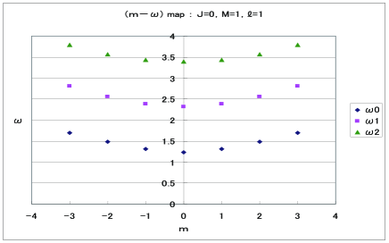
Figure 2: The eigenvalue map of no rotation for the Dirichlet B.C.

4.1.2 The scalar mass effect

For the Dirichlet boundary condition, the scalar field mass effect ($\mu\neq 0$) is studied in Fig.3 with parameter values

$$M=1,\ J=0,\ \ell=1,\ \mu=1\ .$$ (23)

We see from the map that the effect of the scalar mass term is to uniformly shift each eigenvalue to the larger value and the qualitative feature is similar to the massless case $(\mu=0)$.

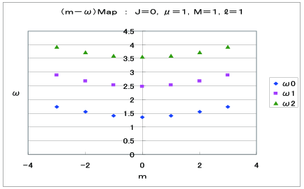
Figure 3: The scalar mass effect( $\mu=1$) of no rotation

4.1.3 The rotation effect of the black hole

Next, for the Dirichlet boundary condition, we study the rotation effect of the black hole to the eigenvalue $(m,\omega)$ with parameters

$$M=1,\ J=0.2,\ \mu=0,\ \ell=1\ .$$ (24)

We can see in Fig. 4 that points of eigenvalues $(m,\omega)$ rotate corresponding to the angler velocity $\Omega_{\rm H}$ in case of $J=0.2$ compared with the case of $J=0$ (See Fig. 2).

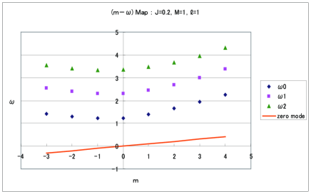
Figure 4: Rotation effect of black hole for Dirichlet B.C.

The zero mode line, which is defined:

$$\omega-\Omega_{\rm H}m=0\ \ {\mbox{\rm with}}\ \ -\infty<m<\infty\ ,$$ (25)

is also shown in Fig.4. We notice that all points of eigenvalues lie in the physical region $0<\omega-\Omega_{\rm H}m$.

4.2 The Neumann boundary condition at the horizon

For the Neumann boundary condition at horizon, we study the eigenvalue map with eigenvalue points in $(m,\omega)$ plane.

4.2.1 The eigenvalue of no black hole rotation

In case of no black hole rotation, the eigenvalue points $\omega_{n}$ for each fixed $n$ is shown in Fig.5 with same parameter values as those in Eq.(7). For the Neumann boundary condition, each eigenvalue with fixed principal quantum number $n$ and azimuthal quantum number $m$ in Fig.5 exist between the corresponding value of that for the Dirichlet boundary condition (See Fig.2). We see that the ground state eigenvalues $\omega_{0}$ of $n=0$ for the Neumann boundary condition is lower than that for the Dirichlet boundary condition because it has no node.

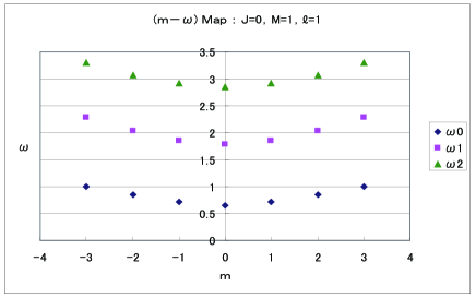
Figure 5: The eigenvalue map of no rotation for the Neumann B.C.

4.2.2 The rotation effect of the black hole

For the Neumann boundary condition, we study the rotation effect of the black hole to points of eigenvalues $(m,\omega)$ with parameter values

$$M=1,\ J=0.2,\ \mu=0,\ \ell=1\ .$$ (26)

We can see from the Fig.6 that points of eigenvalues $(m,\omega)$ rotate corresponding to the angler velocity $\Omega_{\rm H}$ in case of $J=0.2$ compared with no black hole rotation case in Fig.5 as in the case of the Dirichlet boundary condition.

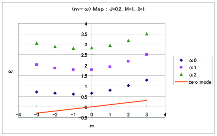
Figure 6: Rotation effect of black hole for the Neumann B.C.

The zero mode line separate all the eigenvalue region into two parts: one is the allowed physical region $0<\omega-\Omega_{\rm H}m$ with $-\infty<m<\infty$ and another is the unphysical region $0>\omega-\Omega_{\rm H}m$ with $-\infty<m<\infty$.

5 Summary and discussion

We have studied the eigenvalue problem of scalar fields in the BTZ black hole spacetime. We imposed the Dirichlet boundary condition at infinity and the Dirichlet or the Neumann boundary condition at the horizon and found the explicit form of eigenfunctions and eigenvalues. The main results are summarized in the following.

• Eigenvalue equations in Eq.(16) and Eq.(18) are derived. Eigenvalues for normal modes $\omega$ are characterized by the principal quantum number $n\ (n=0,1,2,\dots)$ and the azimuthal quantum number $m\ (-\infty,\dots,-1,0,1,2,\dots\infty)$. The eigenfunction $R_{\infty}$ in Eq. (9) is determined with boundary condition and all eigenvalues and eigenfunctions are determined.

• The set of eigenvalues $(\omega,m)$ forms a convex curves in $(\omega,m)$ plane for fixed $n$. For the Dirichlet boundary condition, we showed the convexity property of no black hole rotation, but this convexity property holds for other cases too.

• The scalar mass effect is to uniformly shift each eigenvalue to the larger value but the qualitative feature is similar to the massless case $(\mu=0)$.

• Points of eigenvalues $(\omega,m)$ rotate corresponding to the angular velocity $\Omega_{\rm H}$ for both the Dirichlet and the Neumann boundary conditions. Then the allowed physical eigenvalue region of $0<\omega$ for $J=0$ becomes $0<\omega-\Omega_{\rm H}m$ for $J>0$. This result indicates that the super-radiant instability [17, 18, 19, 20] doesn’t occur in the (2+1)-dimensional BTZ black hole spacetime.

The explicit construction of eigenvalues and eigenfunctions studied in this paper plays the complimentary role with the general consideration of our previous paper [24]. Our method will be extend to the (3+1)-dimensional and more higher dimensional cases [25].

References

- [1] The 17th Workshop on General Relativity and Gravitation in Japan, at Nagoya University, Nagoya, Japan, on December 3 - 7, 2007.
- [2] N.D. Birrell and P.C.W. Davies, “Quantum Fields in Curved Space”, Cambridge University Press (1982).
- [3] J.D. Bekenstein, Phys. Rev. D7 (1973) 2333.
- [4] M. Bardeen, B. Carter and S.W. Hawking, Comm. Math. Phys. 31 (1973) 161.
- [5] S.W. Hawking, Comm. Math. Phys.43 (1975) 199.
- [6] G. ’t Hooft, Nucl. Phys. B256 (1985) 727.
- [7] J.M. Bardeen, W.H. Press and S.A. Teukolsky, Astrophys. J. 178 (1972) 347; S.A. Teukolsky and W.H. Press, Astrophys. J. 193 (1974) 443; W.H. Press and S.A. Teukolsky, Nature 238 (1972) 211.
- [8] V. Cardoso, Ó.J.C. Dias, J.P.S. Lemos and S. Yoshida, Phys.Rev. D70 (2004) 044039.
- [9] S. Mukohyama, Phys. Rev. D61 (2000) 124021.
- [10] M. Bañados, C. Teitelboim and J. Zanelli, Phys. Rev. Lett. 69 (1992) 1849.
- [11] D. Birmingham, Phys.Rev. D64 (2001) 064024.
- [12] V. Cardoso and J.P.S. Lemos, Phys.Rev. D63 (2001) 124015.
- [13] S. Carlip, “Conformal Field Theory, (2+1)-Dimensional Gravity, and the BTZ Black Hole”, gr-qc/0503022.
- [14] K.S. Gupta and S. Sen, Phys. Lett. B646 (2007), 265.
- [15] E. Witten, “Three-Dimensional Gravity Reconsidered”, arXiv:0706.3359.
- [16] R.K. Gupta and A. Sen, “Consistent Truncation to Three Dimensional (Super-) gravity”, arXiv:0710.4177.
- [17] I. Ichinose and Y. Satoh, Nucl. Phys. 447 (1995) 340.
- [18] S.-W. Kim, W.T. Kim, Y.-J. Park and H. Shin, Phys. Lett. B392 (1997) 311.
- [19] L. Fatibene, M. Ferraris, M. Fracaviglia and M. Raiteri, Phys. Rev. D60 (1999) 124012.
- [20] J. Ho and G. Kang, Phys. Lett. B445 (1998) 27.
- [21] D. Birmingham and S. Mokhatari, arXiv:0709.2388.
- [22] A. Ishibashi and H. Kodama, Prog. Theor. Phys. 111 (2004) 29.
- [23] H. Kodama, J. Korean Phys. Soc. 45 (2004) S68.
- [24] M. Kenmoku, M. Kuwata and K. Shigemoto, arXive:0801.2044.
- [25] M. Kenmoku, M. Kuwata and K. Shigemoto, in preparation (2008).