Instabilities of chromodyons in SO(5) gauge theory

Abstract

Attempts to construct chromodyons — objects with both magnetic charge and non-Abelian electric charge — in the context of spontaneously broken gauge theories have been thwarted in the past by topological obstructions to globally defining the unbroken non-Abelian “color” subgroup. In this paper we consider the possibility of chromodyons in a theory with SO(5) broken to ${\rm SU(2)}\times{\rm U(1)}$, where the topological obstructions are absent. We start by constructing a monopole with only magnetic charge. By exciting a global gauge zero mode about this monopole, we obtain a chromodyonic configuration that is an approximate solution of the field equations. We then numerically simulate the time evolution of this initial state, to see if it settles down in a stationary solution. Instead, we find that chromo-electric charge is continually radiated away, with every indication that this process will continue until this charge has been completely lost. We argue that this presents strong evidence against the existence of stable chromodyons.

I Introduction

The magnetic monopoles that arise in spontaneously broken gauge theories can easily be generalized to dyons that have a U(1) electric charge in addition to their magnetic charge. It then is natural to ask whether, in cases where the unbroken symmetry is non-Abelian, it is possible to have monopoles carrying non-Abelian electric charge. Such objects, referred to as chromodyons, were first considered in the context of an SU(5) grand unified theory. After attempts to construct such chromodyons failed Abouelsaood:1982dz , it was shown that the non-Abelian magnetic charge of the SU(5) monopole creates a topological obstruction to the existence of non-Abelian “color” electric charge Nelson:1983bu ; Balachandran:1982gt ; Balachandran:1983xz ; Balachandran:1983fg ; Horvathy:1985bp ; Horvathy:1984yg , and the issue was abandoned for a number of years. Since then, however, it has been realized that, with other choices of gauge group, there can be monopoles with purely Abelian magnetic charge, even though the unbroken gauge group is non-Abelian Weinberg:1982jh . Because there is then no topological barrier to a color electric charge, it is natural to revisit the subject and consider whether chromodyons can exist.

Let us first recall how ordinary U(1) dyons arise. When there is an unbroken U(1) symmetry, any soliton with a nonvanishing charged field has a zero mode corresponding to a shift in the phases of the complex charged fields. Exciting this mode in a time-dependent fashion produces a U(1) charge. If the U(1) symmetry is gauged, it may be possible to gauge transform away the time-dependence of the phase, but the gauge-invariant electric charge remains. The simplest example of this occurs with SU(2) broken to U(1), where the Julia-Zee dyon Julia:1975ff arises from rotation of the phase of the massive vector boson fields in the core of the ’t Hooft-Polyakov monopole 't Hooft:1974qc ; Polyakov:1974ek .

Similarly, if there is an unbroken non-Abelian symmetry, excitation of the gauge orientation zero modes of a soliton gives rise to a non-Abelian electric charge. In the theory with SU(5) broken to ${\rm SU(3)}_{\rm color}\times{\rm U(1)}_{\rm EM}$, the unit monopoles have nontrivial fields that are not invariant under the unbroken SU(3). Hence, one would expect to be able to generate dyons that were charged under the color SU(3) (hence the term “chromodyon”) by exciting the resulting global gauge zero modes. However, Abouelsaood Abouelsaood:1982dz found that, because the gauge potential has a $1/r$ tail in the unbroken subgroup, some of the expected zero modes are non-normalizable, and the proposed construction does not go through. A deeper explanation for this was given by Nelson and Manohar Nelson:1983bu , and by Balachandran et al. Balachandran:1982gt ; Balachandran:1983xz ; Balachandran:1983fg , who showed that the non-Abelian Coulomb magnetic field creates a topological obstruction that prevents one from globally defining a basis for the unbroken color subgroup. This inability to define “global color” is the fundamental reason for the nonexistence of the SU(5) chromodyons.

These barriers to the existence of a chromodyon would both be absent if the total magnetic charge were purely Abelian. This can certainly be achieved by assembling a collection of magnetic monopoles such that the non-Abelian components of their charges sum to zero; a two-monopole example of this was studied by Coleman and Nelson Nelson:1983fn . However, what we need to produce a chromodyon is a single monopole with purely Abelian magnetic charge. While there are no such monopoles in the SU(5) theory, they do exist in a theory with SO(5) broken to U(1)$\times$SU(2). These were first discovered Weinberg:1982jh in the BPS limit, where they appear as spherically symmetric classical solutions that are characterized by a “cloud size” $b$ that can take on any positive value. These can be interpreted as being composed of a massive monopole, carrying both Abelian and non-Abelian magnetic charge, and a massless monopole, with only non-Abelian magnetic charge. At the semiclassical level, the latter is manifested as a cloud of non-Abelian field, of radius $b$, that surrounds the core of the massive monopole and completely shields the non-Abelian part of its magnetic charge. In the BPS limit the energy is independent of $b$. However, if the Lagrangian includes a nonvanishing potential, the cloud size is no longer arbitrary, but rather is fixed. This then gives a magnetic monopole whose long-range field lies only in the U(1) sector, but whose core transforms under the unbroken SU(2) and thus gives rise to the gauge zero modes from which we might hope to construct a chromodyon. It is this system that we will study.

We start, in Sec. II, by constructing the static SO(5) monopole. An analytic solution exists for the BPS case. However, as we explain later on, the possibility of varying the cloud size makes these unsuitable for our purposes. Instead, we must take for our starting point a non-BPS monopole, for which the field equations must be solved numerically. Then, in Sec. III, we construct a chromodyonic configuration from this monopole by applying an SU(2) gauge rotation and solving for the $A_{0}$ field that is required by Gauss’s law. Although this is not an exact static solution of the field equations, one might expect it to be close to the desired chromodyon. We test this by numerically simulating the time evolution with this as the initial configuration. We describe the details of this simulation in Sec. IV. The results are described in Sec. V. We find that, rather than evolving toward a stable chromodyon, the chromodyonic configuration continually radiates non-Abelian charge. Although we are not able to continue the simulation long enough to verify that this charge is completely radiated away, every evidence indicates that this will be the case. Our conclusions are summarized in Sec. VI. There are two Appendices containing some technical details.

II SO(5) monopoles

We are interested in theories with Lagrangian densities of the form

$${\cal L}=-{1\over 4}{\rm Tr\,}F^{\mu\nu}F_{\mu\nu}-{1\over 2}{\rm Tr\,}D^{\mu}\Phi\,D_{\mu}\Phi-V(\Phi)\,.$$ (1)

Here the gauge field $A_{\mu}$ and the adjoint representation Higgs field $\Phi$ are both written as imaginary antisymmetric $5\times 5$ matrices.

To describe the components of these and other adjoint representation fields, we will adopt the following conventions. In the defining representation, the generators of SO(5) are the ten 5$\times$5 matrices

$$(J^{mn})_{ij}=-i(\delta_{im}\delta_{jn}-\delta_{in}\delta_{jm})\,,\qquad 1\leq m<n\leq 5\,.$$ (2)

From these we can define six matrices

$$h_{a}={1\over 2}\left({1\over 2}\epsilon_{abc}J^{bc}+J^{a4}\right)\,,\qquad k_{a}={1\over 2}\left({1\over 2}\epsilon_{abc}J^{bc}-J^{a4}\right)$$ (3)

that generate SO(4)=SU(2)$\times$SU(2). We can then decompose any adjoint representation field $P$ in terms of two triplets, $P_{(1)}^{a}$ and $P_{(2)}^{a}$, and $P_{(3)}^{\mu}$ ($\mu=1,2,3,4$) via

$$P={\bf P}_{(1)}{\bf\cdot h}+{\bf P}_{(2)}{\bf\cdot k}+P_{(3)}^{\mu}J^{\mu 5}\,.$$ (4)

We will refer to $P_{(1)}$, $P_{(2)}$, and $P_{(3)}$ as the first-, second-, and third-sector components, respectively.

SO(5) can be broken to SU(2)$\times$U(1) in two inequivalent ways. In the first, corresponding to the decomposition ${\rm SO(5)}\supset{\rm SO(3)}\times{\rm SO(2)}$, the SU(2) is the subgroup, with the generators $J^{ab}=\epsilon_{abc}(h_{c}+k_{c})$, that rotates the first three components of a five-vector among themselves. We will be concerned with the second possibility, in which the unbroken SU(2) is one of the factors of the ${\rm SO}(4)={\rm SU(2)}\times{\rm SU(2)}$ subgroup that mixes the first four components of a five-vector among themselves; we will choose it to be the subgroup generated by the $k_{a}$.

We will be seeking spherically symmetric monopole solutions. If we also require that the fields have positive parity, the most general spherically symmetric ansatz can be written as

$$A^{a}_{i(1)}=\epsilon_{aim}{\hat{r}}_{m}A(r)\,, \quad\quad\Phi^{a}_{(1)}={\hat{r}}_{a}H(r)\,,\hskip 57.81621pt$$ (5)

$$A^{a}_{i(2)}=\epsilon_{aim}{\hat{r}}_{m}G(r)\,, \quad\quad\Phi^{a}_{(2)}={\hat{r}}_{a}K(r)\,,$$ (6)

$$A_{i(3)}^{\mu}=\sqrt{2}\left[\delta^{i\mu}\,F(r)+\delta^{\mu a}{\hat{r}}_{i}{\hat{r}}_{a}S(r)\right]\,, \quad\quad\Phi^{\mu}_{(3)}=-\sqrt{2}\,\delta^{4\mu}J(r)\,,$$ (7)

where Latin indices run from 1 to 3 and $\mu$ runs from 1 to 4.

Actually, there is some redundancy in this ansatz. A gauge transformation of the form

$$\Lambda_{S}=e^{i\psi(r)\hat{r}^{a}J^{a5}}$$ (8)

preserves the ansatz, but with new coefficient functions, which we indicate with a tilde, given by

$$\tilde{H}+\tilde{K} = H+K\,,$$ (9)

$$\tilde{H}-\tilde{K} = (H-K)\cos\psi+2\sqrt{2}J\sin\psi\,,$$ (10)

$$2\sqrt{2}\tilde{J} = -(H-K)\sin\psi+2\sqrt{2}J\cos\psi\,,$$ (11)

$$\tilde{A}-\tilde{G} = A-G\,,$$ (12)

$$\tilde{A}+\tilde{G}+{2\over er} = \left(A+G+{2\over er}\right)\cos\psi+2\sqrt{2}F\sin\psi\,,$$ (13)

$$2\sqrt{2}\tilde{F} = -\left(A+G+{2\over er}\right)\sin\psi+2\sqrt{2}F\cos\psi\,,$$ (14)

$$\tilde{S} = S+F(1-\cos\psi)+{1\over 2\sqrt{2}}\left(A+G+{2\over er}\right)\sin\psi-{1\over\sqrt{2}\,e}{d\psi\over dr}\,.$$ (15)

From the last of these equations, we see that $S(r)$ can always be gauged away with a suitable choice of $\psi(r)$. We will henceforth assume that this has been done, so that $S(r)$ vanishes identically.

Requiring that the fields be nonsingular at the origin gives the boundary conditions

$$A(0)=G(0)=H(0)=K(0)=0\,.$$ (16)

The functions $F$ and $J$ can be nonzero at the origin. However, examination of the field equations, which we will display below, shows that nonsingular solutions must have

$$F^{\prime}(0)=J^{\prime}(0)=0\,,$$ (17)

where a prime denotes differentiation with respect to $r$.

To obtain the symmetry breaking that we want, the asymptotic value of the Higgs field must lie in the subgroup generated by the $h_{a}$, giving the boundary conditions

$$H(\infty)=v\,,\qquad K(\infty)=J(\infty)=0\,.$$ (18)

With this choice, the third-sector gauge fields are massive, so $F(r)$ falls exponentially fast at large distance. The behavior of the other, massless, gauge fields depends on the magnetic charge. If the latter is a purely Abelian unit charge, then at large distance

$$A(r)\sim-1/er\,,\qquad G(r)\mathrel{\mathchoice{\lower 3.0pt\vbox{\halign{$\m@th\displaystyle\hfill#\hfil$\cr<\crcr\sim\crcr}}}{\lower 3.0pt\vbox{\halign{$\m@th\textstyle\hfill#\hfil$\cr<\crcr\sim\crcr}}}{\lower 3.0pt\vbox{\halign{$\m@th\scriptstyle\hfill#\hfil$\cr<\crcr\sim\crcr}}}{\lower 3.0pt\vbox{\halign{$\m@th\scriptscriptstyle\hfill#\hfil$\cr<\crcr\sim\crcr}}}}{\rm const}/r^{2}\,,\qquad F(r)\sim e^{-evr/2}\,.$$ (19)

In Ref. Weinberg:1982jh it was shown that in the BPS limit of vanishing scalar potential there is a solution given by

$$A(r)={v\over\sinh evr}-\frac{1}{er}\,,$$ (20)

(21)

$$H(r)=v\,\coth evr-\frac{1}{er}\,,$$ (22)

(23)

$$G(r)=K(r)=\left({v\over\sinh evr}-{1\over er}\right)\,L(r;b)\,,$$ (24)

(25)

$$F(r)=-J(r)={v\over\sqrt{8}\,\cosh(evr/2)}\,\sqrt{L(r;b)}\,,$$ (26)

(27)

$$S(r)=0\,,$$ (28)

where $b$ is any positive real number and

$$L(r;b)=\frac{b}{b+r\,\coth(evr/2)}\,.$$ (29)

This solution can be interpreted as being composed of two distinct fundamental monopoles. One is a massive monopole, with core radius $\sim 1/ev$, whose magnetic charge has both non-Abelian and Abelian components. The other is a massless monopole that is manifested at the semiclassical level as a cloud of radius $b$ whose magnetic charge cancels the non-Abelian part of the massive monopole’s charge. This can be seen by computing the large distance behavior of the magnetic field. For $1/ev\ll r\ll b$, both $A(r)$ and $G(r)$ fall as $1/r$, and so

$$B_{i(1)}^{a}={{\hat{r}_{a}}{\hat{r}_{i}}\over er^{2}}+O(1/r^{3})\,,$$ (30)

$$B_{i(2)}^{a}={{\hat{r}_{a}}{\hat{r}_{i}}\over er^{2}}+O(1/r^{3})\,.$$ (31)

(The third-sector fields fall exponentially outside the massive monopole core and play no role here.) Outside the massless cloud, $r\gg b$, $G(r)\sim-b/er^{2}$. As a result, $B_{i(2)}^{a}$ falls faster than $1/r^{2}$, while $B_{i(1)}^{a}$ is unchanged. Hence, the long-range magnetic field, and thus the total magnetic charge, have only first-sector components and are purely Abelian.

One might think that the knowledge of the explicit analytic form of this monopole solution would make it an ideal case for constructing chromodyons. As we will see in the next section, this turns out not to be so. The difficulty arises from the fact that the energy of the BPS monopole is independent of the cloud size $b$, so that a small perturbation can cause the cloud to expand without bound. To avoid this problem, we will add a potential term that effectively fixes the cloud size. With this term included, the BPS limit no longer applies, so we will have to solve the full set of second-order field equations. Because this cannot be done analytically, we will resort to numerical solution.

Thus, let us add a potential of the form

$$V(\Phi)=-{\mu^{2}\over 2}\leavevmode\hbox{Tr}\,\Phi^{2}+a(\leavevmode\hbox{Tr}\,\Phi^{2})^{2}+b\leavevmode\hbox{Tr}\,\Phi^{4}$$ (32)

where $\mu$, $a$, and $b$ are constants. In order to obtain the desired symmetry breaking, $b$ must be positive, while the requirement that the potential be bounded from below gives the condition $4a+b>0$. At the minimum of the potential,

$$\leavevmode\hbox{Tr}\,\Phi^{2}\equiv v^{2}={\mu^{2}\over 4a+b}\,.$$ (33)

There is an SU(2) singlet Higgs scalar with mass

$$m_{s}=\sqrt{2}\,\mu$$ (34)

and an SU(2) triplet with mass

$$m_{t}=\sqrt{2(1-c)}\,\mu\,,$$ (35)

where

$$c\equiv{4a\over 4a+b}\,.$$ (36)

The positivity of $b$ implies that $-\infty<c<1$, with the two limits corresponding to $m_{s}\ll m_{t}$ and $m_{t}\ll m_{s}$, respectively.

Substitution of our spherically symmetric ansatz, Eq. (7), into the Euler-Lagrange equations,

$$D_{j}F^{ji} = ie[\Phi,D^{i}\Phi],$$

$$D_{j}D^{j}\Phi = {\partial V\over\partial\Phi}\,,$$ (37)

yields seven ordinary differential equations (ODEs), corresponding to the seven coefficient functions in our ansatz. Note that even though we can use the gauge freedom described by Eqs. (8) and (15) to make $S(r)$ identically zero, there is still a corresponding ODE. However, while the other six ODEs are second order, this last is a constraint equation relating the coefficient functions and their first derivatives. If we set $S=0$, this equation, which we will refer to as the $S$ constraint, takes the form

$$0 = \left(A+G+{2\over er}\right)F^{\prime}-\left(A^{\prime}+G^{\prime}-{2\over er^{2}}\right)F+{1\over 2}(H-K)J^{\prime}-{1\over 2}(H^{\prime}-K^{\prime})J$$ (39)

$$-e\left[{1\over 2}\left(A+G+{2\over er}\right)^{2}+{1\over 4}(H-K)^{2}+2J^{2}+4F^{2}\right]F$$

while the other six ODEs become

$$A^{\prime\prime} = -\frac{2}{r}A^{\prime}+\frac{2}{r^{2}}A+6eFF^{\prime}+\frac{3e}{r}A^{2}+\frac{e}{r}H^{2}$$ (41)

$$+e^{2}\left(A^{3}+AH^{2}+AJ^{2}+5AF^{2}-GF^{2}-GJ^{2}+3HFJ+KFJ\right)\,,$$

$$G^{\prime\prime} = -\frac{2}{r}G^{\prime}+\frac{2}{r^{2}}G-6eFF^{\prime}+\frac{3e}{r}G^{2}+\frac{e}{r}K^{2}$$ (44)

$$+e^{2}\left(G^{3}+GK^{2}+GJ^{2}+5GF^{2}-AF^{2}-AJ^{2}-3KFJ-HFJ\right)\,,$$

$$F^{\prime\prime} = -\frac{1}{r}F^{\prime}+\frac{e}{2}(A+G)F^{\prime}+e(A^{\prime}+G^{\prime})F+\frac{2e}{r}(A+G)F+\frac{e}{2r}(H-K)J$$ (48)

$$+e^{2}\left(4F^{2}+A^{2}+G^{2}+\frac{1}{4}H^{2}+\frac{1}{4}K^{2}+2J^{2}+\frac{1}{2}HK-AG\right)F$$

$$+\frac{e^{2}}{4}(3AH-3GK-GH+AK)J\,,$$

$$H^{\prime\prime} = -\frac{2}{r}H^{\prime}+\frac{2}{r^{2}}H-4eFJ^{\prime}-2eF^{\prime}J+\frac{4e}{r}AH$$ (52)

$$+e^{2}\left(3F^{2}H+F^{2}K+2A^{2}H+6AFJ-2FGJ\right)$$

$$+{\mu^{2}\over v^{2}}\left[H(H^{2}+3K^{2}-v^{2})+4J^{2}(H-K)+c(4J^{2}K-2HK^{2})\right]\,,$$

$$K^{\prime\prime} = -\frac{2}{r}K^{\prime}+\frac{2}{r^{2}}K+4eFJ^{\prime}+2eF^{\prime}J+\frac{4e}{r}GK+$$ (56)

$$+e^{2}\left(2G^{2}K+3F^{2}K+F^{2}H+2AFJ-6GFJ\right)$$

$$+{\mu^{2}\over v^{2}}\left[K(K^{2}+3H^{2}-v^{2})+4J^{2}(K-H)-c(2H^{2}K-4J^{2}H)\right]\,,$$

$$J^{\prime\prime} = -\frac{2}{r}J^{\prime}+\frac{e}{2}HF^{\prime}-\frac{e}{2}KF^{\prime}+eH^{\prime}F-eK^{\prime}F+\frac{2e}{r}HF-\frac{2e}{r}KF$$ (60)

$$+{e^{2}\over 2}\left(A^{2}+G^{2}+12F^{2}-2AG\right)J+{e^{2}\over 2}\left(3AH-3GK+AK-GH\right)F$$

$$+{\mu^{2}\over v^{2}}\left[8J^{2}+(H-K)^{2}-v^{2}+c(2HK-4J^{2})\right]J\,.$$

These equations are not all independent. For example, the $F^{\prime\prime}$ equation can be derived from the $S$ constraint and the other five ODEs. The converse is not quite true, because there are solutions of the six second-order equations that do not satisfy the $S$ constraint. However, if the $S$ constraint holds at one value of $r$, the remaining ODEs imply that it holds for all $r$. In particular, the $S$ constraint is satisfied for all $r$ if the fields at spatial infinity obey Eqs. (18) and (19).

In the BPS case, the exponential approach of the coefficient functions to their asymptotic behavior is governed by a single mass scale, $ev$. With the potential added, three different mass scales — $ev$, $m_{s}$, and $m_{t}$ — come into play. To simplify our numerical simulations of the time evolution and to avoid the well-known stiffness problem, we want these characteristic lengths to be close to each other. To that end we set $\mu=ev$ and $c=0.5$, so that $ev=m_{t}=m_{s}/\sqrt{2}$.

We choose to numerically solve the six ODEs in Eq. (60) and then check the solution against the $S$ constraint. We use a MATLAB package – SBVP 1.0 sbvp – to solve this boundary value problem. By using the collocation method, the SBVP numerical package can handle the singular terms in Eq. (60) with high accuracy near the origin, where $r\rightarrow 0$. Our numerical solution is shown in Fig. 1. The $S$ constraint has been checked to be automatically satisfied within the numerical error.

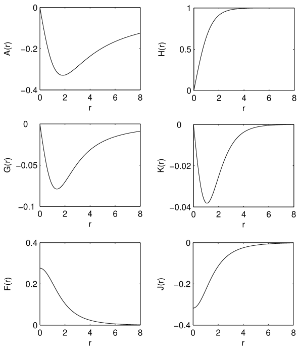
Figure 1: Monopole solution in the non-BPS SO(5) gauge theory. The radial distance $r$ is given in units of $1/ev$, and the coefficient functions in units of $v$.

It should be noted that this solution is not unique. Setting $G=F=J=K=0$ reduces the field equations to two coupled equations for $A$ and $H$ that are identical to those of the SU(2) theory. This then yields a solution that is simply an embedding of the SU(2) unit monopole via the subgroup generated by the $h_{a}$. For our choice of parameters, the mass of this pure SU(2) solution is $1.287M_{\rm BPS}$, where $M_{\rm BPS}=4\pi v/e$ is the mass of the unit BPS monopole. By contrast, the non-embedding solution shown in Fig. 1 has a mass of $1.253M_{\rm BPS}$. Note that the mass difference is numerically significant, well above the numerical errors.

III Constructing a chromodyonic configuration

In a U(1) dyonic soliton the electric charge results from a time-dependent phase of a complex field. In a similar fashion, a magnetically charged configuration with a time-dependent orientation with respect to a non-Abelian group carries non-Abelian electric charge and is a chromodyon. In this section we will show how such chromodyons can be constructed from time-independent solutions such as those obtained in the previous section. We start with a static solution $\{(A_{i})_{\rm static}({\bf r})$, $(\Phi)_{\rm static}({\bf r})\}$. As our first step, we excite one of the zero modes of the static solution and uniformly rotate its SU(2) orientation to obtain

$$(A_{i})_{\rm I} = R(t)\,(A_{i})_{\rm static}R^{-1}(t)\,,$$

$$(\Phi)_{\rm I} = R(t)(\Phi)_{\rm static}R^{-1}(t)\,,$$ (1)

where

$$R(t)=e^{i\,k_{3}\omega_{0}t}$$ (2)

and the generator $k_{3}$ is defined in Eq. (3). It is critical to realize that this is not a gauge transformation, because the latter would have required that we also add a spatially constant $A_{0}=-(\omega_{0}/e)k_{3}$. However, we do need a nonzero $A_{0}$ in order to satisfy the Gauss’s law constraint

$$D_{j}F^{j0}=ie[\Phi,D^{0}\Phi]\,.$$ (3)

Solving this equation, given $(A_{i})_{\rm I}$ and $(\Phi)_{\rm I}$ and the boundary condition

$$A_{0}(\infty)=0\,,$$ (4)

yields a solution that we denote by $(A_{0})_{\rm II}$. This gives us a time-dependent configuration $\{(A_{0})_{\rm II},(A_{i})_{\rm I},(\Phi)_{\rm I}\}$.

It is often more convenient to work instead with the stationary configuration obtained by applying a gauge transformation with gauge function $\Lambda=R^{-1}$. This gives us $\{(A_{0})_{\rm III},(A_{i})_{\rm static},(\Phi)_{\rm static}\}$ where

$$(A_{0})_{\rm III}={\omega_{0}\over e}\,k_{3}+R^{-1}(A_{0})_{\rm II}R\,.$$ (5)

It is not hard to see that we could have obtained this final configuration by directly solving Gauss’s law with $(A_{i})_{\rm static}$ and $(\Phi)_{\rm static}$ given and $A_{0}$ obeying a different boundary condition,

$$A_{0}(\infty)={\omega_{0}\over e}\,k_{3}\,.$$ (6)

We denote the solution of this equation as $(A_{0})_{\rm static}$.

Even when working in this static gauge, it is convenient to describe the extra energy associated with this configuration in rotational terms. The relevant “moment of inertia” is given by the spatial integral of the sum of the squares of the field components that undergo the phase rotation. Since the characteristic length scale is $\sim(ev)^{-1}$, while the natural scale of the fields is $v$, we have

$$E_{\rm ch}\sim I\omega_{0}^{2}\sim\left({1\over ev}\right)^{3}v^{2}\omega_{0}^{2}\sim{v\over e}\left({\omega_{0}\over ev}\right)^{2}\,.$$ (7)

Similarly, the SU(2) electric charge has a magnitude

$$q_{E}\sim eI\omega_{0}\sim{1\over e}\left({\omega_{0}\over ev}\right)$$ (8)

with the extra factor of $e$ arising because the electric charge is $e$ times the momentum conjugate to the phase rotation.

The configuration $\{(A_{0})_{\rm static},(A_{i})_{\rm static},(\Phi)_{\rm static}\}$ has both a U(1) magnetic charge and an SU(2) electric charge, and so is a chromodyon. The question that we need to address is whether it is a solution of the field equations. It is easy to see that it cannot be, because the rotation in group space induces a deformation of the field profiles, just as the spatial rotation of a solid object induces a deformation of its shape. However, this deformation is of order $\omega_{0}^{2}$, and so should require only a small modification of the configuration if $\omega_{0}$ is sufficiently small. If this is the only correction needed, then the theory does indeed have a stable static chromodyon solution. On the other hand, it may be that there is no such static solution. We will test for this possibility by taking $\{(A_{0})_{\rm static},(A_{i})_{\rm static},(\Phi)_{\rm static}\}$ as an initial condition and then letting the fields evolve in time according to the field equations. If the deformation resulting from the rotation in SU(2) space is the only impediment to its being a static solution, the fields should oscillate, with an initial amplitude proportional to $\omega_{0}^{2}$, and eventually settle down in the true static solution.

In order to do this, we need to determine $(A_{0})_{\rm static}$. Thus, our immediate task is to solve Eq. (3) subject to the boundary condition that $A_{0}(\infty)=(\omega_{0}/e)k_{3}$. The fields $(A_{i})_{\rm static}$ and $(\Phi)_{\rm static}$ are both spherically symmetric. However, the boundary condition on $A_{0}$ breaks this symmetry, so we can only assume that $A_{0}$ has an axial symmetry. The most general ansatz for $A_{0}$ is then

$$A_{0(1)}^{a}={\hat{r}}^{a}u(\rho,z)\,,\qquad\quad A_{0(1)}^{3}=w(\rho,z)\,,$$ (10)

$$A_{0(2)}^{a}={\hat{r}}^{a}b(\rho,z)\,,\,\qquad\quad A_{0(2)}^{3}=Q(\rho,z)\,,$$ (11)

$$A_{0(3)}^{a}=\sqrt{2}\,\epsilon_{ab}{\hat{r}}^{b}q(\rho,z)\,,\quad\quad A_{0(3)}^{3}=0\,,$$ (12)

$$A_{0(3)}^{4}=-\sqrt{2}\,t(\rho,z)\,,$$ (13)

where $a$ and $b$ are either 1 or 2 and $\rho=\sqrt{x^{2}+y^{2}}$. The boundary conditions at spatial infinity require that $Q$ approach $\omega_{0}/e$ and that the other coefficient functions tend to zero.

Substituting this ansatz into Gauss’s law, Eq. (3), yields the set of second-order partial differential equations that are displayed in Appendix A. These rather complicated equations experience a remarkable simplification if $(A_{i})_{\rm static}$ and $(\Phi)_{\rm static}$ are taken to be the BPS solution of Eq. (28). In this case, they can be satisfied by setting all the coefficient functions except $Q$ to zero, taking $Q(\rho,z)=Q(r)$, and requiring that

$$\frac{dQ(r)}{dr}+eG(r)Q(r)=0\,,$$ (14)

where $G(r)$ is the second-sector gauge field function given in Eq. (28). The solution to Eq. (14) is

$$Q(r)={\omega_{0}\,b\over eL(r,b)}\,{\partial L(r,b)\over\partial b}=\left({\omega_{0}\over e}\right)\frac{r\,\leavevmode\hbox{coth}(evr/2)}{b+r\,\leavevmode\hbox{coth}(evr/2)}\,.$$ (15)

Unfortunately, this simple solution turns out not to be useful. To see this, recall that for small velocities the dominant time dependence of a soliton arises entirely through excitation of its zero modes, whose dynamics is governed by the moduli space Lagrangian. For the generic case, with a nonzero scalar field potential, there are seven zero modes about $\{(A_{i})_{\rm static},(\Phi)_{\rm static}\}$. Four of these — three translation modes and one U(1) phase mode — are irrelevant for our purposes. The remaining three are SU(2) orientation modes, one of which has been excited by the transformation in Eq. (1). Within the moduli space approximation (MSA) there would be uniform motion in the corresponding collective coordinate. In the gauge where $A_{0}(\infty)=0$, the soliton would rotate uniformly in SU(2) space, as described by Eq. (1).

In the BPS case there is an additional zero mode, corresponding to the freedom to vary the cloud radius $b$. The moduli space Lagrangian governing the eight zero modes is given by

$$L_{\rm MS}={1\over 2}M\,\dot{\bf X}^{2}+{1\over 2M}\dot{\chi}^{2}+{1\over 2}\left\{{\dot{b}^{2}\over b}+b\left[\dot{\alpha}^{2}+\sin^{2}\alpha\>\>\dot{\beta}^{2}+(\dot{\gamma}+\cos\alpha\>\,\dot{\beta})^{2}\right]\right\}\,,$$ (16)

where $M$ is the BPS monopole mass, $\bf X$ is the location of the center of the system, $\chi$ is the U(1) phase, and $\alpha$, $\beta$, and $\gamma$ are SU(2) Euler angles. We are interested in the part within the curly braces, $L_{\rm MS}^{\rm rel}$, that describes the zero modes corresponding to the non-Abelian cloud size and the SU(2) orientation of the non-Abelian cloud. By transforming to coordinates

$$x_{1} = 2\sqrt{b}\,\leavevmode\hbox{sin}{\alpha\over 2}\,\leavevmode\hbox{cos}{\,\beta-\gamma\over 2}\,,$$ (17)

$$x_{2} = 2\sqrt{b}\,\leavevmode\hbox{cos}{\alpha\over 2}\,\leavevmode\hbox{cos}{\,\beta+\gamma\over 2}\,,$$ (18)

$$x_{3} = \,2\sqrt{b}\,\leavevmode\hbox{sin}{\alpha\over 2}\,\leavevmode\hbox{sin}{\,\beta-\gamma\over 2}\,,$$ (19)

$$x_{4} = \,2\sqrt{b}\,\leavevmode\hbox{cos}{\alpha\over 2}\,\leavevmode\hbox{sin}{\,\beta+\gamma\over 2}\,,$$ (20)

we see that this is actually the Lagrangian for a free particle in four-dimensional Euclidean space,

$$L_{\rm MS}^{\rm rel}={1\over 2}\dot{x}_{1}^{2}+{1\over 2}\dot{x}_{2}^{2}+{1\over 2}\dot{x}_{3}^{2}+{1\over 2}\dot{x}_{4}^{2}\,.$$ (21)

The solutions of this Lagrangian are uniform straight-line motion. Without loss of generality, we focus on solutions in the $x_{1}$-$x_{2}$ plane. The SU(2) rotating configurations we are studying then correspond to taking initial values $\alpha=\beta=\gamma=0$, $b=b_{0}$, $\dot{\alpha}=\omega_{0}$, and $\dot{\beta}=\dot{\gamma}=\dot{b}=0$. This leads to

$$x_{1}(t) = v_{0}t\,,$$ (22)

$$x_{2}(t) = \rho_{0}\,,$$ (23)

or, equivalently,

$$b(t) = b_{0}+b_{0}\left({\omega_{0}\,t\over 2}\right)^{2}\,,$$ (24)

$$\alpha(t) = 2\,\,\leavevmode\hbox{tan}^{-1}\,{\omega_{0}\,t\over 2}\,.$$ (25)

We see that the SU(2) phase does not even go through a full rotation, so this hardly a good approximation to a uniformly rotating configuration of fixed color-electric charge. This is clearly attributable to the fact that the cloud size can grow without limit.

To avoid this difficulty, we turn to the case with a nonzero potential, where the $b$ mode is no longer a zero mode and the MSA predicts uniform rotation of the SU(2) orientation. Because analytic results are no longer possible, we must resort to numerical solution of the field equations, both to obtain the static monopole solution, as described in the previous section, and to find the $A_{0}$ that solves the Gauss’s law constraint, the topic to which we now turn.

The ansatz for $A_{0}$ was given in Eq. (13), and the coupled field equations that follow from this ansatz are given in Appendix A. The outer boundary conditions are found by noticing that well outside the core [i.e, when $r$ is much greater than $(ev)^{-1}$, $m_{\rm s}^{-1}$, and $m_{\rm t}^{-1}$] the third-sector components are all exponentially small and we have

$$u(\rho,z) \rightarrow {c_{1}\rho z\over r^{4}}\,,$$

$$w(\rho,z) \rightarrow {c_{1}z^{2}\over r^{4}}\,,$$

$$b(\rho,z) \rightarrow {d_{1}\rho z\over r^{4}}\,,$$

$$Q(\rho,z) \rightarrow \omega_{0}+{c_{2}\over r}+{d_{2}\over r^{2}}+{d_{1}z^{2}\over r^{4}}\,.$$ (26)

Here $c_{1}$ and $c_{2}$ are free constants, to be determined from the numerical simulation, while $d_{1}$ and $d_{2}$ can be derived in terms of these by analysis of the asymptotic expansion. We use the successive over-relaxation (SOR) method with red-black ordering as our numerical method. Our results are shown in Fig. 2.

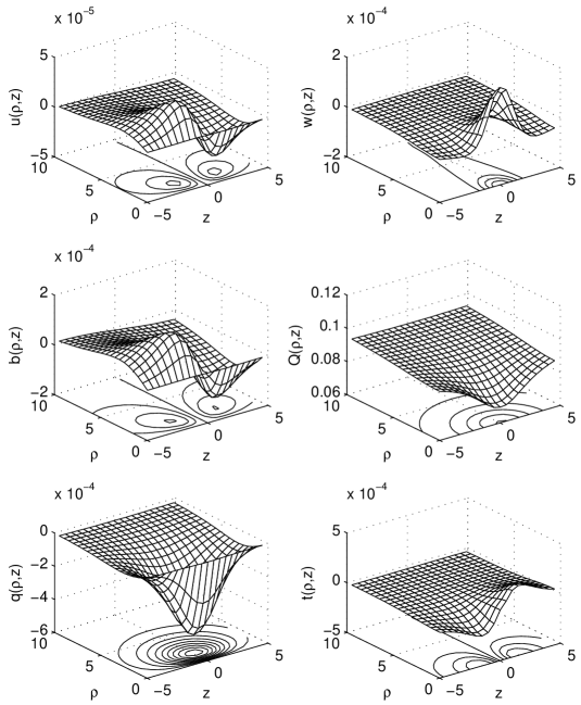
Figure 2: Numerical solution for $(A_{0})_{\rm static}$ in the non-BPS SO(5) theory, with $\omega_{0}=0.1\,ev$. The coordinates $z$ and $\rho$ are given in units of $1/ev$ and the component fields $u$, $w$, $b$, $Q$, $q$, and $t$, defined in Eq. (13), in units of $v$.

In contrast with the BPS case, we see that all of the coefficient functions are nonzero, although $Q$ remains dominant, and that all of these functions, including $Q$, have only axial symmetry, with separate dependence on $\rho$ and $z$.

IV Evolving the chromodyon

In the previous two sections we obtained a static monopole solution and then determined the $A_{0}$ that is required by Gauss’s law when this solution rotates uniformly in SU(2) space. We now take this configuration as the initial condition and let the system evolve as dictated by the equations of motion. We work in the gauge where the uniform rotation has been gauged away, so that the initial configuration $\{(A_{0})_{\rm static},(A_{i})_{\rm static},(\Phi)_{\rm static}\}$ would be a static solution if the MSA were exact. In this gauge, any time dependence arises from corrections to the MSA.

To proceed, we need to specify $\omega_{0}$. It cannot be too big (e.g., so large that the energy arising from the gauge rotation is comparable to the monopole mass) if the original configuration is to be even an approximate solution. A more stringent condition is suggested by the existence of the embedded pure SU(2) monopole described at the end of Sec. II. In order to make sure that our configuration does not evolve toward this other monopole solution, we want the energy associated with the gauge rotation to be less than the mass difference between the two types of static monopoles. On the other hand, taking $\omega_{0}$ to be too small will impose increased computational burdens, because we will have to simulate the evolution for a much longer time in order to see any effect.

We choose $\omega_{0}=0.04\,ev$. The gauge rotation energy corresponding to this is of order $(\omega_{0}/ev)^{2}M_{\rm BPS}\approx 10^{-3}M_{\rm BPS}$, smaller than the mass difference between the two monopole solutions. Because the $A_{0}$ obtained in the previous section is linearly proportional to $\omega_{0}$, the initial data can be obtained by a simple rescaling of the solution shown in Fig. 2.

The Euler-Lagrange equations consist of the evolution equations

$$D_{0}F^{0i}+D_{j}F^{ji}=ie[\Phi,D^{i}\Phi]\,,$$ (1)

$$D_{0}D^{0}\Phi+D_{j}D^{j}\Phi={\partial V(\Phi)\over\partial\Phi}\,,$$ (2)

and the Gauss’s law constraint

$$D_{j}F^{j0}=ie[\Phi,D^{0}\Phi]\,.$$ (3)

We will use the so-called free evolution scheme to simulate this constrained system. In this scheme, we numerically solve the evolution equations, and use the constraints to monitor the accuracy of the evolution. It is well known that direct numerical implementation can have problems with numerical instability. To avoid this, we choose to use the technique in Ref. Abrahams:1995nj to first rewrite the evolution equations in hyperbolic form. To do this, we take a covariant time derivative of Eq. (1) and subtract a covariant spatial derivative of the Gauss’s law constraint, obtaining

$$D^{0}D_{0}F^{0i}+D^{0}D_{j}F^{ji}-D^{i}D_{j}F^{j0}=ie\,D^{0}[\Phi,D^{i}\Phi]-ie\,D^{i}[\Phi,D^{0}\Phi]\,.$$ (4)

Switching the two covariant derivatives on the left-hand side gives

$$D^{0}D_{0}F^{0i}+D_{j}D_{0}F^{ij}+D_{j}D_{i}F_{j0}+2ie[F_{ij},F_{j0}]=ie\,D^{0}[\Phi,D^{i}\Phi]-ie\,D^{i}[\Phi,D^{0}\Phi]\,.$$ (5)

Next, we take a covariant spatial derivative of the Bianchi identity,

$$D_{0}F_{ij}+D_{i}F_{j0}+D_{j}F_{0i}=0\,,$$ (6)

to give

$$D_{j}D_{0}F_{ij}+D_{j}D_{i}F_{j0}=D_{j}D_{j}F_{i0}\,.$$ (7)

We substitute this into Eq. (5) and obtain

$$D^{0}D_{0}F_{i0}+D^{j}D_{j}F_{i0}+2ie[F_{ij},F_{j0}]=ie\,D^{0}[\Phi,D^{i}\Phi]-ie\,D^{i}[\Phi,D^{0}\Phi]\,.$$ (8)

The full set of equations now consists of the definition of $F_{\mu\nu}$ and two wave equations, Eqs. (2) and (8). Equation (1) becomes a second constraint.

One advantage of this hyperbolic formulation is that it does not depend on the gauge condition. Therefore, by assuming an appropriate time-dependent gauge transformation, we can choose $A_{0}$ to be anything we want. In particular, we will set

$$A_{0}({\bf r},t>0)=(A_{0}({\bf r}))_{\rm static}\,,$$ (9)

where $(A_{0})_{\rm static}$ is the solution shown in Fig. 2. The chromodyon configuration constructed previously is an approximate stationary solution with this choice of $A_{0}$. If it were exact, Eq. (9) would correspond to choosing a gauge in which the SU(2) rotation was gauged away. Any time dependence that we observe will correspond to corrections to this approximation.

Once $A_{0}$ has been fixed in this manner, the time-dependent variables in this formulation are $A_{i}$, $\Phi$, and $E_{i}\equiv F_{i0}$. Their initial values at $t=0$ are chosen to be $(A_{i})_{\rm static}$, $(\Phi)_{\rm static}$, and $D_{i}(A_{0})_{\rm static}$. The time derivatives of $A_{i}$ and $\Phi$ at $t=0$ are set equal to zero, while $\partial_{0}E_{i}(t=0)$ is obtained from the constraint Eq. (1). Note that $E_{i}(t=0)$ is $O(\omega_{0})$ and $\partial_{0}E_{i}(t=0)$ is $O(\omega_{0}^{2})$.

                 

                                  (a)                                                         (b)

Figure 3: (a) Using three slabs in the three-dimensional Cartesian coordinates. (b) Axial symmetry is used to update grid points on the off-center slabs.

The system has axial symmetry at $t=0$ and this symmetry will be preserved by the evolution. Usually, a two-dimension grid structure in the $\rho$-$z$ plane is used to discretize an axially symmetric system. However, using cylindrical coordinates to simulate time-dependent systems can easily cause numerical instabilities Pogosian:1999zi . In our implementation, we use the method proposed in Ref. Alcubierre:1999ab . The idea is to discretize the system using three slabs in the three-dimension Cartesian coordinates, as shown in Fig. 3a. Each slab is a two-dimensional grid structure with step size $h$. The central slab lies in the $x$-$z$ plane. The other two slabs are obtained by shifting the central one by $+h$ and $-h$ along the $y$ axis, respectively. At each grid point, any so(5)-valued element is represented by ten real numbers. For each time step, the two wave equations are solved first on the central slab using the finite difference method. Then the axial symmetry is used to update the grid points on the other two slabs. To be precise, we plot the grid structure in Fig. 3b. The axial symmetry tells us that the system will be invariant if we rotate it through the same angle both in real spatial space and in isospin space. For the $\Phi$ field, this means that

$$\Phi({\bf r}_{D},t)=e^{-ih_{3}\theta}e^{-ik_{3}\theta}\Phi({\bf r}_{E},t)e^{ik_{3}\theta}e^{ih_{3}\theta}\,,$$ (10)

where $\theta$ is the angle between ${\bf r}_{E}$ and ${\bf r}_{D}$. For the $A_{i}$ field, it means that

$$A_{i}({\bf r}_{D},t)=e^{-ih_{3}\theta}e^{-ik_{3}\theta}R_{ij}(\theta)A_{j}({\bf r}_{E},t)e^{ik_{3}\theta}e^{ih_{3}\theta}\,,$$ (11)

with $R_{ij}(\theta)$ being the matrix corresponding to a spatial rotation by angle $\theta$ about the $z$-axis. Interpolation is used to calculate $\Phi({\bf r}_{E},t)$ and $A_{i}({\bf r}_{E},t)$ from the values at the neighboring grid points, $A$, $B$, and $C$.

In our simulation, the grid with three slabs covers a space of size 60 (in units of $1/ev$). The open boundary condition is used because of its simplicity. The radius of the monopole is roughly 1 and we focus on studying a region with a radius of 10. This implies that we can only simulate our system up to $t=50$.

Because the system is approximately stationary at $t=0$, the time-dependent parts are very small. In the hyperbolic formulation, we have four fields, $A_{0}$, $A_{i}$, $E_{i}\equiv F_{i0}$, and $\Phi$. Since we have already prescribed $A_{0}$ to be time-independent by Eq. (9), only $A_{i}$, $E_{i}$, and $\Phi$ have time-dependent parts. In our implementation, we separate out the time-dependent parts via

$$A_{i}({\bf r},t)={\bar{A}_{i}}({\bf r})+{\tilde{A}_{i}}({\bf r},t)\,,$$

$$E_{i}({\bf r},t)={\bar{E}_{i}}({\bf r})+{\tilde{E}_{i}}({\bf r},t)\,,$$

$$\Phi({\bf r},t)={\bar{\Phi}}({\bf r})+{\tilde{\Phi}}({\bf r},t)\,,$$ (12)

where ${\tilde{A}_{i}}({\bf r},t=0)={\tilde{E}_{i}}({\bf r},t=0)={\tilde{\Phi}}({\bf r},t=0)=0$. During the evolution, we check how well these time-dependent parts satisfy the Gauss’s law constraint. Theoretically, this constraint should be satisfied at $t=0$ because of the way we construct the initial gauge-rotating system, and should remain satisfied for all $t$. Numerically, however, it is only satisfied up to some finite accuracy. To check how well the Gauss’s law constraint is satisfied, we write the right-hand side of the constraint as a sum of nine terms, and then treat each of these terms as a vector in a ten-dimensional space. We then define the sum of all these vectors (which theoretically should vanish) to be the defect. This defect should remain small as long as our numerical scheme is stable. If the scheme is not stable, the defect will grow exponentially. We calculate the ratio between the maximum norm of the defect and the maximum norm among all of its component vectors. (For both norms we take the maximum over the entire computational domain.) We use this ratio to measure the accuracy to which the Gauss’s law constraint is satisfied. At $t=0$ this ratio is $0.5\times 10^{-2}$, while during the evolution the ratio for the time-dependent parts never exceeds $3\times 10^{-2}$. More details about this can be found in Appendix B.

V Global gauge rotation slow-down

Our initial configuration satisfies the equations of motion to first order in $\omega_{0}$. If this first-order approximation were exact, the solution would be time-independent, so the time-dependent parts in Eq. (12) tell us how the real evolution deviates from this first-order approximation. By analyzing the result of our simulation, we find that we can best fit this deviation in terms of a global gauge rotation. Recall that our initial configuration corresponds to a monopole rotating in SU(2) space about the $k_{3}$ axis with an angular velocity $\omega_{0}$. We made it static by going to a gauge with $A_{0}(\infty)=(\omega_{0}/e)k_{3}$, effectively transforming to a rotating frame. By fixing $A_{0}({\bf r},t)$ as in Eq. (9) we stay within that rotating frame during the evolution. Any slowing of the gauge rotation would appear in this frame as a rotation about the $k_{3}$ axis, but in the opposite direction. Thus, it would correspond to a global gauge rotation generated by

$$\Lambda_{s}(\theta)=e^{-ik_{3}\theta(t)}$$ (1)

with positive $\theta(t)$. The effect would be as if the initial angular velocity $\omega_{0}$ were replaced by

$$\omega_{\rm eff}=\omega_{0}-{d\theta\over dt}\,,$$ (2)

leading to a configuration with smaller color charge and a smaller energy.

The fields $A_{i}$ and $\Phi$ can be expanded in SO(5) components, as in Eq. (4). The first-sector components are unchanged by the rotation generated by $\Lambda_{s}(\theta)$. The second-sector components transform as

$$\left(\begin{array}[]{c}\hat{P}_{(2)}^{1}\\ \hat{P}_{(2)}^{2}\\ \hat{P}_{(2)}^{3}\end{array}\right)=\left(\begin{array}[]{ccc}\cos\theta&-\sin\theta&0\\ \sin\theta&\cos\theta&0\\ 0&0&1\end{array}\right)\left(\begin{array}[]{c}P_{(2)}^{1}\\ P_{(2)}^{2}\\ P_{(2)}^{3}\end{array}\right)$$ (3)

while the third-sector components decompose into two doublets transforming according to

$$\left(\begin{array}[]{c}\hat{P}_{(3)}^{1}\\ \hat{P}_{(3)}^{2}\\ \hat{P}_{(3)}^{3}\\ \hat{P}_{(3)}^{4}\end{array}\right)=\left(\begin{array}[]{cccc}\cos(\theta/2)&-\sin(\theta/2)&0&0\\ \sin(\theta/2)&\cos(\theta/2)&0&0\\ 0&0&\cos(\theta/2)&-\sin(\theta/2)\\ 0&0&\sin(\theta/2)&\cos(\theta/2)\end{array}\right)\left(\begin{array}[]{c}P_{(3)}^{1}\\ P_{(3)}^{2}\\ P_{(3)}^{3}\\ P_{(3)}^{4}\end{array}\right)\,.$$ (4)

Let us define

$$\Delta\Phi({\bf r},t;\theta) = \left[\frac{}{}\Lambda_{s}(\theta){\bar{\Phi}}({\bf r})\Lambda_{s}^{-1}(\theta)-{\bar{\Phi}}({\bf r})\frac{}{}\right]-{\tilde{\Phi}}({\bf r},t)\,,$$

$$\Delta A_{i}({\bf r},t;\theta) = \left[\frac{}{}\Lambda_{s}(\theta){\bar{A}_{i}}({\bf r})\Lambda_{s}^{-1}(\theta)-{\bar{A}_{i}}({\bf r})\frac{}{}\right]-{\tilde{A}_{i}}({\bf r},t)\,,$$ (5)

where ${\tilde{\Phi}}({\bf r},t)$ and ${\tilde{A}_{i}}({\bf r},t)$ are from our numerical simulation. If the time evolution of our configuration were completely due to a slowing of the global gauge rotation, then for any given time $t$ there would be a single $\theta(t)$ that would make ${\Delta\Phi}({\bf r},t;\theta)$ and ${\Delta A_{i}}({\bf r},t;\theta)$ both vanish for all values of $\bf r$. To see how close we are to this situation, we can extract a value for $\theta$ by several different methods and then compare these values. First, we obtain $\theta$ from the second-sector components of $\Phi$ by minimizing

$${\rm Tr\,}\left[\Delta\Phi_{(2)}({\bf r},t;\theta)\right]^{2}$$ (6)

at various points. In Fig. 4a we show the $\theta$ obtained in this manner for a series of points along the $x$-axis. As can be seen, the $\theta$’s thus obtained are only weakly position-dependent. We can also define a spatially averaged $\theta$ by finding the value that minimizes quantities such as

$${\cal N}(t,\theta)=\int\!\!\!\int\!\!\!\int_{r\leq R_{e}}\left\{\leavevmode\hbox{Tr}\left[\Delta A_{i}({\bf r},t;\theta)\right]^{2}+\leavevmode\hbox{Tr}\left[\Delta\Phi({\bf r},t;\theta)\right]^{2}\right\}dxdydz\,,$$ (7)

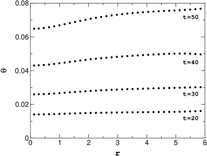
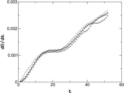
                                          (a)                                                                     (b)        

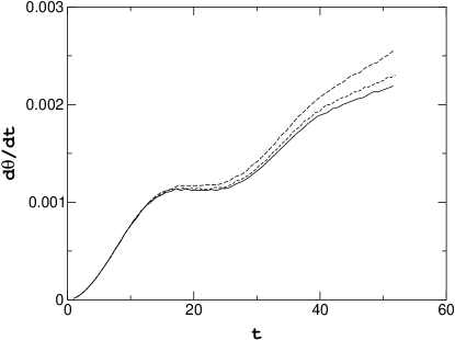
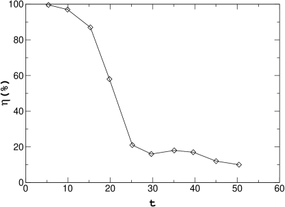
                                  (c)                                                                     (d)

Figure 4: (a) Fitted values of $\theta$ at grid points along the positive $x$-axis. (b) Values of $d\theta/dt$ obtained by fitting with various sets of component fields. Circles indicate fits using $\Phi$, squares fits using $A_{i}$, the solid line fits using $A_{i(3)}$, and the dashed line fits using $A_{i(2)}$. (c) Comparison of results using different grid sizes. The long dashed curve, the dashed curve, and the solid line curve are calculated using $\Delta h=0.18(ev)^{-1}$, $\Delta h=0.12(ev)^{-1}$, and $\Delta h=0.08(ev)^{-1}$ grid sizes, respectively. (d) Plot of $\eta(t)$, defined by Eq. (8), which indicates the fraction of the time dependence that cannot be accounted for by the global gauge rotation. In all four figures distances and times are given in units of $1/ev$ and $\omega_{0}=0.04ev$.

where $R_{e}$ is the size of the physical region of interest. In Fig. 4b, we compare the results for $d\theta/dt$ that are obtained by restricting ${\cal N}$ in several different ways: using only $\Phi$ or only $A_{i}$, or using just the second-sector or just the third-sector components of $A_{i}$. [The first-sector components are invariant under $\Lambda_{s}(\theta)$, and so cannot affect the fitting of $\theta$.] We see that all of these methods give essentially the same results, again consistent with the interpretation in terms of a spatially uniform global gauge rotation. In order to indicate the convergence of our simulations, in Fig. 4c we show three curves for $\omega_{0}=0.04ev$, using successively finer grid structures.

We can also ask how much of the time-dependence can be accounted for by this uniform rotation. To this end, we divide the residual norm after fitting $\theta$ by the norm of all the component fields in the time-dependent parts, and define

$$\eta(t)=\frac{{\cal N}(t,\theta(t))}{{\cal N}(t,0)}\,.$$ (8)

We plot $\eta$ for our simulation in Fig. 4d. We see that, although initially the global gauge rotation accounts for only a small part of the time dependence, at large times it is clearly the dominant component.

We see from the data in Fig. 4 that $d\theta/dt$ increases with time (although not uniformly), with a corresponding decrease in $\omega_{\rm eff}$. This can be interpreted as the sum of two effects, as shown in Fig. 5. One is an overall oscillation pattern that appears to be a transient effect caused by the relaxation of the system after the initial excitation. The other effect is a linearly increasing $d\theta/dt$. By the end of our simulation, at $t=52(ev)^{-1}$, about 5% of the initial angular velocity has been lost. We do not see any indication that this slowing down process will stop, and expect that $\omega_{\rm eff}$ would eventually tend to zero if the simulation could be carried out for long enough.

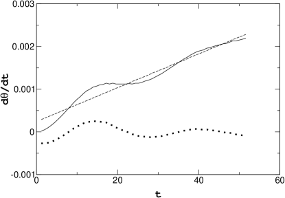
Figure 5: Decomposition of $d\theta/dt$ (solid line) into linear and oscillating components. Time is in units of $1/ev$, and $\omega_{0}=0.04ev$.

The energy that the chromodyon loses through the slowing of the gauge rotation must be carried away by radiation of the massless gauge fields in the unbroken non-Abelian subgroup. (Indeed, much of the nonrotational contribution to $\eta$ at early times can presumably be attributed to the creation of the radiation field.) It is of interest to know how this radiation depends on $\omega_{0}$. We can use the slope of the constant part in Fig. 5 to approximate $d^{2}\theta/dt^{2}$ for $\omega_{0}=0.04ev$. In Table 1 we show the results for this as well as the corresponding results for simulations with two other values of $\omega_{0}$. Recalling from Eq. (7) that the energy associated with the phase rotation is proportional to $\omega^{2}$, we see that this data is consistent with

$${dE_{\rm ch}\over dt}\sim\omega_{\rm eff}{d\omega_{\rm eff}\over dt}\sim\omega_{\rm eff}^{4}\,.$$ (9)

$\omega_{0}$	$d^{2}\theta/dt^{2}$	$(ev/\omega_{0}^{3})\,d^{2}\theta/dt^{2}$
$0.01\,ev$	$8.0\times 10^{-7}\,(ev)^{2}$	0.80
$0.02\,ev$	$6.2\times 10^{-6}\,(ev)^{2}$	0.78
$0.04\,ev$	$4.6\times 10^{-5}\,(ev)^{2}$	0.72

Table 1: Dependence of the deceleration of the initial global gauge rotation on the initial angular velocity $\omega_{0}$.

We can understand this dependence by considering the energy flux carried by the radiation of the massless non-Abelian gauge fields in the unbroken subgroup. This should be given by the analogue of the electromagnetic Poynting vector,

$$T_{i}\,\sim\,\epsilon_{ijk}\leavevmode\hbox{Tr}\,\hat{E}_{j}\hat{B}_{k}\,,$$ (10)

where the hats indicate the $O(1/r)$ radiation components of the field strengths. Because the initial chromodyon configurations that we constructed satisfied the static field equations to first order in $\omega_{0}$, these radiation fields must be each at least second order in $\omega_{0}$, so that $T_{i}\sim\omega^{4}_{0}$.

VI Concluding remarks

Magnetic monopoles can be promoted to dyons by time-dependent excitation of their U(1) global gauge zero modes. In this paper we have addressed the question of whether monopoles in theories with non-Abelian unbroken symmetries can be promoted to chromodyons — monopoles with non-Abelian electric charge — by a similar excitation of their non-Abelian global gauge zero modes. It has long been known that the answer is negative if the magnetic charge has a non-Abelian component, because there are then topological obstructions that preclude the existence of a chromodyon. However, there are also monopoles with purely Abelian asymptotic magnetic charge, for which there is no such obstruction, that could potentially have chromodyonic counterparts. We have examined one such case here, using a constructive approach. We started with a configuration with a globally rotating non-Abelian phase, and thus a nonzero chromo-electric charge, and then numerically evolved it to see whether it would settle down in a stable static solution. In our simulations we found instead that the effective rate of gauge rotation slows down, so that the chromodyon continually loses energy and chromo-electric charge. Although we were not able to continue the simulation until this charge was completely lost, every indication suggests that this would be the final state of the system.

It is instructive to compare our results with those that would have been obtained by applying our methods in the theory with SU(2) broken to U(1), where we know that there is a dyon with Abelian electric charge. Because there is no analogue of the cloud radius zero mode, with its associated complications, we can work in the BPS limit, where analytic expressions are available.

Our approach would start with the static monopole solution

$$A_{i}^{a} = \epsilon_{aim}{\hat{r}_{m}}A(r)\,,$$ (1)

$$\Phi^{a} = {\hat{r}_{a}}\,H(r)\,,$$ (3)

with

$$A(r) = {v\over\sinh evr}-{1\over er}\,,$$ (4)

$$H(r) = v\coth evr-{1\over er}\,.$$ (5)

Applying a global U(1) phase rotation and then gauge transforming back to a static gauge would yield

$$(A_{0}^{a})_{\rm static}={\hat{r}_{a}}Q(r)\,,$$ (6)

where

$$Q(r)={\omega_{0}\over ev}\left[v\coth evr-{1\over er}\right]\,.$$ (7)

From the $1/r$ term in this expression, we see that the asymptotic electric field is

$$E_{i}^{a}=\hat{r}_{a}\hat{r}_{i}\,{q_{E}\over r^{2}}\,,$$ (8)

where

$$q_{E}={1\over e}\left({\omega_{0}\over ev}\right)\,.$$ (9)

The energy of this configuration is

$$E={4\pi v\over e}\left[1+{e^{2}q_{E}^{2}\over 2}\right]\,,$$ (10)

where the first term represents the mass of the original monopole and the second is the additional energy due to the phase rotation.

As in the chromodyon case, this initial configuration is only an approximate solution of the equations of motion. The exact dyon solution with charge $q_{E}$ is given by Prasad:1975kr ; Bogomolny:1975de

$$A(r) = {v^{\prime}\over\sinh ev^{\prime}r}-{1\over er}\,,$$ (11)

$$H(r) = \cosh\gamma\left[v^{\prime}\coth ev^{\prime}r-{1\over er}\right]\,,$$ (13)

$$Q(r) = \sinh\gamma\left[v^{\prime}\coth ev^{\prime}r-{1\over er}\right]\,,$$ (15)

where $\gamma$ is determined by the ratio of electric and magnetic charges and is given by

$$\sinh\gamma=eq_{E}$$ (16)

and $v^{\prime}=v/\cosh\gamma$. It has an energy

$$E={4\pi v\over e}\sqrt{1+(eq_{E})^{2}}$$ (17)

and corresponds to phase rotating with an angular velocity

$$\omega=ev^{\prime}\sinh\gamma={e^{2}vq_{E}\over\sqrt{1+(eq_{E})^{2}}}\,.$$ (18)

Thus, our construction would start with a configuration that has a core radius that is a factor $\sqrt{1+(eq_{E})^{2}}$ smaller than that of the exact solution, and an angular velocity that is larger by the same factor. (The smaller core radius produces an decrease in the phase rotation moment of inertia that exactly compensates for the increase in angular velocity, thus yielding the same electric charge.) The energy of this initial configuration exceeds that of the exact dyon solution by an amount of order $q_{E}^{4}$.

It is easy to see what will happen if the initial configuration of Eqs. (5) and (7) is allowed to evolve. Because radiation of the massive charged gauge field is energetically suppressed, the electric charge of the dyonic configuration will be conserved. Hence, as the initial system relaxes it will tend toward the static dyon solution of the same charge. It will shed energy by radiating massless photons, but the amount of this energy loss is constrained by the fact that exact dyon mass places a lower bound on the energy. As the dyon radiates its phase rotation will slow down and its core will expand. For small electric charge (i.e., $eq_{E}\ll 1$), this slowing and expansion will both be small, and the system will quickly approach its final state. In particular, the slowing of the phase rotation will be far less than that which we found in our non-Abelian simulation.

Thus, our numerical simulations provide strong evidence against the existence of static chromodyons in a theory with SO(5) broken to SU(2)$\times$U(1). Because it is hard to see how enlarging the unbroken symmetry to a different non-Abelian group would stabilize the chromodyon, we expect that similar results would hold for other choices of gauge group and symmetry breaking. Of course, numerical simulations cannot provide a rigorous proof. Even apart from issues related to numerical accuracy, there is always the possibility that the specific choice of initial configuration played a crucial role. For example, it is logically conceivable (although we think it quite implausible) that there is some special choice or range of $\omega_{0}$ that would have led to a stable chromodyon. Another possibility is that there are chromodyon solutions, but that these exist only for some minimum value of the chromo-electric charge. In this case, the solutions would not be continuously related to the purely magnetic monopole, and so might not be found by our method. Although we cannot exclude this possibility, it seems to us to be rather unlikely. Hence, subject to these caveats, we conclude that static chromodyon solutions do not exist.

Appendix A Gauss’s law equation with axial symmetry

As discussed in Sec. III, when we gauge rotate the spherically symmetric static non-BPS monopole solution, the resulting Gauss’s law equation has only axial symmetry and consists of six coupled partial differential equations for the six coefficient functions $u$, $w$, $b$, $Q$, $q$, and $t$ appearing in the $A_{0}$ ansatz of Eq. (13). We write out the detailed forms of these equations below. Here, $A$, $H$, $G$, $K$, $F$, and $J$ are the functions, defined by Eq. (7), that specify the static non-BPS monopole solution and that are shown in Fig. 1. To simplify the equations, we have set $e=1$ throughout; the explicit factors of $e$ can be recovered by simple dimensional analysis.

The two equations corresponding to first-sector components are

$$\partial_{\rho\rho}u+{1\over\rho}\partial_{\rho}u-{u\over\rho^{2}}+\partial_{zz}u-2{\rho\over r}A\partial_{z}w+2{z\over r}A\partial_{\rho}w-4F\partial_{z}q+4F\partial_{\rho}t$$

$$+2{\rho\over r}(\partial_{r}F)t-2{z\over r}(\partial_{r}F)q-6{\rho\over r}AFt+2{\rho\over r}FGt-{\rho\over r}KJt+{\rho\over r}HJt$$

$$+2{z\over r}AFq-2{z\over r}FGq+{z\over r}KJq+3{z\over r}HJq-2{\rho^{2}\over r^{2}}A^{2}u-{z\rho\over r^{2}}A^{2}w+{z\rho\over r^{2}}H^{2}w$$

$$-{z^{2}\over r^{2}}A^{2}u-{z^{2}\over r^{2}}H^{2}u-F^{2}b+J^{2}b-3F^{2}u-J^{2}u-2{1\over r}Au=0\,,$$ (1)

$$\partial_{\rho\rho}w+{1\over\rho}\partial_{\rho}w+\partial_{zz}w+4F\partial_{z}t+4F\partial_{\rho}q+2{\rho\over r}A\partial_{z}u-2{z\over r}A\partial_{\rho}u+2{z\over r}(\partial_{r}F)t$$

$$+2{\rho\over r}(\partial_{r}F)q+4{1\over\rho}Fq-2{z\over\rho}{1\over r}Au-{\rho^{2}\over r^{2}}A^{2}w-{\rho^{2}\over r^{2}}H^{2}w-2{z^{2}\over r^{2}}A^{2}w$$

$$-2{\rho\over r}AFq+2{\rho\over r}FGq-{\rho\over r}KJq-3{\rho\over r}HJq-6{z\over r}AFt+2{z\over r}FGt$$

$$-{z\over r}KJt+{z\over r}HJt-{\rho z\over r^{2}}A^{2}u+{\rho z\over r^{2}}H^{2}u-F^{2}Q+J^{2}Q-3F^{2}w-J^{2}w=0\,.$$ (2)

The two second-sector equations can be obtained from these simply by making the substitutions

$$u\rightarrow b\,, w\rightarrow Q\,,$$

$$A\rightarrow G\,, H\rightarrow K\,.$$ (3)

Finally, the third-sector equations are

$$\partial_{\rho\rho}q+{1\over\rho}\partial_{\rho}q-{q\over\rho^{2}}+\partial_{zz}q+{\rho\over r}A\partial_{z}t-{\rho\over r}G\partial_{z}t+F\partial_{z}b+F\partial_{z}u-{z\over r}A\partial_{\rho}t+{z\over r}G\partial_{\rho}t$$

$$-F\partial_{\rho}Q-F\partial_{\rho}w-2{\rho\over r}(\partial_{r}F)Q-{1\over 2}{\rho\over r}(\partial_{r}F)w+{1\over 2}{z\over r}(\partial_{r}F)b+{1\over 2}{z\over r}(\partial_{r}F)u$$

$$+{\rho\over r}\left[{1\over 2}AFQ-{1\over 2}FGQ+{1\over 4}HJQ+{3\over 4}JKQ-{1\over 2}AFw+{1\over 2}FGw-{3\over 4}HJw-{1\over 4}JKw\right]$$

$$+{z\over r}\left[-{1\over 2}AFb+{1\over 2}FGb-{1\over 4}HJb-{3\over 4}JKb+{1\over 2}AFu-{1\over 2}FGu+{3\over 4}HJu+{1\over 4}JKu\right]$$

$$-{1\over 2}A^{2}q-{1\over 2}G^{2}q-{1\over 4}H^{2}q-{1\over 2}HKq-{1\over 4}K^{2}q-4F^{2}q-2J^{2}q-{1\over r}Aq-{1\over r}Gq=0\,,$$ (4)

$$\partial_{\rho\rho}t+{1\over\rho}\partial_{\rho}t+\partial_{zz}t+F\partial_{z}Q-F\partial_{z}w+F\partial_{\rho}b-F\partial_{\rho}u-{\rho\over r}A\partial_{z}q+{\rho\over r}G\partial_{z}q+{z\over r}A\partial_{\rho}q$$

$$-{z\over r}G\partial_{\rho}q+{1\over 2}{z\over r}(\partial_{r}F)Q-{1\over 2}{z\over r}(\partial_{r}F)w+{1\over 2}{\rho\over r}(\partial_{r}F)b-{1\over 2}{\rho\over r}(\partial_{r}F)u$$

$$+{1\over\rho}Fb-{1\over\rho}Fu+{z\over\rho}{1\over r}Aq-{z\over\rho}{1\over r}Gq$$

$$+{\rho\over r}\left[-{1\over 2}AFb+{3\over 2}FGb-{1\over 4}HJb+{1\over 4}JKb-{3\over 2}AFu+{1\over 2}FGu+{1\over 4}HJu-{1\over 4}JKu\right]$$

$$+{z\over r}\left[-{1\over 2}AFQ+{3\over 2}FGQ-{1\over 4}HJQ+{1\over 4}JKQ-{3\over 2}AFw+{1\over 2}FGw+{1\over 4}HJw-{1\over 4}JKw\right]$$

$$-6F^{2}t-{1\over 2}A^{2}t+AGt-{1\over 2}G^{2}t-{1\over 4}H^{2}t+{1\over 2}HKt-{1\over 4}K^{2}t=0\,.$$ (5)

Appendix B Monitoring the Gauss’s law constraint

Analytically, the Gauss’s law constraint should remain satisfied throughout the evolution if it is satisfied by the initial data. In our numerical calculation, we keep monitoring how well the constraint is satisfied and use this as a way to check the accuracy of our numerical methods.

The Gauss’s law constraint is

$$D_{j}F^{j0}=ie[\Phi,D^{0}\Phi]\,.$$ (1)

We can use Eq. (12) to expand this into time-dependent and time-independent parts. Focusing on the time-dependent part, we have the requirement that

$$0 = \partial_{j}{\tilde{E}_{j}}+ie[{\tilde{A}_{j}},{\bar{E}_{j}}]+ie[{\bar{A}_{j}},{\tilde{E}_{j}}]+ie[{\tilde{A}_{j}},{\tilde{E}_{j}}]-\,ie[{\bar{\Phi}},\partial_{0}{\tilde{\Phi}}]-ie[{\tilde{\Phi}},\partial_{0}{\tilde{\Phi}}]$$ (3)

$$-\,ie^{2}[{\bar{\Phi}},i[A_{0},{\tilde{\Phi}}]]-ie^{2}[{\tilde{\Phi}},i[A_{0},{\bar{\Phi}}]]-ie^{2}[{\tilde{\Phi}},i[A_{0},{\tilde{\Phi}}]]\,.$$

To demonstrate that the Gauss’s law constraint is satisfied in our numerical calculation, we calculate these nine terms using our numerical results and then define their sum to be the defect. Since the defect is an so(5) element, we can define its norm to be the square root of the trace of its square. In Figs. 6 and 7 we plot on the $x$-$z$ plane the norm of the defect and, for comparison, the norm of the first term, both at $t=34.2(ev)^{-1}$. As we can see, the defect is about two orders of magnitude smaller than the first term, indicating that the Gauss’s law constraint is satisfied very well. We define the defect level to be the ratio of the maximum norm of the defect and the maximum norm among all terms. (Both maxima are found over the entire computation domain.) For example, at $t=34.2(ev)^{-1}$, the maximum norm of the defect is about $8\times 10^{-6}$, while the maximum norm of the first term (which is larger than that of any of the other terms) is about $4\times 10^{-4}$. This give a defect level of about $0.02$.

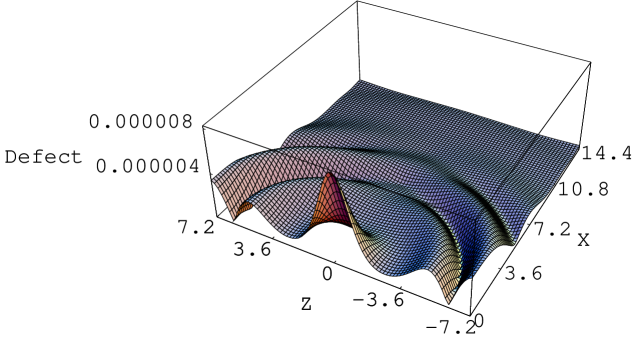
Figure 6: The norm of the defect of the Gauss’s law constraint at $t=34.2(ev)^{-1}$. Since the system has an axial symmetry along the $z$ axis, we plot the results on the $x$-$z$ plane. Distances are given in units of $1/ev$, and the defect is in units of $v$.

Figure 7: The norm of the first term in Eq. (3) at $t=34.2(ev)^{-1}$. Since the system has an axial symmetry along the $z$ axis, we plot the results on the $x$-$z$ plane. Distances are given in units of $1/ev$, and the defect is in units of $v$.

References

- (1) A. Abouelsaood, Nucl. Phys. B 226, 309 (1983).
- (2) P. C. Nelson and A. Manohar, Phys. Rev. Lett. 50, 943 (1983).
- (3) A. P. Balachandran, G. Marmo, N. Mukunda, J. S. Nilsson, E. C. G. Sudarshan and F. Zaccaria, Phys. Rev. Lett. 50, 1553 (1983).
- (4) A. P. Balachandran, G. Marmo, N. Mukunda, J. S. Nilsson, E. C. G. Sudarshan and F. Zaccaria, Phys. Rev. D 29, 2919 (1984).
- (5) A. P. Balachandran, G. Marmo, N. Mukunda, J. S. Nilsson, E. C. G. Sudarshan and F. Zaccaria, Phys. Rev. D 29, 2936 (1984).
- (6) P. A. Horvathy and J. H. Rawnsley, J. Math. Phys. 27, 982 (1986).
- (7) P. A. Horvathy and J. H. Rawnsley, Phys. Rev. D 32, 968 (1985).
- (8) E. J. Weinberg, Phys. Lett. B 119, 151 (1982).
- (9) B. Julia and A. Zee, Phys. Rev. D 11, 2227 (1975).
- (10) G. ’t Hooft, Nucl. Phys. B 79, 276 (1974).
- (11) A. M. Polyakov, JETP Lett. 20, 194 (1974) [Pisma Zh. Eksp. Teor. Fiz. 20, 430 (1974)].
- (12) P. C. Nelson, Phys. Rev. Lett. 50, 939 (1983).
- (13) P. C. Nelson and S. Coleman, Nucl. Phys. B 237, 1 (1984).
- (14) W. Auzinger, G. Kneisl, O. Koch, and E. B. Weinmuller, Numerical Algorithms 33, 27 (2003).
- (15) K. Lee, E. J. Weinberg and P. Yi, Phys. Rev. D 54, 6351 (1996)
- (16) X. Chen, H. Guo and E. J. Weinberg, Phys. Rev. D 64, 125004 (2001)
- (17) A. Abrahams, A. Anderson, Y. Choquet-Bruhat and J. W. . York, Phys. Rev. Lett. 75, 3377 (1995)
- (18) L. Pogosian and T. Vachaspati, Phys. Rev. D 62, 105005 (2000)
- (19) M. Alcubierre, S. Brandt, B. Brugmann, D. Holz, E. Seidel, R. Takahashi and J. Thornburg, Int. J. Mod. Phys. D 10, 273 (2001)
- (20) M. K. Prasad and C. M. Sommerfield, Phys. Rev. Lett. 35, 760 (1975).
- (21) E. B. Bogomolny, Sov. J. Nucl. Phys. 24, 449 (1976) [Yad. Fiz. 24, 861 (1976)].