Entanglement and purity of single- and two-photon states

Abstract

Whereas single- and two-photon wave packets are usually treated as pure states, in practice they will be mixed. We study how entanglement created with mixed photon wave packets is degraded. We find in particular that the entanglement of a delocalized single-photon state of the electro-magnetic field is determined simply by its purity. We also discuss entanglement for two-photon mixed states, as well as the influence of a vacuum component.

I Introduction

Consider an entangled state containing one or more photons. By how much is the entanglement degraded when the photon wave packets are described by mixed rather than pure states? For example, suppose Alice and Bob are given a two-photon polarization-entangled state Ou and Mandel (1988); Sergienko et al. (1995); Kwiat et al. (1995, 1999); U’Ren et al. (2005)—say the singlet state—but they are not told what the color of the photons is. All they know is the photons are either both blue or both green. Does their ignorance reduce the amount of entanglement they possess? The answer in this case is negative: the entanglement is still one ebit, even though the overall state is mixed. After all, they could, in principle at least, apply a local measurement on each photon that measures its color but not its polarization. That way they are guaranteed to end up with a pure maximally entangled state. The fact that polarization and color are independent degrees of freedom is crucial here.

Suppose now Alice and Bob are given a mode-entangled state Zanardi (2002); van Enk (2003); Shi (2003) containing merely a single delocalized photon Tan et al. (1991); Hardy (1994); Babichev et al. (2004); Björk et al. (2001); Hessmo et al. (2004); van Enk (2005)

$$|\psi\rangle:=\frac{|0\rangle_{A}|1\rangle_{B}+|1\rangle_{A}|0\rangle_{B}}{\sqrt{2}},$$ (1)

where $A$ and $B$ denote specific modes in Alice’s and Bob’s labs and $|0\rangle$ and $|1\rangle$ denote Fock states with zero and one photon, respectively. The notation used implies that modes $A$ and $B$ are well-defined. But suppose that Alice and Bob actually do not know what the color of the single delocalized photon is, green or blue (each with 50% probability). Or suppose they do not know the polarization of the photon, only that it is either left-hand or right-hand circularly polarized. Then they really should ascribe a mixed state to their field modes: an equal mixture of $|\psi\rangle$ and the similar state

$$|\psi^{\prime}\rangle:=\frac{|0\rangle_{A^{\prime}}|1\rangle_{B^{\prime}}+|1\rangle_{A^{\prime}}|0\rangle_{B^{\prime}}}{\sqrt{2}},$$ (2)

where the primed modes refer to modes of different color or different polarization. In Section III we will find the logarithmic negativity Vidal and Werner (2002); Plenio (2005) of this mixed state to be $E_{{\cal N}}=\log_{2}(1+\sqrt{1/2})<1$, so that in this case Alice’s and Bob’s state does lose some of its glamour [a pure state of the form (1) would, obviously, contain one ebit of entanglement]. Note that, indeed, Alice and Bob cannot use the same local filtering measurement of frequency to filter their state to a pure entangled state: as soon as a photon is detected on, say, Bob’s side, the state collapses to either $|0\rangle_{A}|1\rangle_{B}$ or $|0\rangle_{A^{\prime}}|1\rangle_{B^{\prime}}$, and not to the desired pure entangled state $|\psi\rangle$ or $|\psi^{\prime}\rangle$. Alternatively, a nonlocal filtering measurement of color could upgrade Alice’s and Bob’s state to a pure entangled state, but that nonlocal operation could and would increase the amount of entanglement. The distinguishing feature of this example compared to the previous one is that color or polarization and mode are dependent degrees of freedom. More precisely, color and polarization are part of what defines a mode. (Note, by the way, that we can, of course, calculate the logarithmic negativity of the state in the first example as well. The result (see Appendix) is that it indeed equals unity.)

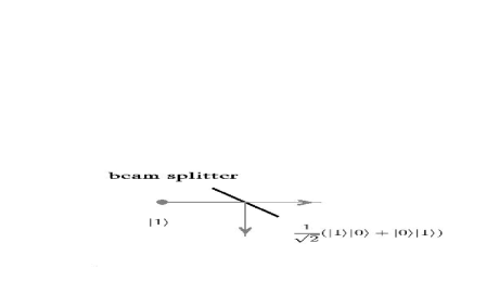
Figure 1: A single photon impinges on a 50/50 beam splitter and one ebit of entanglement is created between the two output ports. How does the entanglement change when the input photon is in a mixed state?
Answer: When we use the logarithmic negativity Vidal and Werner (2002); Plenio (2005) as our entanglement monotone of choice we find $E_{{\cal N}}=\log_{2}(1+\sqrt{{\rm purity}}$), in terms of the purity Tr$\rho^{2}$ of the input state (see Section III).

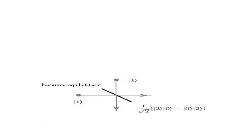
Figure 2: Two identical photons impinge on a 50/50 beam splitter: what is the entanglement at the output?
Answer: 1 ebit, similarly to the answer in Fig.1: the output is a delocalized photon pair.

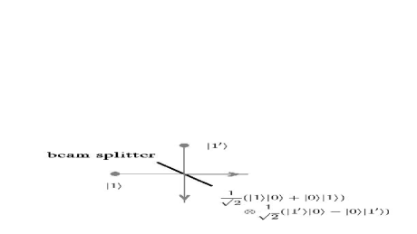
Figure 3: Two distinguishable photons (with, say, orthogonal polarizations or different colors) impinge on a 50/50 beam splitter: what is the entanglement at the output?
Answer: 2 ebits (2 equivalent versions of an entangled delocalized single-photon state) .

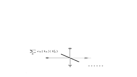
Figure 4: Two distinguishable photons with orthogonal polarizations impinge on a 50/50 beam splitter. When there is already entanglement between the polarization degrees of freedom in the input state, what is the entanglement at the output?
Answer: $E_{\rm out}=2+E_{\rm in}/2$ for the entropy of entanglement, generalizing the answer illustrated in Fig. 3 (see Section IV).
How does this answer change when the input state is mixed?
Answer: it’s complicated …see Section IV for details.

The purpose of this paper is to continue investigating questions of this sort: by how much is the entanglement of single- or two-photon states degraded when the photon wave packets are not pure but mixed? See Figs. 1–4 for typical examples of questions considered in the present paper. The motivation for this research is, of course, the simple fact that typically any photon produced in an experiment is represented by a mixed state Grice and Walmsly (1997); U’Ren et al. (2005); Legero et al. (2006); Raymer et al. (2005). For instance, even if one’s source produces a Fourier-limited wave packet, in practice one will not know exactly the timing of the wave packet, or the exact central frequency, or the exact width. For another example, consider a single photon heralded by detection of the other photon of a down-converted pair of photons. Whenever there is some entanglement between the two photons, tracing out one photon necessarily leaves the remaining photon in a mixed state. Our study complements those in Refs. Humble and Grice (2007, 2008) where the effects of spectral entanglement on polarization degrees of freedom are investigated.

In Section II we start out by collecting some useful results about the description of single- and two-photon wave packets to be used in later sections. In Section III we focus our attention on entangled states that can be generated by splitting a single photon on a 50/50 beam splitter. Ideally that leads to an output state with one ebit of entanglement, but, as we will show, the entanglement resulting from splitting a mixed single-photon input state is less than one ebit but turns out to be a simple function of its purity. In the same Section we will also consider the more realistic case of a nonzero vacuum component of the state of the field and its effect on entanglement. In Section IV we consider typical mixed states of two orthogonally polarized photons arising from type-II down conversion, and in that case too we consider the effects of the presence of a (large) vacuum component. We also compare the mode entanglement one obtains by splitting both photons on a 50/50 beam splitter with the entanglement that may already be present in the input state between two orthogonally polarized modes, and find one may increase the amount of entanglement that way. We conclude the paper with a summary that also discusses some possible extensions of the present work.

II Single- and two-photon wave packets: preliminaries

II.1 Single photons

Consider a single photon of a definite polarization propagating in a well-defined direction. Then a pure state can be described in terms of continuous modes Blow et al. (1990) as

$$|1_{\psi}\rangle=\int dt\widetilde{\psi}(t)a^{\dagger}(t)|{\rm v}\rangle,$$ (3)

where $|{\rm v}\rangle$ is the vacuum state, $a^{\dagger}(t)$ an operator that creates a photon at time $t$ and $\widetilde{\psi}(t)$ the temporal mode function of the wave packet. Often it is more useful to Fourier transform this representation into frequency space, and describe the same state by

$$|1_{\psi}\rangle=\int d\omega\psi(\omega)a^{\dagger}(\omega)|{\rm v}\rangle.$$ (4)

Typically, the function $\psi(\omega)$ will be appreciable only in a small bandwidth $\sigma$ around a central frequency $\omega_{0}$, with $\sigma\ll\omega_{0}$, and the wave packet (4) describes a quasi-monochromatic photon. Since the creation operators bear the relation

$$a^{\dagger}(t)=\frac{1}{\sqrt{2\pi}}\int d\omega a^{\dagger}(\omega)e^{-i\omega t},$$ (5)

the spectral shape $\psi(\omega)$ is thus completely determined by the temporal mode $\widetilde{\psi}(t)$ in the sense that

$$\psi(\omega)=\frac{1}{\sqrt{2\pi}}\int dt\widetilde{\psi}(t)e^{-i\omega t}.$$ (6)

The single-photon states displayed so far are pure. Mixed states of single photons arise, e.g., when they are part of a multipartite system and we trace over the other parties; or if one of the transverse degrees of freedom of the photon is traced out; or if we are simply ignorant about one or more of the properties of the photon. In any case the mixed state of a single photon is described in terms of the density matrix

$$\rho_{1}=\int d\lambda P(\lambda)|1_{\psi_{\lambda}}\rangle\langle 1_{\psi_{\lambda}}|.$$ (7)

Here $\lambda$ stands for any parameter or combination of parameters that can possibly be involved in the mode function, although no concrete form is given yet. Some good examples of what $\lambda$ could stand for are arrival time (”time jitter”), central frequency (”frequency jitter”), the width of the (Fourier-limited) wave packet, etcetera Legero et al. (2006). When writing the mixed state in terms of parameters with such a clear physical meaning, the states $|1_{\psi_{\lambda}}\rangle$’s will in general not be orthogonal. However, we can always diagonalize the density matrix, and rewrite it as a discrete sum involving orthogonal states,

$$\rho_{1}=\sum_{k}p_{k}|1_{k}\rangle\langle 1_{k}|.$$ (8)

Here $p_{k}$ and $|1_{k}\rangle$ are eigensolutions to

$$\rho_{1}|1_{k}\rangle=p_{k}|1_{k}\rangle$$ (9)

with

$$\langle 1_{j}|1_{k}\rangle=\delta_{jk},$$ (10)

and $\sum_{k}p_{k}=1$. For our purpose of calculating entanglement of single-photon states, the latter representation is often more useful.

II.2 Two photons

Now consider states of exactly two photons. Since we have in mind the two-photon component of the state produced by type-II down conversion Hong and Mandel (1985); Ou et al. (1990); Grice and Walmsly (1997), we assume the photons have orthogonal polarizations. We will simply indicate the ordinary and extraordinary polarizations by ”H” and ”V”. Pure and mixed states for such photon pairs can then be expressed as

$$|2_{\psi}\rangle=\int d\omega\int d\omega^{\prime}\psi(\omega,\omega^{\prime})a_{H}^{\dagger}(\omega)a_{V}^{\dagger}(\omega^{\prime})|{\rm v}\rangle,$$ (11)

and

$$\rho_{2}=\int d\lambda P(\lambda)|2_{\psi_{\lambda}}\rangle\langle 2_{\psi_{\lambda}}|,$$ (12)

respectively. The commutators of the mode operators are

$$[a_{k}(\omega),a_{k^{\prime}}^{\dagger}(\omega^{\prime})]=\delta_{k,k^{\prime}}\delta(\omega-\omega^{\prime}),$$ (13)

where $\{k,k^{\prime}\}=\{H,V\}$.

It is well-known that for a pure state of a bipartite system there is always a discrete Schmidt decomposition. In our case this allows us to rewrite

$$|2_{\psi}\rangle=\sum_{k}\sqrt{\lambda_{k}}h_{k}^{\dagger}v_{k}^{\dagger}|{\rm v}\rangle.$$ (14)

For a state like Eq. (11) we can explicitly define the new creation operators as

$$h_{k}^{\dagger} = \int d\omega\varphi_{k}(\omega)a_{H}^{\dagger}(\omega),$$

$$v_{k}^{\dagger} = \int d\omega\phi_{k}(\omega)a_{V}^{\dagger}(\omega),$$ (15)

where $\lambda_{k}$, $\varphi_{k}$ and $\phi_{k}$ can be obtained by solving the eigenvalue problems Law et al. (2000); Parker et al. (2000)

$$\int d\omega^{\prime}\widetilde{\rho}_{A}(\omega,\omega^{\prime})\varphi_{k}(\omega^{\prime})=\lambda_{k}\varphi_{k}(\omega),$$

$$\int d\omega^{\prime}\widetilde{\rho}_{B}(\omega,\omega^{\prime})\phi_{k}(\omega^{\prime})=\lambda_{k}\phi_{k}(\omega),$$ (16)

with the “reduced density matrices” given by

$$\widetilde{\rho}_{A}(\omega,\omega^{\prime})=\int d\omega^{\prime\prime}\psi(\omega,\omega^{\prime\prime})\psi^{\ast}(\omega^{\prime},\omega^{\prime\prime}),$$

$$\widetilde{\rho}_{B}(\omega,\omega^{\prime})=\int d\omega^{\prime\prime}\psi(\omega^{\prime\prime},\omega)\psi^{\ast}(\omega^{\prime\prime},\omega^{\prime}).$$ (17)

The mode operators $h_{k}^{\dagger}$’s and $v_{k}^{\dagger}$’s satisfy the standard commutation relations

$$[v_{j},h_{k}^{\dagger}]=0,$$

$$[v_{j},v_{k}^{\dagger}]=[h_{j},h_{k}^{\dagger}]=\delta_{jk}.$$ (18)

II.3 Mode entanglement

In the rest of the paper we will calculate mode entanglement between field modes Zanardi (2002); van Enk (2003); Shi (2003) that are spatially separated Spreeuw (2001). For that purpose we expand the density matrix in an appropriate orthonormal basis of Fock states, including states with no photons, single-photon states $|1_{k}\rangle$ as defined above, etc.

We use two standard measures of entanglement in this paper: one useful entanglement measure, but only valid for pure bipartite states, is the entropy of entanglement Bennett et al. (1996). For example the mode entanglement between modes of orthogonal polarization of the pure state $|2_{\psi}\rangle$ of Eq. (11) is defined in terms of the Schmidt coefficients appearing in Eq. (14) as

$$E(|2_{\psi}\rangle)=-\sum_{k}{\lambda_{k}\log_{2}\lambda_{k}}.$$ (19)

The other entanglement monotone we will make use of is the logarithmic negativity Vidal and Werner (2002); Plenio (2005), defined in terms of the partial transpose (PT) of a matrix. For example, for a two-photon system PT is easily defined if we expand its density matrix in the basis spanned by $|k\rangle_{1}|l\rangle_{21}\langle m|_{2}\langle n|$, with $|k\rangle_{1}$, $|l\rangle_{2}$, $|m\rangle_{1}$ and $|n\rangle_{2}$ referring to orthogonalized single-photon states respectively. Then we have

$$\rho \stackrel{{\scriptstyle PT}}{{\rightarrow}} \rho^{\Gamma},$$ (20)

$$\rho_{klmn}^{\Gamma} = \rho_{knml},$$ (21)

$\rho_{klmn}$ being the matrix element. We then solve for the eigenvalues of $\rho^{\Gamma}$, ending up with a series of real $e_{k}$’s, since both $\rho$ and $\rho^{\Gamma}$ are Hermitian. The logarithmic negativity Vidal and Werner (2002); Plenio (2005) is defined as

$$E_{{\cal N}}(\rho) = \log_{2}{\|\rho^{\Gamma}\|_{1}}=\log_{2}{\sum_{k}{|e_{k}|}}.$$ (22)

It is worthwhile to notice that the absolute sum of all eigenvalues $\sum_{k}{|e_{k}|}$ equals 1 plus twice the absolute value of the sum of all negative eigenvalues of $\rho^{\Gamma}$.

III Mode entanglement of single-photon states

III.1 No vacuum component

III.1.1 General results

When an optical field containing exactly one photon in a pure state is split on a 50/50 beam splitter, the output state looks like

$$\frac{1}{\sqrt{2}}(|0\rangle|1\rangle+|1\rangle|0\rangle)$$ (23)

and possesses exactly one ebit of entanglement Hessmo et al. (2004); Björk et al. (2001); van Enk (2005). If, on the other hand, the photon entering one input port of the beam splitter is mixed, the calculation of entanglement in the output state is a little more complicated, but the problem can still be solved analytically. We consider single polarization only and start by an input state that is already expanded in its diagonal form, Eq. (8)

$$\rho_{\rm in}=\sum_{k=1}^{n}p_{k}|1_{k}\rangle\langle 1_{k}|.$$ (24)

We put it on a 50/50 beam splitter, which in the Heisenberg picture transforms the mode operators for the input ports $a^{\dagger},b^{\dagger}$ into those for the output $c^{\dagger},d^{\dagger}$ in the following way

$$\left(\begin{array}[]{c}a^{\dagger}\\ b^{\dagger}\\ \end{array}\right)=\frac{1}{\sqrt{2}}\left(\begin{array}[]{cc}1&1\\ 1&-1\\ \end{array}\right)\left(\begin{array}[]{c}c^{\dagger}\\ d^{\dagger}\\ \end{array}\right).$$ (31)

In this picture the state stays unchanged, but when expressed in terms of creation operators at the output ports it looks different:

$$\rho_{\rm out} = \rho_{\rm in}$$ (32)

$$= \sum_{k=1}^{n}p_{k}|1_{k}\rangle_{a}\otimes_{a}\langle 1_{k}|$$

$$= \frac{1}{2}\sum_{k=1}^{n}p_{k}(|1_{k}\rangle_{c}|0\rangle_{d}+|0\rangle_{c}|1_{k}\rangle_{d})$$

$$\otimes(_{c}\langle 1_{k}|_{d}\langle 0|+_{c}\langle 0|_{d}\langle 1_{k}|)$$

$$= \sum_{k=1}^{n}\rho_{k},$$ (33)

where each submatrix $\rho_{k}$ can be written out as

$$\rho_{k}=\left(\begin{array}[]{cccc}0&0&0&0\\ 0&p_{k}/2&p_{k}/2&0\\ 0&p_{k}/2&p_{k}/2&0\\ 0&0&0&0\\ \end{array}\right).$$ (38)

Here rows and columns correspond to states $|0\rangle_{c}|0\rangle_{d}$, $|0\rangle_{c}|1_{k}\rangle_{d}$, $|1_{k}\rangle_{c}|0\rangle_{d}$, $|1_{k}\rangle_{c}|1_{k}\rangle_{d}$ and their conjugates respectively. Naively, taking the PT simply gives

$$\rho_{k}^{\Gamma}=\left(\begin{array}[]{cccc}0&0&0&p_{k}/2\\ 0&p_{k}/2&0&0\\ 0&0&p_{k}/2&0\\ p_{k}/2&0&0&0\\ \end{array}\right).$$ (43)

In the total density matrix context, the two $p_{k}/2$ on the diagonal remain independent of other $\rho_{k}$’s. These give rise to nonnegative eigenvalues of $\rho^{\Gamma}$. Care must be taken, however, with the two off-diagonal elements. Those matrix elements share the vacuum state $|0\rangle_{c}|0\rangle_{d}$ with all other submatrices, and therefore beg an eigenvalue solution to the matrix

$$\left(\begin{array}[]{cccc}0&p_{1}/2&...&p_{n}/2\\ p_{1}/2&0&...&0\\ ...&...&&...\\ p_{n}/2&0&...&0\\ \end{array}\right).$$ (48)

It can be shown, with a little effort, that the only two nonzero eigenvalues of this matrix are

$$\lambda_{1,2}=\pm\frac{1}{2}\sqrt{\sum_{k=1}^{n}p_{k}^{2}}.$$ (49)

Notice from Eq. (8) that

$$\sum_{k=1}^{n}p_{k}^{2}={\rm Tr}\rho_{\rm in}^{2},$$ (50)

and that ${\rm Tr}\rho_{\rm in}^{2}$ is an invariant quantity under basis transformations, or equivalently, unitary operations. $\lambda_{1,2}$ can thus be evaluated as

$$\lambda_{1,2}=\pm\frac{1}{2}({\rm Tr}\rho_{\rm in}^{2})^{1/2}.$$ (51)

Since we learn from the definition that $\|\rho^{\Gamma}\|_{1}$ equals half of the absolute value of the sum of all negative eigenvalues, we immediately get

$$E_{{\cal N}}(\rho_{\rm out}) = \log_{2}[1+({\rm Tr}\rho_{\rm in}^{2})^{1/2}],$$ (52)

as announced in Fig. 1. (Of course, the purity of the output state equals that of the input state, as we assumed the beam splitter to be describable by a unitary operation.)

III.1.2 Example

With this conclusion, we attempt to calculate the logarithmic negativity for single-photon mixed states for which all wave packet functions $\psi(\omega)$ are Gaussian-shaped

$$\psi(\omega)\propto\exp\left(-\frac{(\omega-\omega_{0})^{2}}{\sigma^{2}}\right),$$ (53)

and which is mixed with respect to the arrival time $\tau$ of wave-packet peaks. Assuming a Gaussian distribution for arrival times as well, we write

$$\psi(\omega) \rightarrow \psi_{\tau}(\omega)=\psi(\omega)e^{-i\omega\tau},$$ (54)

$$P(\tau) \propto \exp\left(-\frac{\tau^{2}}{\sigma_{\tau}^{2}}\right).$$ (55)

So, explicitly the density matrix is

$$\rho_{\rm in} = A\int d\tau\exp\left(-\frac{\tau^{2}}{\sigma_{\tau}^{2}}\right)\int d\omega\int d\omega^{\prime}$$ (56)

$$\exp\left[-\frac{(\omega-\omega_{o})^{2}}{\sigma^{2}}-\frac{(\omega^{\prime}-\omega_{o})^{2}}{\sigma^{2}}+i(\omega^{\prime}-\omega_{0})\tau\right]$$

$$\times a^{\dagger}(\omega)|{\rm v}\rangle\langle{\rm v}|a(\omega^{\prime}),$$

with a normalization coefficient $A$. Since the state is profiled in spectral space, we have

$${\rm Tr}\rho_{\rm in}^{2}=\int d\omega\langle{\rm v}|a(\omega)\rho_{\rm in}^{2}a^{\dagger}(\omega)|{\rm v}\rangle.$$ (57)

By using the commutation relation

$$[a(\omega),a^{\dagger}(\omega^{\prime})]=\delta(\omega-\omega^{\prime})$$ (58)

and basic algebra we can show that

$${\rm Tr}\rho_{\rm in}^{2}=(1+4\sigma^{2}\sigma_{\tau}^{2})^{-1/2}.$$ (59)

The logarithmic negativity after the beam splitter is then according to (52)

$$E_{{\cal N}}(\rho_{\rm out})=\log_{2}[1+(1+4\sigma^{2}\sigma_{\tau}^{2})^{-1/4}],$$ (60)

which in either limit $\sigma_{\tau}=0$ or $\sigma=0$ reduces to unity. The first limit is just a pure state, which is easily conceived, while the latter fact is a bit harder to reveal, but think of $\psi(\omega)$ as $\delta(\omega-\omega_{o})$ when $\sigma\rightarrow 0$. Then, according to Eq. (56) but with a different normalization constant $A^{\prime}$, we have

$$\rho_{\rm in} = A^{\prime}\int d\tau\exp\left(-\frac{\tau^{2}}{\sigma_{\tau}^{2}}\right)\int d\omega\delta(\omega-\omega_{o})e^{-i\omega\tau}$$ (61)

$$\int d\omega^{\prime}\delta(\omega^{\prime}-\omega_{o})e^{i\omega^{\prime}\tau}a^{\dagger}(\omega)|{\rm v}\rangle\langle{\rm v}|a(\omega^{\prime})$$

$$= A^{\prime}\int d\tau\exp\left(-\frac{\tau^{2}}{\sigma_{\tau}^{2}}\right)a^{\dagger}(\omega_{o})|{\rm v}\rangle\langle{\rm v}|a(\omega_{o}),$$

which is equivalently a pure state. Physically, $\delta(\omega-\omega_{o})$ corresponds to monochromatic light whose wave function extends homogeneously along the time axis to both infinities, so that the concept of wave-packet arrival time no longer applies.

In conclusion, the entanglement of the output state depends only on the ratio of the “incoherent” width of the mixture in time, $\sigma_{\tau}$ to the “coherent” width in time of each wave packet $1/\sigma$. For a large incoherent width the entanglement reduces to zero, as expected.

III.2 Adding the vacuum

Real experiments involving single photons typically are described by a state involving a vacuum component in addition to the single-photon component. The phase between the vacuum and a particular single-photon Fock state may or may not be known or controlled. We may write a state containing the two Fock states as

$$\rho_{\rm vac1_{in}}=\int d\varphi f(\varphi)(\sqrt{1-p}|{\rm v}\rangle+\sqrt{p}e^{i\varphi}|1\rangle)$$

$$\otimes(\sqrt{1-p}\langle{\rm v}|+\sqrt{p}e^{-i\varphi}\langle 1|),$$ (62)

with $p$ the fixed a priori probability for the state to contain exactly one photon. We consider two extreme cases here:

• $f(\varphi)\sim\delta(\varphi)$ when the state is pure and we simply represent it, instead of $\rho$, as a pure state

  $$|{\rm vac1_{in}}\rangle=\sqrt{1-p}|{\rm v}\rangle+\sqrt{p}|1\rangle;$$ (63)

• $f(\varphi)$ is a flat distribution so that the cross terms vanish after the integration. The state is thus reduced to

  $$\rho_{\rm vac1_{in}}=(1-p)|{\rm v}\rangle\langle{\rm v}|+p|1\rangle\langle 1|.$$ (64)

We treat these two cases one by one. The output state of Eq. (63) after a 50/50 beam splitter is

$$|{\rm vac1_{out}}\rangle=\sqrt{1-p}|00\rangle+\sqrt{\frac{p}{2}}(|10\rangle+|01\rangle).$$ (65)

The entropy of entanglement and the logarithmic negativity are straightforwardly calculated and the result is

$$E(|{\rm vac1_{out}}\rangle)$$ (66)

$$= 1-\frac{1}{2}[(1+\sqrt{1-p^{2}})\log_{2}(1+\sqrt{1-p^{2}})$$

$$+(1-\sqrt{1-p^{2}})\log_{2}(1-\sqrt{1-p^{2}})],$$

$$E_{{\cal N}}(|{\rm vac1_{out}}\rangle)=\log_{2}(1+p).$$ (67)

The latter expression is particularly simple. Of course, both measures of entanglement vary between 0 and 1 for $p$ varying between 0 and 1. It can be shown that $E_{{\cal N}}$ is always larger that $E$ when $p\in[0,1]$.

For the mixture, we are at liberty to assume the diagonal expansion Eq. (8) along with Eq. (9) and Eq. (10). Hence we have

$$\rho_{\rm vac1_{out}} =(1-p)|00\rangle\langle 00|$$ (68)

$$+\frac{p}{2}\sum_{k}\lambda_{k}(|01_{k}\rangle+|1_{k}0\rangle)(\langle 01_{k}|+\langle 1_{k}0|).$$

The quantities we are interested in are now

$$Pur(\rho_{\rm vac1_{out}}) = (1-p)^{2}+p^{2}\sum_{k}\lambda_{k}^{2},$$ (69)

$$E_{{\cal N}}(\rho_{\rm vac1_{out}}) = \log_{2}(p+Pur^{1/2}),$$ (70)

where $Pur$ denotes the purity of the input state. We see that Eq. (70) generalizes the expression Eq. (67) which is only a special case when $Pur=1$. Of course, it also generalizes Eq. (52). In conclusion, $E_{{\cal N}}$ depends only on $p$ and the purity, which in turn is also affected by the value of $p$.

IV Entanglement of two-photon states

IV.1 No vacuum component

A broadband-pumped down-conversion process produces a state whose two-photon component can be written in the form (11), with the mode function in the ideal (pure-state) case described as Grice and Walmsly (1997)

$$\psi(\omega_{o},\omega_{e})=\alpha(\omega_{o}+\omega_{e})\Phi(\omega_{o},\omega_{e}).$$ (71)

Here $\omega_{o,e}$ are the frequencies of the two photons with ordinary and extraordinary polarization, respectively. $\alpha(\omega_{o}+\omega_{e})$ is the pump spectrum envelope, and the phase-matching function $\Phi(\omega_{o},\omega_{e})$, after a great deal of simplification, is

$$\Phi(\bar{\omega}_{o}+\nu_{o},\bar{\omega}_{e}+\nu_{e})$$ (72)

$$= {\rm sinc}\{[\nu_{o}(k^{\prime}_{o}-k^{\prime}_{p})+\nu_{e}(k^{\prime}_{e}-k^{\prime}_{p})]L\},$$

where $\nu_{o,e}$ are deviations from the perfect match frequencies $\bar{\omega}_{o,e}$, and where $L$ is the length of the nonlinear medium. Moreover, $k^{\prime}_{p,o,e}$ are the first derivatives of wave vectors with respect to frequency for pump photon and outcoming $o$- and $e$- photons respectively at the perfect phase-matching condition

$$\omega_{p}=\bar{\omega}_{o}+\bar{\omega}_{e}.$$ (73)

We still restrict ourselves to Gaussian wave packets only, and so we assume

$$\alpha(\nu_{o}+\nu_{e})\sim\exp\left(-\frac{(\nu_{o}+\nu_{e})^{2}}{\sigma^{2}}\right),$$ (74)

so that $\psi(\omega_{o},\omega_{e})$ is real everywhere. In general, due to our ignorance about the precise timing of the pump pulse or about its precise central frequency, the state generated will actually be a mixed state.

We are interested in the entanglement of such a (pure or mixed) state between the two orthogonally polarized modes. Moreover, just like in the preceding section, we wish to calculate the entanglement that results from splitting such a two-photon state on a 50/50 beam splitter. The resulting entanglement after the beam splitter is of a different sort, it’s entanglement between the two output modes of the beam splitter, not between orthogonal polarizations. An interesting question is whether that entanglement is larger or smaller than the initial polarization entanglement.

Although we will have to resort to numerical methods to calculate both types of entanglement, we can analytically determine the relation between pure-state entanglement before the beam splitter and that after the beam splitter: Assume that the Schmidt decomposition of a state [those coefficients can be obtained, in some approximation, analytically Lvovsky et al. (2007), but we won’t need them explicitly] described by Eq. (71) is

$$|2_{\rm in}\rangle=\sum_{k}\sqrt{\lambda_{k}}h_{k}^{\dagger}v_{k}^{\dagger}|{\rm v}\rangle,$$ (75)

(Here we have associated $o$-photons with horizontal polarization and $e$-photons with vertical polarization.) The entropy of entanglement and logarithmic negativity are thus expressed in terms of Schmidt coefficients asVidal and Werner (2002)

$$E(|2_{\rm in}\rangle)=-\sum_{k}\lambda_{k}\log_{2}\lambda_{k},$$ (76)

$$E_{{\cal N}}(|2_{\rm in}\rangle)=2\log_{2}(\sum_{k}\sqrt{\lambda_{k}}).$$ (77)

It can be shown that the state after the beam splitter can be Schmidt-decomposed similarly as

$$|2_{\rm out}\rangle=\frac{1}{2}|\tilde{2}\rangle_{c}|0\rangle_{d}-\frac{1}{2}|0\rangle_{c}|\tilde{2}\rangle_{d}$$

$$-\sum_{k}\frac{\sqrt{\lambda_{k}}}{2}h_{ck}^{\dagger}v_{dk}^{\dagger}|{\rm v}\rangle+\sum_{k}\frac{\sqrt{\lambda_{k}}}{2}v_{ck}^{\dagger}h_{dk}^{\dagger}|{\rm v}\rangle,$$ (78)

where $h_{ck}^{\dagger}$, $v_{ck}^{\dagger}$, $h_{dk}^{\dagger}$ and $v_{dk}^{\dagger}$ are associated with $c_{H}^{\dagger}(\omega)$, $c_{V}^{\dagger}(\omega)$, $d_{H}^{\dagger}(\omega)$ and $d_{V}^{\dagger}(\omega)$ according to Eqs.15. $|\tilde{2}\rangle_{c,d}$ stands for a specific two photon state, take $c$ e.g.,

$$|\tilde{2}\rangle_{c}=\sum_{k}\sqrt{\lambda_{k}}h_{ck}^{\dagger}v_{ck}^{\dagger}|{\rm v}\rangle$$ (79)

which in frequency space is actually

$$|\tilde{2}\rangle_{c}=\int d\nu_{o}\int d\nu_{e}\alpha(\nu_{o}+\nu_{e})\Phi(\nu_{o},\nu_{e})$$

$$c_{H}^{\dagger}(\nu_{o})c_{V}^{\dagger}(\nu_{e})|{\rm v}\rangle.$$ (80)

The notation for the state is just a shorthand notation emphasizing its orthogonality with respect to any single-photon state or vacuum state. Hence we may conclude

$$E(|2_{\rm out}\rangle) = 2+\frac{1}{2}E(|2_{\rm in}\rangle),$$ (81)

$$E_{{\cal N}}(|2_{\rm out}\rangle) = 2\log_{2}(1+2^{E_{{\cal N}}(|2_{\rm in}\rangle)/2}).$$ (82)

One obvious question is now whether these same relations will still hold for mixed input and output states.

Since analytical solutions to the two-photon problem seem impossible without further approximations, even for the pure-state case (but for an exception see Ref. Lvovsky et al. (2007)), we therefore turn to numerical methods where we introduce some standard approximations that were used before in Law et al. (2000); Parker et al. (2000). Integrals over continuous frequency are converted into sums over discrete frequencies, and infinity as the integral limit is replaced by an artificial cutoff according to

$$\int_{-\infty}^{\infty}d\omega\int_{-\infty}^{\infty}d\omega^{\prime}\rightarrow\Delta\omega\Delta\omega^{\prime}\sum_{j=1}^{n}\sum_{k=1}^{n^{\prime}}.$$ (83)

For convenience we hence choose $\Delta\omega=\Delta\omega^{\prime}$ and $n=n^{\prime}$. The choice of $\Delta\omega$ is determined by requiring the integrals to converge numerically. Moreover, we have to choose a scale for the many frequencies that occur in this problem. Quite arbitrarily, we have chosen to rescale all quantities with a dimension of frequency to $\Omega$, defined through the relation

$$(k^{\prime}_{o}-k^{\prime}_{p})L\Omega=2.25.$$

We also use

$$(k^{\prime}_{e}-k^{\prime}_{p})L\Omega=0.63.$$

These two relations are similar to those used in Ref. Law et al. (2000).

In Figs. 5 and 6 we plot the numerically evaluated entanglement for pure states, as a function of the width $\sigma$ of the Gaussian pump pulse in units of $\Omega$. We verified the validity of Eq. (81) and Eq. (82). Both $\nu_{o}$ and $\nu_{e}$ (deviation from the perfect-match frequencies) are cut off from $-2\Omega$ to $2\Omega$. This is not driven by questions of numerical convergence, but by the freedom one has to consider only those photons in a certain frequency interval. For instance, if one uses narrow-band detectors then only the entanglement between photons of frequency within that bandwidth will be relevant. We simply used cut-off values such that the central peak and two side peaks of the sinc function (72) are taken into account.

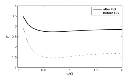
Figure 5: Entropy of entanglement of pure two-photon states described by Eqs. (71)–(74) before and after a 50/50 beam splitter as a function of the dimensionless pump width $\sigma/\Omega$.

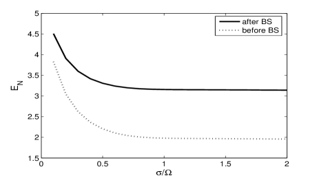
Figure 6: Logarithmic negativity of pure two-photon states described by Eqs. (71)–(74) before and after a 50/50 beam splitter as a function of the dimensionless pump width $\sigma/\Omega$.

Next we consider mixed two-photon states in a way that is similar to what we did for single photon states. We assume Gaussian wave packets with an uncertainty in arrival time. That is, we introduce a time-displaced mode function for two frequencies by

$$\psi(\omega,\omega^{\prime})\rightarrow\psi_{\tau}(\omega,\omega^{\prime})=\psi(\omega,\omega^{\prime})e^{-i(\omega+\omega^{\prime})\tau},$$ (84)

and we choose $P(\lambda)$ in Eq. (12) to take exactly the same form as Eq. (55) only that $\lambda$ is replaced by $\tau$. Since the Gaussian shape for $\tau$ falls off fairly quickly, we decided to extend the integral in our numerical calculations over the interval $(-2\sigma_{\tau},2\sigma_{\tau})$. To be more explicit, after the 50/50 beam splitter the mixed state looks like

$$\rho_{2{\rm out}} = \int d\tau P(\tau)|2_{\rm out}(\tau)\rangle\langle 2_{\rm out}(\tau)|,$$ (85)

where $P(\tau)\sim\exp(-\tau^{2}/\sigma^{2}_{\tau})$ and

$$|2_{\rm out}(\tau)\rangle=\frac{1}{2}\int d\nu_{o}\int d\nu_{e}\alpha_{\tau}(\nu_{o}+\nu_{e})\Phi(\nu_{o},\nu_{e})$$

$$\times e^{-i(\nu_{o}+\nu_{e})\tau}(c_{H}^{\dagger}(\nu_{o})c_{V}^{\dagger}(\nu_{e})+c_{V}^{\dagger}(\nu_{e})d_{H}^{\dagger}(\nu_{o})$$

$$-c_{H}^{\dagger}(\nu_{o})d_{V}^{\dagger}(\nu_{e})-d_{H}^{\dagger}(\nu_{o})d_{V}^{\dagger}(\nu_{e}))|{\rm v}\rangle.$$ (86)

By realizing that the two-photon states can be expanded in their own space $|2(\tau)\rangle_{c,d}$ instead of single-photon combination space, the size of the density matrix is greatly reduced from $(N+1)^{4}\times(N+1)^{4}$ to $(2N+T+1)^{2}\times(2N+T+1)^{2}$, $N$ and $T$ being the number of discretization intervals along $\omega$ and $\tau$ axes respectively.

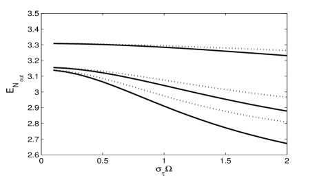
Figure 7: Logarithmic negativity of mixed two-photon states (85) –(86) after a 50/50 beam splitter vs. the dimensionless mixed-state width $\sigma_{\tau}\Omega$. The dotted curves are calculated by plugging the input state’s $E_{{\cal N}}$ into Eq. (82) and the solid curves are direct numerical results. Each set of dotted and solid curves has different wave packet width $\sigma$. From top to bottom: $\sigma/\Omega=0.5,1,2$.

Fig. 7 shows our numerical results regarding mixed two-photon states. We display two kinds of curves for three sets of parameters. The solid curves give the numerical results for $E_{{\cal N}}(\rho_{\rm out})$, whereas the dotted curves plot $2\log_{2}(1+2^{E_{{\cal N}}(\rho_{\rm in}\rangle)/2})$. In the case of a pure state these two quantities would be the same, according to (82), but for mixed states there is a small difference, indicating the relation (82) is a fair approximation for mixed states.

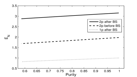
Figure 8: Logarithmic negativities of various mixed output states of a 50/50 beam splitter are plotted against purity. The single-photon result follows directly from Eq. (52), while the two-photon case is calculated from state Eq. (85). We have chosen $\sigma=\Omega$ for both two-photon states here and in all remaining figures.

From the preceding section we know the precise relation between entanglement generated by a beam splitter and purity for single-photon states. For comparison we plot in Fig. 8 the logarithmic negativity as a function of the purity of the mixed state for both single- and two- photon states. The almost linear behavior indicates the close relation between the characteristic purity of the system and the amount of entanglement that can be extracted under ideal conditions. Obviously, entanglement increases with purity.

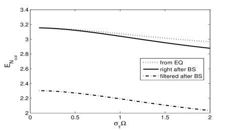
Figure 9: Logarithmic negativities for the output of mixed two-photon states (85)–(86). The dotted line is calculated from the relation Eq. (82), which is true for a pure state only. The dash-dotted line is the entanglement that would result after local filtering of the output state (see Section IV.3).

IV.2 Adding the vacuum

Type-II down conversion does not produce a two-photon state. Instead it produces a superposition of a two-photon state and the vacuum. Thus, let us first consider a pure state of the form

$$|{\rm vac2_{in}}\rangle=\sqrt{1-p}|{\rm v}\rangle+\sqrt{p}\sum_{k}\sqrt{\lambda_{k}}h_{k}^{\dagger}v_{k}^{\dagger}|{\rm v}\rangle,$$ (87)

where $p$ is the a priori probability to detect two photons, which typically will be small. In terms of the Schmidt coefficients we can easily calculate the entanglement present in the state (87),

$$E(|{\rm vac2_{in}}\rangle) = -(1-p)\log_{2}(1-p)-p\log_{2}p$$ (88)

$$-p\sum_{k}\lambda_{k}\log_{2}\lambda_{k},$$

$$E_{{\cal N}}(|{\rm vac2_{in}}\rangle) = 2\log_{2}(\sqrt{1-p}+\sqrt{p}\sum_{k}\sqrt{\lambda_{k}}).$$ (89)

Just as before we can express the entanglement of a state resulting from splitting this state on a 50/50 beam splitter in terms of the entanglement of the input state. The 50/50 beam splitter accordingly converts the state into

$$|{\rm vac2_{out}}\rangle = \sqrt{1-p}|0\rangle|_{c}0\rangle_{d}+\frac{\sqrt{p}}{2}(|\tilde{2}\rangle_{c}|0\rangle_{d}+|0\rangle_{c}|\tilde{2}\rangle_{d})$$ (90)

$$+\frac{\sqrt{p}}{2}\sum_{k}\sqrt{\lambda_{k}}(v_{ck}^{\dagger}h_{dk}^{\dagger}+h_{ck}^{\dagger}v_{dk}^{\dagger})|{\rm v}\rangle,$$

where $|\tilde{2}\rangle$ is given by Eq. (79). The entanglement measures are calculated to be

$$E(|{\rm vac2_{out}}\rangle)$$ (91)

$$= -\frac{1-p/2+\sqrt{1-p}}{2}\log_{2}\frac{1-p/2+\sqrt{1-p}}{2}$$

$$-\frac{1-p/2-\sqrt{1-p}}{2}\log_{2}\frac{1-p/2-\sqrt{1-p}}{2}$$

$$+p-\frac{p}{2}\log_{2}p-\frac{p}{2}\sum_{k}\lambda_{k}\log_{2}\lambda_{k},$$

$$E_{{\cal N}}(|{\rm vac2_{out}}\rangle)=2\log_{2}(1+\sqrt{p}\sum_{k}\sqrt{\lambda_{k}}).$$ (92)

We observe that

$$E_{\rm out}-\frac{1}{2}E_{\rm in}$$ (93)

$$= -\frac{1-p/2+\sqrt{1-p}}{2}\log_{2}\frac{1-p/2+\sqrt{1-p}}{2}$$

$$-\frac{1-p/2-\sqrt{1-p}}{2}\log_{2}\frac{1-p/2-\sqrt{1-p}}{2}$$

$$+\frac{1-p}{2}\log_{2}\left(\frac{1-p}{2}\right)+1,$$

and

$$2^{E_{{\cal N}{\rm out}}/2}-2^{E_{{\cal N}{\rm in}}/2}=1-\sqrt{1-p}.$$ (94)

These relations are the generalizations of Eq. (81) and Eq. (82) respectively when vacuum is involved.

For mixed states involving the vacuum no analytical results seem to be possible, so we reverted to numerical calculations. Fig. 10 plots some results from those calculations as a function of the probability $p$.

IV.3 Local filtering

The mixed two-photon state (85) is written as a mixture of pure two-photon states (86). The latter states are superpositions of two types of states: those with an odd number of photons in each output port of the beam splitter (namely, one), and those with an even number (namely, zero or two). By imagining performing a quantum nondemolition measurement of the parity of the photon number on (one of the) output ports, we are applying a local filter. This filtering cannot increase the entanglement and thus the entanglement after filtering gives a lower bound to the total entanglement present in the mixed state (85).

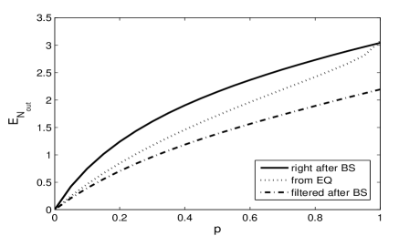
Figure 10: Logarithmic negativities for the output of a mixed two-photon state accompanied by vacuum at a fixed pump width $\sigma=\Omega$ and a mixture width $\sigma_{\tau}\Omega=1$. $p$ is the proportion of the two-photon state, as indicated in Eq. (87). The dotted line is calculated from the relation Eq. (92), which is true for a pure state only. The dash-dotted line is the entanglement after the beam splitter after the local filtering operation discussed in the text (Section IV.3).

In the pure-state case we can calculate the amount of entanglement resulting from filtering by collapsing the output Eq. (90) into either even-number-photon state

$$|\phi_{\rm even}\rangle=\frac{1}{\sqrt{1-p/2}}(\sqrt{1-p}|0\rangle|_{c}0\rangle_{d}$$

$$+\frac{\sqrt{p}}{2}|\tilde{2}\rangle_{c}|0\rangle_{d}+\frac{\sqrt{p}}{2}|0\rangle_{c}|\tilde{2}\rangle_{d})$$ (95)

with probability $1-p/2$ or the odd-number-photon state

$$|\phi_{\rm odd}\rangle=\frac{1}{\sqrt{2}}\sum_{k}\sqrt{\lambda_{k}}(v_{ck}^{\dagger}h_{dk}^{\dagger}+h_{ck}^{\dagger}v_{dk}^{\dagger})|{\rm v}\rangle$$ (96)

with probability $p/2$. Averaging the entanglement over the two possible measurement outcomes yields

$$E_{{\cal N}}^{\rm(even/odd)}$$ (97)

$$= (1-p/2)E_{{\cal N}}(|\phi_{\rm even}\rangle)+p/2E_{{\cal N}}(|\phi_{\rm odd}\rangle)$$

$$= p+p\log_{2}\sum_{k}\sqrt{\lambda_{k}}-\left(1-\frac{p}{2}\right)\log_{2}\left(1-\frac{p}{2}\right).$$

Figs. 9 and 10 illustrate this filtering effect for mixed states as a function of $\sigma_{\tau}\Omega$ for fixed $\sigma=\Omega$, and as a function of $p$ for fixed $\sigma$ and $\sigma_{\tau}$, respectively. One sees that about a third of the entanglement in the output state arises from coherence between states like $|1,1\rangle$ and $|0,2\rangle+|2,0\rangle$, in symbolic notation.

V Summary

We have quantified the entanglement of various mixed states containing exactly one or exactly two photons, as well as states with a nonzero vacuum component, by using the logarithmic negativity. For pure states we found simple relations between the entanglement of single-photon and two-photon states before and after a 50/50 beam splitter. For mixed states such relations are still found to be approximately true.

The simplest result arises for a mixed delocalized single photon. Its entanglement depends only on its purity. The result illustrates that even a perfect deterministic single-photon source (never producing more than a single photon) still may not be sufficient for certain quantum-information processing purposes (quantum computing based on dual-rail encoding, for example) if a large degree of entanglement is needed.

We considered fairly realistic cases by explicitly including a vacuum component of photon states, as well as including the spectral and/or temporal shapes of photon wave packets. But an obvious generalization of the present work would be to include full three-dimensional mode structures. Moreover, in the case of two photons impinging on a beam splitter we only treated the case of photons with orthogonal polarizations (having in mind type-II down conversion), but the similar case of identically-polarized photons is interesting as well, and, perhaps surprisingly, more complicated.

Appendix

Here we calculate explicitly the logarithmic negativity for the first example to show the entanglement of a color-mixed polarization-entangled state is still one ebit, in spite of the mixed nature of the state. The two-photon singlet state, maximally entangled in polarization — horizontal(H) or vertical(V) —, but equally and classically mixed in color — green(G) or blue(B)—, can be expressed in modes as

$$\rho=\frac{1}{2}|\phi_{1}\rangle\langle\phi_{1}|+\frac{1}{2}|\phi_{2}\rangle\langle\phi_{2}|,$$

where

$$|\phi_{1}\rangle=\frac{1}{\sqrt{2}}(|GH\rangle_{A}|GV\rangle_{B}-|GV\rangle_{A}|GH\rangle_{B}),$$

and

$$|\phi_{2}\rangle=\frac{1}{\sqrt{2}}(|BH\rangle_{A}|BV\rangle_{B}-|BV\rangle_{A}|BH\rangle_{B}).$$

Expanding $\rho$ in the basis of $(BH,BV)_{A}\otimes(BH,BV)_{B}\oplus(GH,GV)_{A}\otimes(GH,GV)_{B}$ gives

$$\rho=\left(\begin{array}[]{cc}\begin{array}[]{cccc}0&0&0&0\\ 0&\frac{1}{4}&-\frac{1}{4}&0\\ 0&-\frac{1}{4}&\frac{1}{4}&0\\ 0&0&0&0\\ \end{array}&0\\ 0&\begin{array}[]{cccc}0&0&0&0\\ 0&\frac{1}{4}&-\frac{1}{4}&0\\ 0&-\frac{1}{4}&\frac{1}{4}&0\\ 0&0&0&0\\ \end{array}\\ \end{array}\right).$$

The partial transpose of $\rho$ in the same basis is then

$$\rho^{\Gamma}=\left(\begin{array}[]{cc}\begin{array}[]{cccc}0&0&0&-\frac{1}{4}\\ 0&\frac{1}{4}&0&0\\ 0&0&\frac{1}{4}&0\\ -\frac{1}{4}&0&0&0\\ \end{array}&0\\ 0&\begin{array}[]{cccc}0&0&0&-\frac{1}{4}\\ 0&\frac{1}{4}&0&0\\ 0&0&\frac{1}{4}&0\\ -\frac{1}{4}&0&0&0\\ \end{array}\\ \end{array}\right).$$

The eight eigenvalues are easily found to be this: six times the eigenvalue $\frac{1}{4}$, and twice $-\frac{1}{4}$. This yields the logarithmic negativity of the state:

$$E_{\cal N}=\log_{2}(6\times\frac{1}{4}+2\times|-\frac{1}{4}|)=1,$$

as we announced.

References

• Ou and Mandel (1988) Z. Y. Ou and L. Mandel, Phys. Rev. Lett. 61, 50 (1988).
• Sergienko et al. (1995) A. V. Sergienko, Y. H. Shih, and M. Rubin, J. Opt. Soc. Am. B 12, 859 (1995).
• Kwiat et al. (1995) P. G. Kwiat, K. Mattle, H. Weinfurter, A. Zeilinger, A. V. Sergienko, and Y. Shih, Phys. Rev. Lett. 75, 4337 (1995).
• Kwiat et al. (1999) P. G. Kwiat, E. Waks, A. G. White, I. Appelbaum, and P. H. Eberhard, Phys. Rev. A 60, R773 (1999).
• U’Ren et al. (2005) A. B. U’Ren, C. Silberhorn, R. Erdmann, K. Banaszek, W. P. Grice, I. A. Walmsely, and M. G. Raymer, Las. Phys. 15, 146 (2005).
• Zanardi (2002) P. Zanardi, Phys. Rev. A 65, 042101 (2002).
• van Enk (2003) S. J. van Enk, Phys. Rev. A 67, 022303 (2003).
• Shi (2003) Y. Shi, Phys. Rev. A 67, 024301 (2003).
• Tan et al. (1991) S. M. Tan, D. F. Walls, and M. J. Collett, Phys. Rev. Lett. 66, 252 (1991).
• Hardy (1994) L. Hardy, Phys. Rev. Lett. 73, 2279 (1994).
• Babichev et al. (2004) S. A. Babichev, J. Appel, and A. I. Lvovsky, Phys. Rev. Lett. 92, 193601 (2004).
• Björk et al. (2001) G. Björk, P. Jonsson, and L. L. Sánchez-Soto, Phys. Rev. A 64, 042106 (2001).
• Hessmo et al. (2004) B. Hessmo, P. Usachev, H. Heydari, and G. Björk, Phys. Rev. Lett. 92, 180401 (2004).
• van Enk (2005) S. J. van Enk, Phys. Rev. A 72, 064306 (2005).
• Vidal and Werner (2002) G. Vidal and R. F. Werner, Phys. Rev. A 65, 032314 (2002).
• Plenio (2005) M. B. Plenio, Phys. Rev. Lett. 95, 090503 (2005).
• Grice and Walmsly (1997) W. P. Grice and I. A. Walmsly, Phys. Rev. A 56, 1627 (1997).
• Legero et al. (2006) T. Legero, T. Wilk, A. Kuhn, and G. Rempe, Adv. At. Mol. Opt. Phys. 53, 253 (2006).
• Raymer et al. (2005) M. G. Raymer, J. Noh, K. Banaszek, and I. A. Walmsley, Phys. Rev. A 72, 023825 (2005).
• Humble and Grice (2007) T. S. Humble and W. P. Grice, Physical Review A (Atomic, Molecular, and Optical Physics) 75, 022307 (2007).
• Humble and Grice (2008) T. S. Humble and W. P. Grice, Physical Review A (Atomic, Molecular, and Optical Physics) 77, 022312 (2008).
• Blow et al. (1990) K. J. Blow, R. Loudon, and S. J. D. Phoenix, Phys. Rev. A 42, 4102 (1990).
• Hong and Mandel (1985) C. K. Hong and L. Mandel, Phys. Rev. A 31, 2409 (1985).
• Ou et al. (1990) Z. Y. Ou, X. Y. Zou, L. J. Wang, and L. Mandel, Phys. Rev. A 42, 2957 (1990).
• Law et al. (2000) C. K. Law, I. A. Walmsley, and J. H. Eberly, Phys. Rev. Lett. 84, 5304 (2000).
• Parker et al. (2000) S. Parker, S. Bose, and M. B. Plenio, Phys. Rev. A 61, 032305 (2000).
• Spreeuw (2001) R. J. C. Spreeuw, Phys. Rev. A 63, 062302 (2001).
• Bennett et al. (1996) C. H. Bennett, D. P. DiVincenzo, J. A. Smolin, and W. K. Wootters, Phys. Rev. A 54, 3824 (1996).
• Lvovsky et al. (2007) A. I. Lvovsky, W. Wasilewski, and K. Banaszek, J. Mod. Opt. 54, 721 (2007).