Morphological evidence for azimuthal variations of the cosmic ray ion acceleration at the blast wave of SN 1006

Abstract

Using radio, X-ray and optical observations, we present evidence for morphological changes due to efficient cosmic ray ion acceleration in the structure of the southeastern region of the supernova remnant SN 1006. SN 1006 has an apparent bipolar morphology in both the radio and high-energy X-ray synchrotron emission. In the optical, the shock front is clearly traced by a filament of Balmer emission in the southeast. This optical emission enables us to trace the location of the blast wave (BW) even in places where the synchrotron emission from relativistic electrons is either absent or too weak to detect. The contact discontinuity (CD) is traced using images in the low-energy X-rays (oxygen band) which we argue reveals the distribution of shocked ejecta. We interpret the azimuthal variations of the ratio of radii between the BW and CD plus the X-ray and radio synchrotron emission at the BW using CR-modified hydrodynamic models. We assumed different azimuthal profiles for the injection rate of particles into the acceleration process, magnetic field and level of turbulence. We found that the observations are consistent with a model in which these parameters are all azimuthally varying, being largest in the brightest regions.

1 Introduction

Collisionless shocks in young supernova remnants (SNRs) are thought to be responsible for the production and acceleration of the bulk of Galactic cosmic rays (CRs) at least up to the “knee” ($\sim 3$ PeV) of the CR spectrum (e.g., Berezhko & Völk 2007). The theoretical mechanism is believed to be the first order Fermi acceleration, also known as diffusive shock acceleration (DSA), where electrons, protons and other ions scatter back and forth on magnetic fluctuations or Alfvén wave turbulence through the velocity discontinuity associated with the shock (Jones & Ellison 1991; Malkov & O’C Drury 2001, and references therein). The presence of the turbulence is a key ingredient in the process. The higher the turbulence level, the higher the scattering rate and the faster the acceleration proceeds, allowing particles to reach higher energies. The fast acceleration implies also that the CR pressure becomes significant very quickly so that the shock structure is highly nonlinear (e.g., Ellison et al. 2000; Baring 2007). The back-reaction of the particles on the shock hydrodynamics increases the level of magnetic turbulence and the injection rate in turn, i.e., the accelerated particles create the scattering environment by themselves (Bell 1978; Blandford & Ostriker 1978; Völk et al. 2003). Moreover, the production of relativistic particles (extracted from the thermal plasma) along with their escape from the shock system increases the overall density compression ratio (Berezhko & Ellison 1999; Blasi 2002).

This theoretical picture leads to several observational consequences. The intensity of the synchrotron emission from shock-accelerated electrons will be larger as the acceleration becomes more efficient since both the number of relativistic particles and intensity of the magnetic field must increase. In the region of very efficient acceleration, the X-ray synchrotron emission from the highest energy electrons will be concentrated in the form of thin sheets behind the blast wave due to synchrotron cooling in the high turbulent magnetic field amplified at the shock whereas the radio synchrotron emission will be much broader in comparison (Ellison & Cassam-Chenaï 2005). Finally, the morphology of the interaction region between the blast wave (BW) and the ejecta interface or contact discontinuity (CD) will become much thinner geometrically as the acceleration becomes more efficient due to the change in the compressibility of the plasma (Decourchelle et al. 2000; Ellison et al. 2004). Because shocks are believed to put far more energy into ions than electrons, this last point, if observed, would provide direct evidence for the acceleration of CR ions at the BW.

The detection of $\gamma$-rays with a neutral pion-decay signature resulting from the interaction of shock-accelerated protons with the ambient matter would provide evidence for CR ion acceleration as well. The best chance to see a clear pion-decay signal is when a SNR interacts with a dense medium, the prototype case being RX J1713.7–3946 (Cassam-Chenaï et al. 2004). Very high energy $\gamma$-rays have been detected from this remnant (Aharonian et al. 2007a) and also from a few others (e.g., Aharonian et al. 2007b; Hoppe et al. 2007). However, the pion-decay signal is generally difficult to extract from these observations because there are other processes efficiently producing $\gamma$-rays but involving CR electrons, namely bremsstrahlung and Inverse-Compton scattering off the 2.7 K cosmic microwave background and Galactic photons. The nature of the underlying process leading to $\gamma$-rays and therefore the nature of the emissive particles is subject to intense debate (e.g., Berezhko & Völk 2006; Porter et al. 2006; Uchiyama et al. 2007; Plaga 2008). Besides, in a large number of SNRs where bright and geometrically thin X-ray synchrotron-emitting rims are observed (e.g., Keper, Tycho, SN 1006), ambient densities are often very low leaving open the question of CR ion production in these SNRs (see also Katz & Waxman 2008).

The idea that the gap between the BW and CD allows quantifying the efficiency of CR ion acceleration was proposed by Decourchelle (2005) in the case of Tycho, Kepler and Cas A. In Tycho, a remnant where thin X-ray synchrotron-emitting rims are observed all around with little variations in brightness, Warren et al. (2005) showed that the BW and CD are so close to each other that they cannot be described by standard hydrodynamical models (i.e., with no CR component), hence providing evidence for efficient CR ion acceleration in this SNR. In a later study, Cassam-Chenaï et al. (2007) showed that the X-ray and to some extent the radio properties of the synchrotron emitting rim as well as the gap between the CD and BW were consistent with efficient CR ion acceleration modifying the hydrodynamical evolution of Tycho.

Ideally, one would like to find a SNR where both efficient and inefficient particle acceleration take place so that differential measurements can be made. This offers a great advantage for the astrophysical interpretation since a number of uncertainties (e.g., distance and age) can be eliminated in the comparison. Furthermore, by directly observing a difference in the gap between the BW and CD in regions of efficient and inefficient acceleration, one obtains a direct, model-independent, confirmation that CRs do indeed modify the hydrodynamical evolution of the BW. SN 1006 provides a valuable laboratory in that regard since the gradual variations of the intensity of the radio and X-ray synchrotron emission along the BW point to underlying variation of CR ion acceleration. The task of measuring the ratio of radii between the BW and CD in the regions of inefficient and efficient CR acceleration will be challenging. Nonetheless, SN 1006 is one of the rare objects (perhaps even the unique one) where this can be accomplished as we explain below.

In this paper, we focus our attention on the poorly studied southeastern (SE) quadrant of SN 1006, i.e., along the shock front lying between the northeastern and the southwestern synchrotron-emitting caps. Our first goal is to measure the ratio of radii between the BW and CD there. We can fairly easily follow the BW in the bright synchrotron-emitting caps (presumably the regions of efficient CR acceleration) and the BW can still be traced from the H$\alpha$ emission in the region where both the radio and X-ray synchrotron emissions are either too faint to be detected or absent (presumably the regions of inefficient CR acceleration). As for the CD, it can be traced from the thermal X-ray emission associated with the shocked ejecta. Our second objective is to measure the azimuthal variations of the synchrotron brightness in the radio and several X-ray energy bands. With these observational key results in hand, we use CR-modified hydrodynamic models of SNR evolution to constrain the azimuthal variations of the acceleration parameters, i.e., the injection rate of particles in the acceleration process, strength of the magnetic field, particle diffusion coefficient and maximum energy of electrons and ions.

This paper is organized as followed. In §2, we describe the basic characteristics of SN 1006. In §3, we present the data used in our study. In §4, we present the key observational results in SN 1006. In §5, we try to relate hydrodynamical models with those results in the context of CR-unmodified and -modified shocks. Finally, we discuss our results (§6) and present our conclusion (§7).

2 Basic characteristics of SN 1006

SN 1006 was a thermonuclear supernova (SN) widely seen on Earth in the year 1006 AD. More than a thousand year later, the remnant from this explosion is a huge shell of $30\arcmin$ angular size.

The synchrotron emission is detected from the radio up to the X-rays and dominates in two bright limbs – the northeast (NE) and southwest (SW) – where several thin ($20\arcsec$ width or so) rims/arcs are running at the periphery, sometimes crossing each other (Bamba et al. 2003; Long et al. 2003; Rothenflug et al. 2004). Those apparent ripples are most likely the result of the projection of undulating sheets associated with the shock front. The radio emission is well correlated with the nonthermal X-rays (Reynolds & Gilmore 1986; Long et al. 2003). Both show an abrupt turn-on with coincident edges in the radial directions, but the X-ray emission has more pronounced narrow peaks. This points to a scenario in which the rims are limited by the radiative losses in a highly turbulent and amplified magnetic field (Berezhko et al. 2002, 2003; Ellison & Cassam-Chenaï 2005; Ballet 2006). Finally, the observed synchrotron morphology in SN 1006 is best explained if the bright limbs are polar caps with the ambient magnetic field parallel to the shock velocity (Rothenflug et al. 2004). In the caps, the maximum energy reached by the accelerated particles, as well as their number, must be higher than elsewhere (Rothenflug et al. 2004).

In contrast to the nonthermal X-ray emission, the very faint thermal X-ray emission seems to be distributed more or less uniformly (Rothenflug et al. 2004). This is best seen in the oxygen band (0.5-0.8 keV). It is, however, difficult to separate the thermal emission from the nonthermal emission in the caps. Moreover, it is not clear whether the thermal X-rays should be attributed to the shocked ambient medium (Yamaguchi et al. 2007) or the shocked ejecta (Long et al. 2003), but both the over-solar abundances required to fit the X-ray spectra in the inner northwest (NW) and NE parts of the SNR and the clumpiness on a $30\arcsec$ to $1\arcmin$ scale of the low-energy X-ray emission favor an ejecta origin. The SE region seems to be slightly different than the rest of the SNR in terms of ejecta composition and clumpiness too. There is, in particular, evidence for the presence of cold (Winkler et al. 2005) and reverse-shock heated (Yamaguchi et al. 2007) iron. In terms of dynamics, there is evidence for ejecta extending to/overtaking the BW in the NW (Long et al. 2003; Vink et al. 2003; Raymond et al. 2007).

In the optical, the remnant has a very different morphology. Deep H$\alpha$ imaging reveals very faint Balmer emission around almost the entire periphery with a clear arc or shock front running from east to south (Winkler & Long 1997; Winkler et al. 2003). Interestingly, no synchrotron emission is detected in X-ray in this southeast (SE) region whereas extremely faint (and highly polarized) synchrotron emission is detected in the radio (Reynolds & Gilmore 1993). Besides, none of the optical emission is of synchrotron origin. There is also a clear Balmer line filament in the NW of SN 1006 which has been observed in great detail in the optical (Ghavamian et al. 2002; Sollerman et al. 2003; Raymond et al. 2007), ultraviolet (Raymond et al. 1995; Korreck et al. 2004; Hamilton et al. 2007) and X-ray bands (Long et al. 2003; Vink et al. 2003; Acero et al. 2007), providing diagnostics for the shock speed ($V_{s}\sim 2400-3000\>\mathrm{km/s}$), ion-electron thermal equilibration at the shock ($T_{e}/T_{p}\leq 0.07$) and preshock ambient density ($0.25\>\mathrm{cm}^{-3}\leq n_{0}\leq 0.4\>\mathrm{cm}^{-3}$). Optical proper motions (Winkler et al. 2003) combined with the shock speed estimate (Ghavamian et al. 2002; Heng & McCray 2007) along this NW filament leads to a distance to the SNR between $1.8$ and $2.3$ kpc. However, because the remnant is interacting with a denser medium in the NW (Moffett et al. 1993; Dubner et al. 2002), the shock speed and the ambient density, in particular, might be respectively higher and lower elsewhere (Acero et al. 2007). For instance, the broadening of the oxygen (Vink et al. 2003) and silicon (Yamaguchi et al. 2007) X-ray emission-lines suggest a shock speed $V_{s}\geq 4000\>\mathrm{km/s}$ (although these measurements were carried out at different locations in SN 1006). Such high velocities are compatible with recent proper motion measurements based on radio data (Moffett et al. 2004; Reynoso et al. 2008). Moreover, the lack of observed TeV $\gamma$-ray emission (Aharonian et al. 2005) sets an upper limit on the ambient density of $n_{0}\leq 0.1\>\mathrm{cm}^{-3}$ (Ksenofontov et al. 2005) and the high latitude ($\sim 500\>\mathrm{pc}$ at a distance of $2$ kpc) of SN 1006 suggests that $n_{0}\sim 0.03-0.04\>\mathrm{cm}^{-3}$ (Ferrière 2001).

3 Data

3.1 X-ray

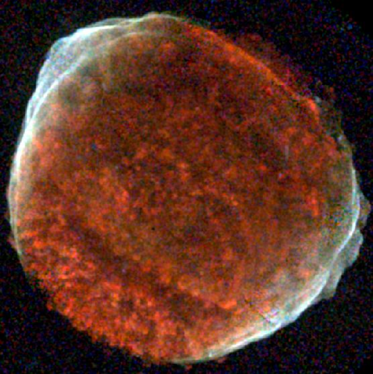
Figure 1: Three-color Chandra image of SN 1006: 0.5-0.8 keV (red), 0.8-2 keV (green) and 2-4.5 keV (blue). The regions dominated by synchrotron emission from high-energy relativistic electrons appears in white and are naturally associated with the BW. The regions dominated by the thermal emission from the shocked gas (mostly oxygen) appears in red and are most likely associated with the ejecta. Note that the oxygen is found slightly ahead of the BW in some places (e.g., east and south). Point sources have been removed here so that only the diffuse emission from the remnant is visible. Images were background subtracted, corrected for vignetting and slightly smoothed. The intensity scaling is square-root with a maximum fixed at $5.0\times 10^{-4}$, $5.0\times 10^{-4}$ and $2.0\times 10^{-4}$ ph/cm²/s/arcmin² for the red, green and blue bands, respectively.

We used the most recent Chandra data of SN 1006 (ObsId 3838 and ObsId 4385 up to 4394) which were obtained in April 2003 with the ACIS-I imaging spectrometer in timed exposure and very faint data modes. Eleven pointings were necessary to cover the entire extent of the remnant. The final image is shown in Figure 1. The X-ray analysis was done using CIAO software (ver. 3.4). Standard data reduction methods were applied for event filtering, flare rejection, gain correction. The final exposure time amounts to $\sim 20$ ks per pointing.

3.2 Radio

Radio observations were performed in 2003 (nearly at the same time as the X-ray observations) with both the Australia Telescope Compact Array (ATCA) and the Very Large Array (VLA).

The ATCA consists of an array of six 22-m antennae that attain a maximum baseline of 6 km in the East-West direction. The ATCA observations occurred on three separate occasions in antenna configurations that optimize high spatial resolution: January 24 in its 6-km B configuration for 12 hours, March 3 in its 6-km A configuration for 12 hours, and June 12 in its 750-m C configuration for 7 hours. Observations were made using two 128-MHz bands (divided into 32 channels each) centered at 1384 and 1704 MHz. The source PKS 1934–638 was used for flux density and bandpass calibration, while PKS 1458–391 was used as a phase calibrator. The total integration time on SN 1006 was over 1500 minutes.

The VLA consists of 27 25-m antennae arranged in a “Y” pattern. Observations with the VLA were carried out during 4 hours on January 25th in its hybrid CnD configuration (arranged to maximize spatial resolution when observing southern declination sources). Observations were made using two 12.5-MHz channels centered at 1370 and 1665 MHz. 3C286 and 1451–400 were observed for flux and phase calibration. The total VLA integration time on SN 1006 was 140 minutes.

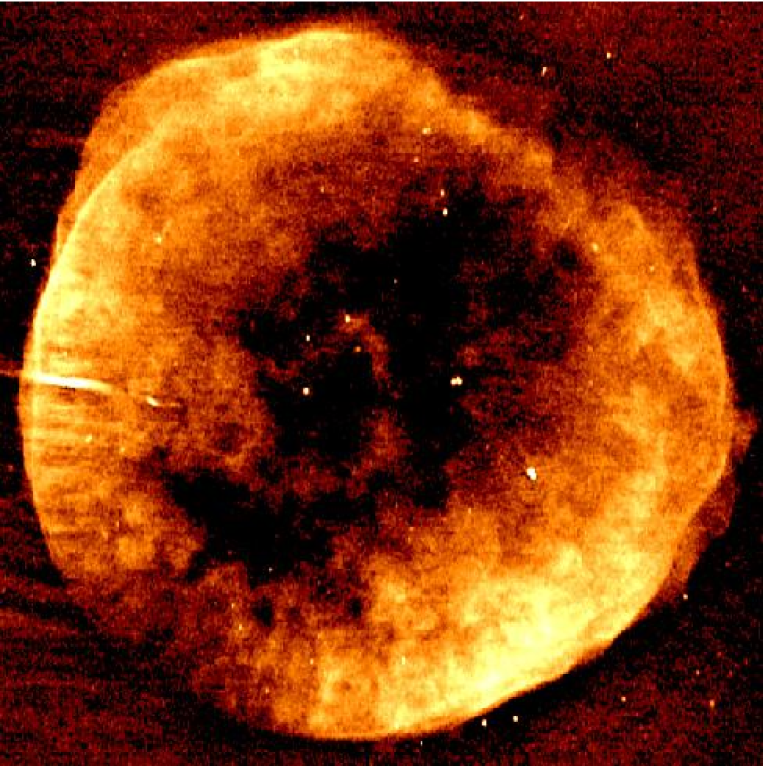
Figure 2: Radio image of SN 1006 at 1.5 GHz. The intensity scaling is square-root with a maximum fixed at $1.0$ mJy$/$beam. The bright elongated source in the western rim is a background radio galaxy.

Data from all of the observations were combined, then uniformly weighted during imaging to minimize the effects of interferometric sidelobes. The final image, shown in Figure 2, has a resolution of $\sim 6\arcsec\times 9\arcsec$ and an off-source rms noise of $20\>\mu\mathrm{Jy/beam}$ near the rims. Since the angular size of SN 1006 is comparable to the primary beam of both instruments (half a degree), corrections were applied to the image to recover the lost flux. After primary beam corrections, the total flux density was recovered to within $<5\%$ of the expected value. With primary beam correction, noise increases in the faint SE portion. For the study of the azimuthal variations of the radio emission at the shock, we use non beam corrected data (§4.2).

3.3 Optical

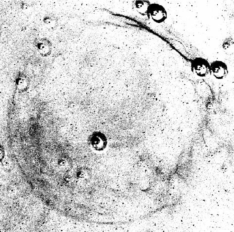
Figure 3: H$\alpha$ image of SN 1006.

We used the very deep H$\alpha$ image presented by Winkler et al. (2003). This image taken in June 1998, that is 5 years before the X-ray data, is shown in Figure 3. To compare the optical and X-ray images, we had to correct for the remnant’s expansion. In the optical, proper motions of $0.280\pm 0.008\>\arcsec\>\mathrm{yr}^{-1}$ were measured (from April 1987 to June 1998) along the NW rim where thin nonradiative Balmer-dominated filaments are seen (Winkler et al. 2003). In the radio, an overall expansion rate of $0.44\pm 0.13\>\arcsec\>\mathrm{yr}^{-1}$ was measured (from May 1983 to July 1992, Moffett et al. 1993), although higher values have been measured using more recent observations (Moffett et al. 2004; Reynoso et al. 2008). This value does not include the NW rim where the optical filaments are observed because there is simply little or no radio emission there. The observed expansion rate is clearly higher in the radio than in the optical and is consistent with the picture in which the BW encounters a localized and relatively dense medium in the NW. For simplicity, when using radial profiles, we use the value of $0.40\arcsec\>\mathrm{yr}^{-1}$, so that the optical profiles are shifted by $2\arcsec$ to be compared with the X-ray profiles. As we show below, this correction is negligible compared to other uncertainties when trying to locate the fluid discontinuities.

4 Key observational results

4.1 Fluid discontinuities

In this section, we determine the location of the fluid discontinuities – i.e., the BW and CD – in the SE quadrant of SN 1006. Our goal is to measure the gap between the BW and CD as a function of azimuth.

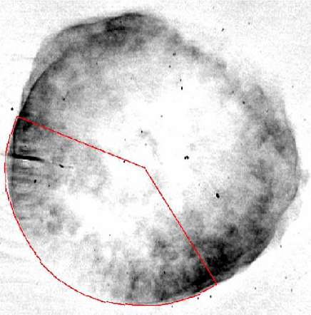
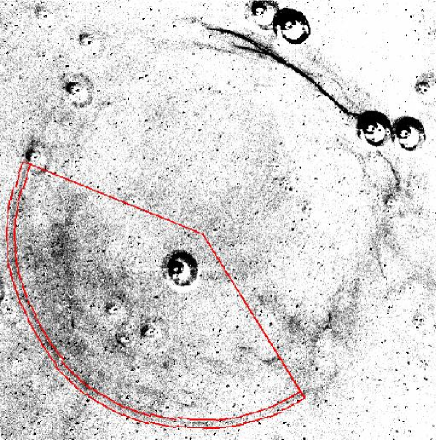
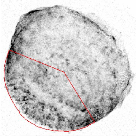
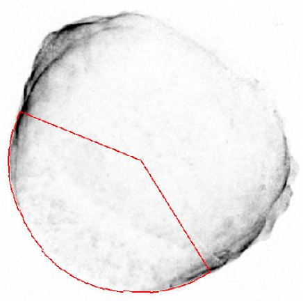
Figure 4: Images of SN 1006 in several energy bands. Top-left: Radio image at 1.5 GHz. The maximum intensity was fixed at $0.6$ mJy$/$beam. Top-right: H$\alpha$ image with the contour errors associated with the shock front seen in the southeast (red lines). Bottom-left: Chandra X-ray image in the oxygen band (0.5-0.8 keV). The maximum intensity was fixed at $5.0\times 10^{-4}$ ph/cm²/s/arcmin². Bottom-right: Chandra image in the mid-energy X-ray band (0.8-2.0 keV). The maximum intensity was fixed at $6.0\times 10^{-4}$ ph/cm²/s/arcmin². Both X-ray images were background subtracted, corrected for vignetting and slightly smoothed. In the radio and X-ray images, we show the contour derived from the H$\alpha$ emission (red lines). This contour lies within the contour errors shown in the H$\alpha$ image. In all the images, the intensity scaling is linear.

To trace the location of the BW, we use the H$\alpha$ image of SN 1006 which shows very faint filaments of Balmer emission around much of the periphery of the remnant (Fig. 4, top-right panel). In the southeastern quadrant, the H$\alpha$ emission follows a nearly circular arc. We extracted radial profiles by azimuthally summing over $4^{\circ}$ wide sectors starting from $158^{\circ}$ (from west) to $302^{\circ}$ (in the clockwise direction). The center of these profiles was determined to provide the best match to the curvature of the H$\alpha$ rim. The coordinates of the center are $(\alpha_{\mathrm{J2000}},\delta_{\mathrm{J2000}})=(15^{\mathrm{h}}02^{\mathrm{m}}56.8^{\mathrm{s}},-41^{\circ}56\arcmin 56.6\arcsec)$. This center is very close to the geometrical center of the SNR, which, given its overall circularity, may not be too far from the overall expansion center which has not yet been determined. In practice we found it very difficult to determine the location of the optical rim based purely on a numerical value (e.g., contour value or enhancement factor above the local background level) because of the presence of faint stellar emission, poorly subtracted stars, and faint diffuse H$\alpha$ emission across the image. So, we identified locations where the H$\alpha$ emission increased slightly in the radial profiles by eye and then further checked (again visually) the corresponding radii on the optical image. We associated generous uncertainties with the radii derived from this procedure: $12\arcsec$ outward and $24\arcsec$ inward (our process tended to overestimate the radii, hence the asymmetric errors).

To trace the location of the CD, we use the X-ray image in the low-energy band ($0.5-0.8$ keV) which contains most of the oxygen lines (Fig. 4, bottom-left panel). While it is not clear whether the oxygen emission comes from the shocked ambient medium or the shocked ejecta, we consider here an ejecta origin. We discuss and justify this assumption below (§5.1). Another issue comes from the fact that the X-ray emission in the oxygen band may contain some nonthermal contribution in the bright limbs. The three-color composite X-ray image (Fig. 1) reveals that the oxygen emission (red color) is in fact fairly different from the nonthermal X-rays (white color), and appears notably clumpier even in the synchrotron limbs (see the eastern limb for instance). This tells us that we can still use the oxygen emission to trace the CD in the bright limbs, at least in the azimuthal range we selected ($158^{\circ}-302^{\circ}$) where the synchrotron emission is not completely overwhelming. Radial profiles were extracted from a flux image, summing over $1^{\circ}$ wide sectors, with the same center and azimuthal range as for the optical. In the radial profiles, we selected the radii for which the brightness becomes larger than $1.5\times 10^{-5}$ ph/cm²/s/arcmin².

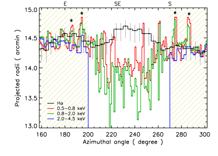
Figure 5: Azimuthal variation of the outer H$\alpha$ emission (black lines) and X-ray emission as obtained in several X-ray energy bands: 0.5-0.8 keV (red lines), 0.8-2 keV (green lines) and 2-4.5 keV (blue lines). Regions where the X-ray synchrotron emission is dominant are indicated by cross-hatched yellow lines. In those regions, the fingers (stars) indicate the presence of shocked ejecta found at or even slightly ahead of the BW. The X-ray contours correspond to places where the brightness becomes larger than $1.5\times 10^{-5}$ ph/cm²/s/arcmin² in the $0.5-0.8$ keV band, $0.6\times 10^{-5}$ ph/cm²/s/arcmin² in the $0.8-2$ keV band and $0.4\times 10^{-5}$ ph/cm²/s/arcmin² in the $2-4.5$ keV band. Note that the radii measurements are quite sensitive to the contour values, but the range of variations is contained between the red and blue lines.

Figure 5 summarizes the above-described measurements and shows the azimuthal variations of the radii as determined from the H$\alpha$ emission (black lines) and low-energy ($0.5-0.8$ keV, red lines), mid-energy ($0.8-2.0$ keV, green lines) and high-energy ($2.0-4.5$ keV, blue lines) X-ray emissions. The cross-hatched lines indicate the location of the bright synchrotron limbs. They correspond to the places where the contour of the outer high-energy X-ray emission (blue lines) can be determined. Between the two synchrotron caps (angles between $200^{\circ}$ and $270^{\circ}$), there is a clear gap between the BW and CD which is easily seen in Figure 4 (bottom-left panel). In the bright limbs, however, the BW and CD are apparently globally coincident. Fingers of ejecta (indicated by the stars) are even sometimes visible clearly ahead of the H$\alpha$ emission. In these places, the H$\alpha$ emission might not be the best tracer of the BW location. The mid-energy X-ray emission (green lines) shows that these fingers are also present. It is not clear whether this emission traces the BW or, again, the ejecta (mostly silicon). The high-energy X-ray emission (blue lines) cannot be used, nor a X-ray spectral analysis, to answer this point because of the low number of X-ray counts in this region.

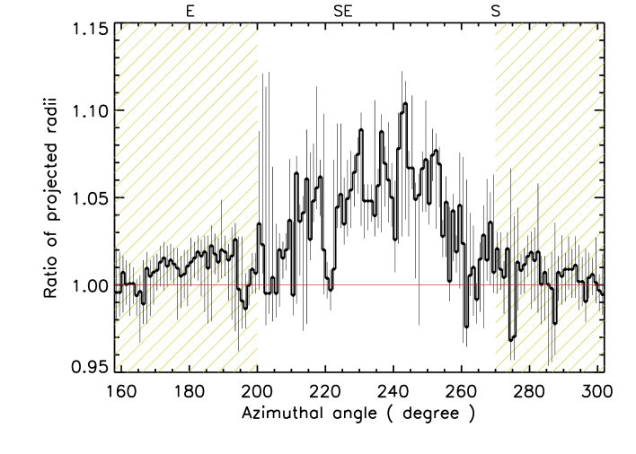
Figure 6: Ratio of the outer H$\alpha$ radius (black lines in Fig. 5) to the 0.5-0.8 keV X-ray radius (red lines in Fig. 5). Regions where the X-ray synchrotron emission is dominant are indicated by cross-hatched yellow lines. Error bars include uncertainties on the radius derived from the (expanded) H$\alpha$ image and that done in the low-energy X-rays choosing different contour values ($2.5\pm 1.0\times 10^{-5}$ ph/cm²/s/arcmin²). The large error bars between $200^{\circ}-205^{\circ}$ are due to a low exposure there.

Figure 6 shows the ratio of radii for the H$\alpha$ and low-energy X-ray emission, which to first approximation corresponds to the ratio of radii between the BW and CD, $R_{\rm BW}/R_{\rm CD}$. With increasing azimuthal angles the ratio of radii increases from values near unity (within the northeastern synchrotron-emitting cap) to a maximum of $R_{\mathrm{BW}}/R_{\mathrm{CD}}\simeq 1.10^{+0.02}_{-0.04}$ before falling again to values near unity (in the southwestern synchrotron-emitting cap). Over the entire azimuthal region where the synchrotron emission is faint, the azimuthally averaged ratio of radii is $R_{\rm BW}/R_{\rm CD}\simeq 1.04\pm 0.03$. In the regions within the synchrotron rims, $R_{\rm BW}/R_{\rm CD}\simeq 1.00$.

4.2 Synchrotron emission at the blast wave

In this section, we measure the azimuthal variations of the synchrotron flux extracted at the BW and we investigate how these variations compare when measured at different frequencies.

For that purpose, we use radio and X-ray data (Fig. 4, left panels). We extracted the flux in a $30\arcsec$-wide region behind the BW along the SE rim. To define the BW location, we used the well-defined radii obtained from the high-energy X-ray image for the northeastern ($\theta\leq 200^{\circ}$) and southwestern ($\theta\geq 270^{\circ}$) regions while, in the remaining SE quadrant ($200^{\circ}<\theta<270^{\circ}$), we used the radii determined from the H$\alpha$ image since no synchrotron emission is detected there.

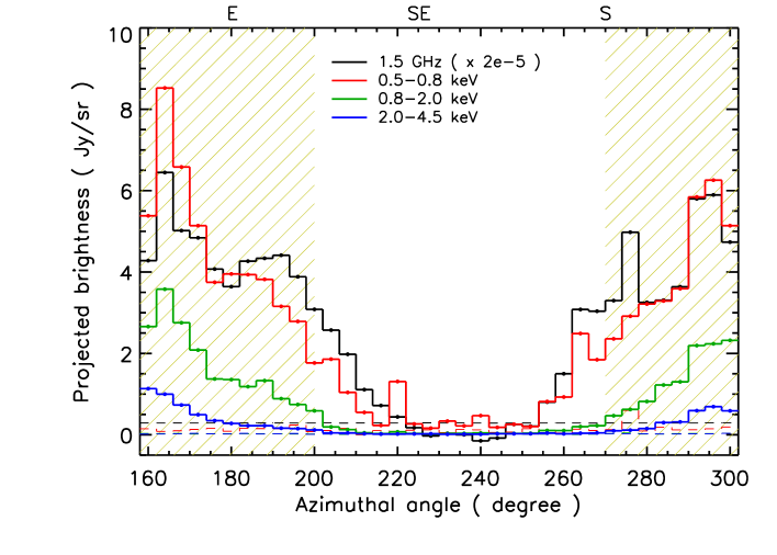
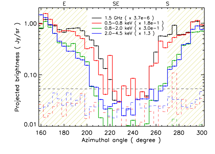
Figure 7: Top: Azimuthal variations of the brightness at the BW of SN 1006 at several frequencies/energies: 1.5 GHz (black lines), 0.5-0.8 keV (red lines), 0.8-2 keV (green lines) and 2-4.5 keV (blue lines). The brightness in each azimuthal bin was calculated between the BW radius and the radius $30\arcsec$ behind. For comparison, we show the level of the radio rms noise level and X-ray background located $1\arcmin$ outside the BW and extracted from a $30\arcsec$-wide box (dashed lines). Bottom: Same but with the curves rescaled roughly to the same level in the brightest regions and shown with a log scale.

In Figure 7 (top panel), we show the azimuthal variations of the projected brightness in the radio (1.5 GHz, black lines), and several X-ray energy bands: $0.5-0.8$ keV (red lines), $0.8-2.0$ keV (green lines) and $2.0-4.5$ keV (blue lines). The radio brightness was multiplied by $2\times 10^{-5}$ to make it appear on the same plot with the X-ray data. When moving from the northeastern or southwestern synchrotron-emitting caps toward the faint SE region, we see that the projected brightness gradually decreases in both radio and X-ray bands. The radio, medium- (green lines) and high-energy (blue lines) X-rays show mostly the variations of the synchrotron emission, while the low-energy X-rays (red lines) show mostly the variations of the thermal (oxygen) emission, but may contain some nonthermal contribution as well.

In Figure 7 (bottom panel), we show the same azimuthal variations but rescaled roughly to the same level in the synchrotron-emitting caps. The logarithmic scale shows that the brightness contrast between the bright caps and faint SE region is of order $20$ to $50$ in the radio and X-rays. In fact, this value might even be larger since the radio and high-energy X-ray fluxes in the faint SE quadrant are compatible with no emission. We note that the azimuthal variations of the radio synchrotron emission are much less pronounced than those in the X-rays.

5 Relating hydrodynamical models to the observations

In the previous section, we have found evidence for azimuthal variations of the separation between the BW and CD and synchrotron brightness just behind the BW (§4). Both the separation and the brightness are correlated: the brighter the BW, the smaller the separation. We measured in particular an unexpectedly small separation between the BW and CD ($\sim 1.04$) in the SE quadrant of SN 1006 where little to no synchrotron emission is detected. These measurements depend on the assumption that the oxygen emission comes from the shocked ejecta. After justifying this approach below (§5.1), we first investigate the different scenarios that could potentially lead to a small ratio of radii between the BW and CD assuming no CR acceleration at the shock (§5.2). Finally, we interpret the observed azimuthal variations of the ratio of radii and synchrotron brightness using CR-modified hydrodynamic models (§5.3).

5.1 Does the oxygen come from the ejecta?

A strong assumption made in the measurement of the ratio of radii between the BW and CD in SN 1006 is that the thermal X-ray emission (from the oxygen) is associated with the shocked ejecta.

There is, however, still the possibility that the oxygen emission is associated with the shocked ambient medium. Yamaguchi et al. (2007) have shown that the integrated X-ray spectrum of the SE quadrant can be described by a combination of three thermal plasmas in non-equilibrium ionization and one power-law component. One of the thermal components, assumed to have solar abundances and therefore associated with the shocked ambient medium, was able to produce most of the observed low-energy X-rays (in particular the K$\alpha$ lines from O vii, O viii and Ne ix). The two other thermal components, with non-solar abundances, were able to reproduce most of the K$\alpha$ lines of Si, S and Fe, and were attributed to the shocked ejecta.

There are several arguments from an examination of the high resolution Chandra images, however, that favor an ejecta origin for the low-energy X-ray emission. The three-color composite X-ray image (Fig. 1) shows that the spectral character of the X-ray emission in the SE quadrant (where there is little to no synchrotron emission) does not change appreciably as a function of radius behind the BW, which would be expected if the Yamaguchi et al. (2007) picture were correct. The lack of virtually any X-ray emission between the BW and CD can be explained by the expected low density of the ambient medium ($\sim 0.03-0.04$ cm^-3 Ferrière 2001) which can reduce both the overall intensity and the level of line emission (due to strong nonequilibrium ionization effects). If the soft X-ray emission were from the shocked ambient medium its brightness should in principle rise gradually behind the BW as a result of the projection of a thick shell onto the line-of-sight (Warren et al. 2005), but the radial profile of the low-energy X-ray emission (not shown) in fact turns on rather quickly at the periphery.

Another argument in favor of an ejecta origin is the observed clumpiness of the oxygen emission throughout the SE region. There is also the protuberances seen right at the edge of SN 1006, which are suggestive of Rayleigh-Taylor hydrodynamical instabilities that are expected at the CD (see Fig. 1). Note that the outer edge of the long, thin filament of X-ray emission in the NW – which overlaps the brightest H$\alpha$ emission and therefore is likely to be at least partly due to shocked ambient medium – is much smoother than the edge of the remnant in the SE. Finally, high emission measures of oxygen in the shocked ejecta at young dynamical SNR ages are compatible with most thermonuclear explosion models. Essentially, all 1-D and 3-D deflagration models, and all delayed detonation and pulsating delayed detonation models have oxygen in the outer layers (but not prompt detonations or sub-Chandrasekhar explosions) (Badenes et al. 2003).

5.2 The small gap in the faint SE region

We have presented evidence in §4.1 for a small ratio of radii $R_{\mathrm{BW}}/R_{\mathrm{CD}}\sim 1.04$ between the BW and CD in the SE quadrant of SN 1006. This is also the location where the radio and X-ray nonthermal emission are either very weak or undetected. The most straightforward explanation for this lack of synchrotron emission is an absence of efficient CR acceleration at the BW here. In the following sections, we first investigate whether pure 1-D hydrodynamical models for SNR evolution (i.e., without CR acceleration) can reproduce such a small ratio of radii. We consider the role of ambient density, ejecta profile, and explosion energy on the size of the gap between CD and BW. Then we consider the effects of 3-D projection on the hydrodynamically unstable CD.

5.2.1 Predictions from standard hydrodynamical models

To understand how a small gap can be produced in a region where there is apparently no evidence for efficient particle acceleration, we used standard one dimensional (1-D) spherically symmetric numerical hydrodynamical simulations that follow the interaction of the ejecta with the ambient medium. These simulations do not include any CR component.

Key inputs to these simulations are the initial density profiles of the ejecta and ambient medium. In the following, we consider a uniform density in the ambient medium and two different initial ejecta density profiles: exponential and power-law. The exponential form has been shown to be most representative of explosion models for thermonuclear SNe (Dwarkadas & Chevalier 1998), but we also present results with a power-law distribution to quantify the impact of the shape or compactness of the ejecta profile on $R_{\mathrm{BW}}/R_{\mathrm{CD}}$.

In general, an exponential profile is expected for thermonuclear SNe because the explosion is driven by the continuous release of energy from the burning front as it propagates through the star, while the power-law profile (more compact) is expected for core collapse SNe because the explosion is driven by a central engine (core bounce), and the shock loses energy as it propagates through the star (Matzner & McKee 1999). Power law profiles with $n=7$ have been used to represent 1-D deflagration models (in particular, model W7 from Nomoto et al. 1984), while exponential profiles are more adequate to represent delayed detonation models (Dwarkadas & Chevalier 1998). When comparing these two analytical profiles, it is worth noting that they transmit momentum to the ISM in a different manner. The more compact power law profile is a more efficient piston for ISM acceleration, and will lead to smaller gaps than the less compact exponential profile (Dwarkadas & Chevalier 1998; Badenes et al. 2003).

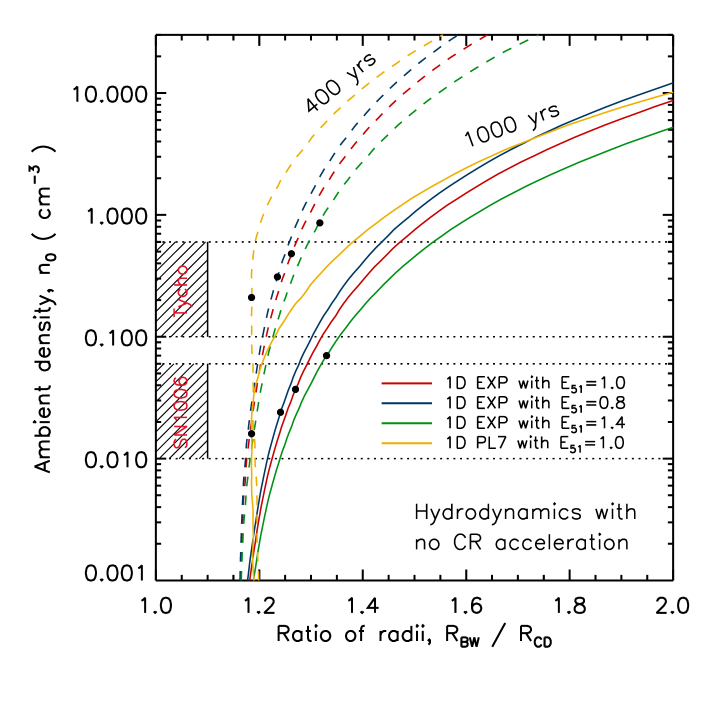
Figure 8: Ratio of radii between the BW and CD, $R_{\mathrm{BW}}/R_{\mathrm{CD}}$, as obtained from 1-D numerical hydrodynamical simulations (assuming no CR acceleration at the BW) and calculated for a large range of ambient density, $n_{0}$, for a fixed SNR age (dashed lines: 400 yrs; solid lines: 1000 yrs). We show curves obtained with a 1-D exponential (EXP) ejecta profile with a kinetic energy of the explosion $E_{51}\equiv E/10^{51}$ ergs $=1.0$ (red lines), $E_{51}=0.8$ (blue lines), $E_{51}=1.4$ (green lines) and a 1-D powerlaw (PL7) ejecta profile ($n=7$) with $E_{51}=1.0$ (yellow lines). The cross-hatched domains correspond to the intersection of the range of ratio of radii observed in SN 1006 and Tycho ($\leq 1.10$, vertical solid lines) and range of ambient medium density typically encountered in their vicinity (horizontal dotted lines). The 1-D hydrodynamical simulations are clearly unable to predict a ratio of radii as small as the one observed in both SNRs. For completeness, we indicate by a filled circle the value of the ambient density at which the simulated SNR radius matches the one observed for each model. An angular BW radius of $14.6\arcmin$ (resp. $256\arcsec$) and a distance to the SNR of $2.0$ kpc ($2.8$ kpc) were assumed for SN 1006 (resp. Tycho), resulting in a physical BW radius of $\sim 8.5$ pc (resp. $\sim 3.5$ pc). Larger values for the physical radius (due for instance to a larger distance to the remnant) would correspond to lower ambient densities.

The hydrodynamical simulations provide the radii of the BW and CD at any time for a given ejecta profile, ambient medium density, and explosion energy. In Figure 8, we quantify the impact of these three contributions on the ratio of radii $R_{\mathrm{BW}}/R_{\mathrm{CD}}$. In particular, we plot the ratio obtained for a wide range of ambient medium density ($0.001\>\mathrm{cm}^{-3}\leq n_{0}\leq 30\>\mathrm{cm}^{-3}$) using 1-D exponential (EXP) and powerlaw (PL7) ejecta profiles with different kinetic energies. The cross-hatched domains define the range of ratio of radii observed in SN 1006 and Tycho ($R_{\mathrm{BW}}/R_{\mathrm{CD}}\leq 1.10$) and range of typical ambient densities ($0.01\>\mathrm{cm}^{-3}\leq n_{0}\leq 0.06\>\mathrm{cm}^{-3}$ in SN 1006; $0.1\>\mathrm{cm}^{-3}\leq n_{0}\leq 0.6\>\mathrm{cm}^{-3}$ in Tycho) consistent with constraints derived from the observations (Acero et al. 2007; Cassam-Chenaï et al. 2007). It is clear that the 1-D hydrodynamical simulations are unable to reproduce a ratio of radii as small as the one observed in both SNRs. We note however that such a comparison between the observations and the models is not straightforward since our measurements are likely to be affected by projection and other effects as we detail next.

5.2.2 Three dimensional projection effects

One of the limitations of our numerical simulations is the one dimensionality. Hydrodynamical simulations in 2-D or 3-D show that hydrodynamical (Rayleigh–Taylor) instabilities project pieces of ejecta ahead of the 1-D CD. In these simulations, the outermost pieces of ejecta reach half way of the gap between the 1-D CD and BW (e.g., Chevalier et al. 1992; Wang & Chevalier 2001). Therefore, because of such protrusions, the line-of-sight projected CD radius, $\hat{R}_{\mathrm{CD}}$, will appear larger than the true average CD radius, $R_{\mathrm{CD}}$. On the other hand, because the BW is not as highly structured as the CD interface (it is not subject to Rayleigh–Taylor instabilities), it is reasonable to assume that the true average BW radius, $R_{\mathrm{BW}}$, is very close to the projected value, $\hat{R}_{\mathrm{BW}}$. It follows that the ratio of projected radii between the BW and CD, $\hat{R}_{\mathrm{BW}}/\hat{R}_{\mathrm{CD}}$, will be smaller than the true average ratio, $R_{\mathrm{BW}}/R_{\mathrm{CD}}$. Quantifying the effects due to projection is of considerable importance for interpreting the ratio of radii between the BW and CD in the context of particle acceleration.

There are several attempts aimed at estimating the projection correcting factor, $\xi$, where $\xi$ is defined as $\hat{R}_{\mathrm{CD}}=(1+\xi)\>R_{\mathrm{CD}}$. Based on the projection with ejecta protrusions determined from a power-spectrum analysis done at the observed CD in Tycho, Warren et al. (2005) estimated an amount of bias of $\xi_{\mathrm{proj}}\simeq 6\%$. Based on the projection of a shell of shocked ejecta with protrusions calculated in a 2-D hydrodynamical simulations, Dwarkadas (2000) and Wang & Chevalier (2001) found a slightly larger value of $\xi_{\mathrm{proj}}\simeq 10\%$. Taking $\xi=10\%$, the predicted ratio of projected radii, $\hat{R}_{\mathrm{BW}}/\hat{R}_{\mathrm{CD}}=R_{\mathrm{BW}}/R_{\mathrm{CD}}\>/\>(1+\xi)$, becomes $1.18/(1+0.1)\simeq 1.07$, where $1.18$ is the ratio of radii found at an age of 1000 years using 1-D power-law ejecta profiles assuming a kinetic energy of the explosion of $10^{51}$ ergs and an ambient medium density of $0.03\>\mathrm{cm}^{-3}$. Using exponential ejecta profiles, we find $\hat{R}_{\mathrm{BW}}/\hat{R}_{\mathrm{CD}}=1.14$ because they produce higher ratio of radii (i.e., $R_{\mathrm{BW}}/R_{\mathrm{CD}}=1.25$). In either case (power-law or exponential ejecta profiles), the average ratio (resp. 1.07 or 1.14) is still larger than the average value of 1.04 measured in the SE quadrant of SN 1006 (cf. §4.1).

There are several possibilities to explain such discrepancy between the models and the observations. For instance, the value of $\xi_{\mathrm{proj}}$ could be larger in 3-D than in 2-D. Indeed, models show that hydrodynamical instabilities can grow considerably faster (by $\sim 30\%$) and penetrate further in 3-D than in 2-D (Kane et al. 2000). There can also be a certain amount of inhomogeneity in the ejecta density distribution. Spectropolarimetric observations of thermonuclear SNe do show that ejecta are clumpy on large scales (Leonard et al. 2005). Besides, Wang & Chevalier (2001) have shown that high density clump traveling with high speed in the diffuse SN ejecta can reach and perturb the BW. This requires a high density contrast of a factor 100. The density contrast is certainly not as high in SN 1006 because otherwise we would see it in the low-energy X-ray and/or in the optical image, but may be non-negligible. According to the previous calculation, the ejecta clumping is required to contribute an additional $\xi_{\mathrm{clump}}\sim 3-10\%$ factor (so that $\xi=\xi_{\mathrm{proj}}+\xi_{\mathrm{clump}}$) in order to make the observed and predicted ratios of radii agree. Finally, although we could not come up with a reasonable solution, we cannot exclude the possibility of a complex 3-D geometry in the SE quadrant of SN 1006 where the outermost extent of the shocked ejecta would not be directly connected to the shock front emission in the hydrodynamical sense (i.e., the CD and BW would corresponds to different parts of the remnant seen in projection).

5.3 Azimuthal variations of the CR ion acceleration

In this section, we try to explain both the observed azimuthal variations of the ratio of radii between the BW and CD (§4.1) and synchrotron flux at the BW (§4.2) in SN 1006 in the context of CR-modified shock hydrodynamics where the efficiency of CR acceleration is varying along the BW.

In the following, we use CR-modified hydrodynamic models of SNR evolution which allow us for a given set of acceleration parameters to calculate the ratio of radii, $R_{\mathrm{BW}}/R_{\mathrm{CD}}$, and the synchrotron flux, $F_{\nu}$, at any frequency $\nu$. Relevant parameters are the injection rate of particles into the DSA process, the magnetic field strength and the particle diffusion coefficient (or equivalently the turbulence level). Our goal will not consist in finding the exact variations of these parameters along the shock by fitting the data, but rather to provide a qualitative description of the variations based on the theory to verify whether the model predictions are consistent with the observations or not.

5.3.1 Conceptual basis for modeling

Here, we explicate the various assumptions concerning the spatial distribution of the ambient density and magnetic field before running our CR-modified hydrodynamic models. The knowledge of the remnant’s environment is important since it affects its evolution and also its emission characteristics.

First, we assume that the ambient density is uniform. This is suggested by the quasi-circularity of the H$\alpha$ filament in the SE of SN 1006 and a reasonable assumption for remnants of thermonuclear explosion (Badenes et al. 2007). Second, we assume that the ambient magnetic field direction is oriented along a preferred axis. In SN 1006, this would correspond to southwest-northeast axis which is the direction parallel to the Galactic plane (following Rothenflug et al. 2004). The magnetic field lines are then parallel to the shock velocity in the brightest part of the synchrotron caps in SN 1006 and perpendicular at the equator. The angle between the ambient magnetic field lines and the shock velocity will determine the number of particles injected in the DSA process, i.e., the injection rate. The smaller the angle, the larger the injection rate (Ellison et al. 1995; Völk et al. 2003).

With this picture of an axisymmetry around the magnetic field orientation axis in mind, the azimuthal conditions at the BW are essentially spatially static, the evolution is self-similar and hence temporal evolution of gas parcels can be followed with a 1-D spherically symmetric code. We will run such a code with specific initial conditions at each azimuthal angle along the BW (viewing the SNR in a plane containing the revolution axis of the magnetic field). We implicitly assume a radial flow approximation in our approach, i.e., that each azimuthal zone is sufficiently isolated from the others so that they evolve independently.

We run the self-similar models assuming a power-law density profile in the ejecta with an index of $n=7$, an ejected mass and kinetic energy of the ejecta of 1.4 $M_{\odot}$ and $10^{51}$ ergs, respectively, which are standard values for thermonuclear SNe. We assume that the SNR evolves into an interstellar medium whose density is $n_{0}=0.03$ cm^-3 and pressure 2300 K cm^-3. For such a low density, the use of the self-similarity is well justified as shown in Figure 8: the ratio of radii $R_{\mathrm{BW}}/R_{\mathrm{CD}}$ obtained with a 1-D purely numerical hydrodynamic simulation with the same initial conditions remains indeed more or less constant even until the age of 1000 yrs (solid yellow lines). Other input parameters will be specified later. First, we describe the CR acceleration model used with the hydrodynamical model.

5.3.2 CR acceleration model

The models consist of a self-similar hydrodynamical calculation coupled with a nonlinear diffusive shock acceleration model, so that the back-reaction of the accelerated particles at the BW is taken into account (Decourchelle et al. 2000). For a given injection rate of protons, $\eta_{\mathrm{inj}}$, far upstream magnetic field, $B_{\mathrm{u}}$, and diffusion coefficient, $D$, the shock acceleration model determines the shock jump conditions and the particle spectrum from thermal to relativistic energies (Berezhko & Ellison 1999). This allows us to compute the ratio of radii and, by following the downstream evolution of the particle spectrum associated with each fluid element, the synchrotron emission within the remnant (Cassam-Chenaï et al. 2005).

The CR proton spectrum at the BW is a piecewise power-law model with an exponential cutoff at high energies:

$$f_{\mathrm{p}}(E)=a\>E^{-\Gamma(E)}\>\exp\left(-E/E_{\mathrm{p,max}}\right),$$ (1)

where $a$ is the normalization, $\Gamma$ is the power-law index which depends on the energy $E$, and $E_{\mathrm{p,max}}$ is the maximum energy reached by the protons. Typically three distinct energy regimes with different $\Gamma$ values are assumed (Berezhko & Ellison 1999). The normalization, $a$, is given by:

$$a=\>\frac{n_{\mathrm{inj}}\>q_{\mathrm{sub}}}{4\>\pi\>p_{\mathrm{inj}}^{3}}$$ (2)

where $n_{\mathrm{inj}}=\eta_{\mathrm{inj}}\>n_{0}\ (r_{\mathrm{tot}}/r_{\mathrm{sub}})$ is the number density of gas particles injected in the acceleration process, with $r_{\mathrm{tot}}$ and $r_{\mathrm{sub}}$ being the overall density and subshock compression ratios, $q_{\mathrm{sub}}=3\;r_{\mathrm{sub}}/(r_{\mathrm{sub}}-1)$ and $p_{\mathrm{inj}}$ is the injection momentum. Here, $p_{\mathrm{inj}}=\lambda\>m_{\mathrm{p}}\>c_{s2}$ where $\lambda$ is a parameter (here fixed to a value of 4) which encodes all the complex microphysics of the shock and $c_{s2}$ is the sound speed in the shock-heated gas immediately downstream from the subshock (see §2.2 in Berezhko & Ellison 1999). We note that because there is a nonlinear reaction on the system due to the injection, the parameter $\eta_{\mathrm{inj}}$ should be in fact related to $p_{\mathrm{inj}}$ (see §5 in Blasi et al. 2005, for more details).

The CR electron spectrum at the BW is determined by assuming a certain electron-to-proton density ratio at relativistic energies, $K_{\mathrm{ep}}$, which is defined as the ratio between the electron and proton distributions at a regime in energy where the protons are already relativistic but the electrons have not yet cooled radiatively (e.g., Ellison et al. 2000). In the appropriate energy range, the CR electron spectrum is then:

$$f_{\mathrm{e}}(E)=a\>K_{\mathrm{ep}}\>E^{-\Gamma(E)}\>\exp\left(-E/E_{\mathrm{e,max}}\right),$$ (3)

where $E_{\mathrm{e,max}}$ is the maximum energy reached by the electrons, which could be eventually lower than that of protons ($E_{p,\mathrm{max}}$) through synchrotron cooling of electrons depending on the strength of the post-shock magnetic field. $K_{\mathrm{ep}}$ is left as a free parameter. We will obtain typically $K_{\mathrm{ep}}\sim 10^{-4}-10^{-2}$.

The maximum energies $E_{p,\mathrm{max}}$ and $E_{e,\mathrm{max}}$ contain information on the limits of the acceleration. They are set by matching either the acceleration time to the shock age or to the characteristic time for synchrotron losses, or by matching the upstream diffusive length to some fraction, $\xi_{s}$, of the shock radius, whichever gives the lowest value. We set $\xi_{s}=0.05$, a value that allows to mimic the effect of an expanding spherical shock as compared to the plane-parallel shock approximation assumed here (see Berezhko 1996; Ellison et al. 2000). A fundamental parameter in determining the maximum energy of particles is the diffusion coefficient, $D$, which contains information on the level of turbulence and encodes the scattering law (Parizot et al. 2006). For the sake of simplicity, we assumed the Bohm regime for all particles (i.e., diffusion coefficient proportional to energy). We allow deviations from the Bohm limit (which corresponds to a mean free path of the charged particles equal to the Larmor radius, which is thought to be the lowest possible value for isotropic turbulence) via the parameter $k_{0}$ defined as the ratio between the diffusion coefficient, $D$, and its Bohm value, $D_{\mathcal{B}}$. Hence $k_{0}\equiv D/D_{\mathcal{B}}$ is always $\geq 1$ and $k_{0}=1$ corresponds to the highest level of turbulence. The smaller the diffusion coefficient (or $k_{0}$), the higher the maximum energy (the maximum energy scales as $1/\sqrt{k_{0}}$ in the radiative loss case and as $1/k_{0}$ in the age- and escape-limited cases).

5.3.3 Heuristic models

In order to make predictions for the azimuthal variations of the ratio of radii and synchrotron flux, we must make some assumptions about the azimuthal variations of the input parameters used in our CR-modified hydrodynamical models. Relevant input parameters are the injection rate ($\eta_{\mathrm{inj}}$), the upstream magnetic field ($B_{\mathrm{u}}$), the electron-to-proton ratio at relativistic energies ($K_{\mathrm{ep}}$) and the level of turbulence or diffusion coefficient relative to the Bohm limit ($k_{0}$).

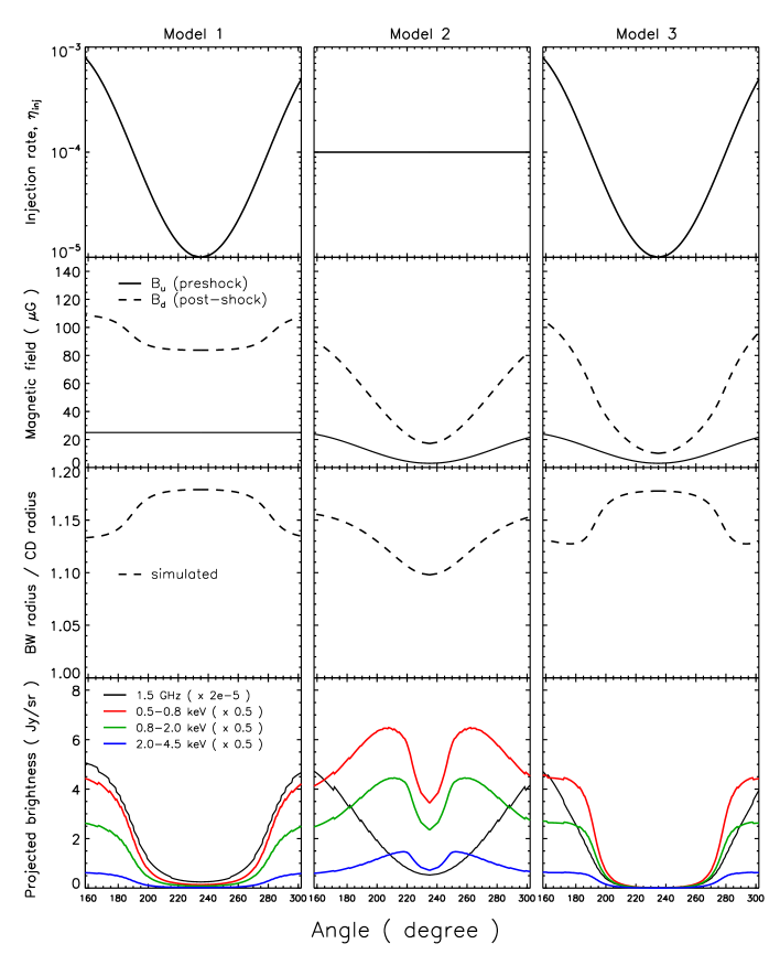
Figure 9: Various models assuming different azimuthal profiles for the injection rate, $\eta_{\mathrm{inj}}$ (top), and far upstream magnetic field, $B_{\mathrm{u}}$ (second, solid lines). Each model predicts azimuthal variations of the ratio of radii between the BW and CD, $R_{\mathrm{BW}}/R_{\mathrm{CD}}$ (third), and synchrotron brightness (projected along the line-of-sight) at different frequencies (bottom).

To understand the influence of these four basic input parameters, we begin first with a heuristic discussion to set the stage for later detailed and more physical models (§5.3.5). In Figure 9, we show three models where we vary the two most important parameters, $\eta_{\mathrm{inj}}$ and $B_{\mathrm{u}}$, with azimuthal angle ($K_{\mathrm{ep}}$ is held constant and $k_{0}$ is set to 1 at all angles). Model 1 (left panels) has $\eta_{\mathrm{inj}}$ varying from $10^{-5}$ to $10^{-3}$, while $B_{\mathrm{u}}$ is held constant at the value $25\;\mu\mathrm{G}$. Model 2 (middle panels) has constant $\eta_{\mathrm{inj}}=10^{-4}$ and $B_{\mathrm{u}}$ varying from $3\;\mu\mathrm{G}$ to $25\;\mu\mathrm{G}$. Model 3 (right panels) is a combination of models 1 and 2 and has $\eta_{\mathrm{inj}}$ varying from $10^{-5}$ to $10^{-3}$ and $B_{\mathrm{u}}$ varying from $3\;\mu\mathrm{G}$ to $25\;\mu\mathrm{G}$.

Note that in all these models, the functional form of the profiles when $\eta_{\mathrm{inj}}$ and $B_{\mathrm{u}}$ vary is rather arbitrary and just used for illustration purposes (for completeness we note that the angular range shown corresponds to the data extraction region in Fig. 7). Moreover, the upstream magnetic field, $B_{\mathrm{u}}$ (second panels, solid lines), is allowed to vary with azimuthal angle because we implicitly assume that it can be significantly amplified by the CR-streaming instability. Our model does not include self-consistently the magnetic field amplification believed to occur at SNR shocks, but is provided with a simple compression. Assuming that the magnetic turbulence is isotropic ahead of the shock, the immediate post-shock magnetic field, $B_{\mathrm{d}}$ (dashed lines), will then be larger than upstream by a factor $r_{B}\equiv B_{\mathrm{d}}/B_{\mathrm{u}}=\sqrt{(1+2\>r_{\mathrm{tot}}^{2})/3}$. This relation is assumed at each azimuthal angle.

We show the predicted profiles of the ratio of radii between the BW and CD (third panels) and synchrotron brightness projected along the line-of-sight in the radio and different X-ray energy bands (bottom panels). We explain later how those brightness profiles were precisely constructed (§5.3.5). Clearly, model 2 does not predict the expected correlation between the ratio of radii and the synchrotron brightness and hence can be rejected immediately. On the other hand, models 1 and 3 lead to the expected correlation: the smaller the BW/CD ratio, the brighter the synchrotron emission. Comparing models 1 or 3 with model 2 allows us to see that only an azimuthal variation of the injection rate leads to the appropriate variation in the ratio of BW to CD radii (third panels). Comparing model 1 with model 3 shows the impact of the magnetic field variations through synchrotron losses on the azimuthal profiles of the X-ray synchrotron emission (bottom panels).

Although models 1 and 3 seem to describe the key observational constraints fairly well, they suffer weaknesses as regards their underlying astrophysical premises. In model 1, it is difficult to justify why the magnetic field should be enhanced in the region of inefficient particle acceleration ($\eta_{\mathrm{inj}}\leq 6\times 10^{-5}$). The model proposes a post-shock magnetic field there of $\sim 80\>\mu\mathrm{G}$, when a value of $10-15\>\mu\mathrm{G}$ would more likely reflect the value of the compressed ambient field. In model 3, it is difficult to understand why the turbulence level would saturate (i.e., $k_{0}=1$) everywhere. Hence, we are led to develop more elaborated models where $k_{0}$ and/or $K_{\mathrm{ep}}$ are allowed to vary with azimuthal angle. A variation of either $k_{0}$ or $K_{\mathrm{ep}}$ will not significantly affect the ratio of BW to CD radii, but will only modify the profiles of the synchrotron emission. In fact, a model with varying $K_{\mathrm{ep}}$ can be already excluded because this quantity changes the radio and X-ray synchrotron intensities in the same way while the observed radio and X-ray profiles (Fig. 7) vary with azimuth in different ways. Varying $k_{0}$ (as we show in §5.3.5) does allow us to modify the relative azimuthal profiles.

5.3.4 Can CR-modified models provide $R_{\mathrm{BW}}/R_{\mathrm{CD}}=1.00$?

Although CR-modified hydrodynamical simulations predict a ratio of radii $R_{\mathrm{BW}}/R_{\mathrm{CD}}$ smaller than standard hydrodynamical simulations, they still predict a lower limit on that ratio that is strictly larger than unity. For instance, Figure 9 (third-right panel) shows that the modeled ratio of radii where the synchrotron emission is strong is $\sim 1.13$. This value was obtained assuming an injection rate of $10^{-3}$ and an ambient magnetic field of 25 $\mu$G. Keeping all the same inputs, but reducing the magnetic field value to 3 $\mu$G, we obtain the lowest possible value of $R_{\mathrm{BW}}/R_{\mathrm{CD}}=1.06$.

On the other hand, the observations of SN 1006 show that the ratio of radii is of order 1.00 in the synchrotron-emitting caps, a value that is not possible to obtain from our CR-modified model under the DSA framework. However, as already mentioned before in our discussions of the small gap between the BW and CD in the region of inefficient acceleration (§5.2), we need to consider projection effects due to hydrodynamical instabilities at the CD which can reduce the gap by $6-10\%$. This does not fully account for the difference with the model and, therefore, we may need to invoke another effect, such as clumping of the ejecta, to fully explain the offset between the observation and models. It is important to note that in both the regions of efficient and inefficient CR acceleration, we require essentially the same numerical factor to bring the modeled ratio of radii (for the appropriate model in each case) into agreement with the observed ratio. In the following, we introduce an ad-hoc rescaling of the ratio of radii by decreasing the modeled values by a constant factor ($\sim 13\%$) at all azimuthal angles. By doing this, we implicitly assume that this factor contains the total contribution of effects that are unrelated to the CR acceleration process. The numerical value used depends, of course, on the particular SN explosion model used. For example, the factor would need to be increased slightly in the case of an exponential ejecta profile (cf., Fig. 8).

5.3.5 Toward a good astrophysical model

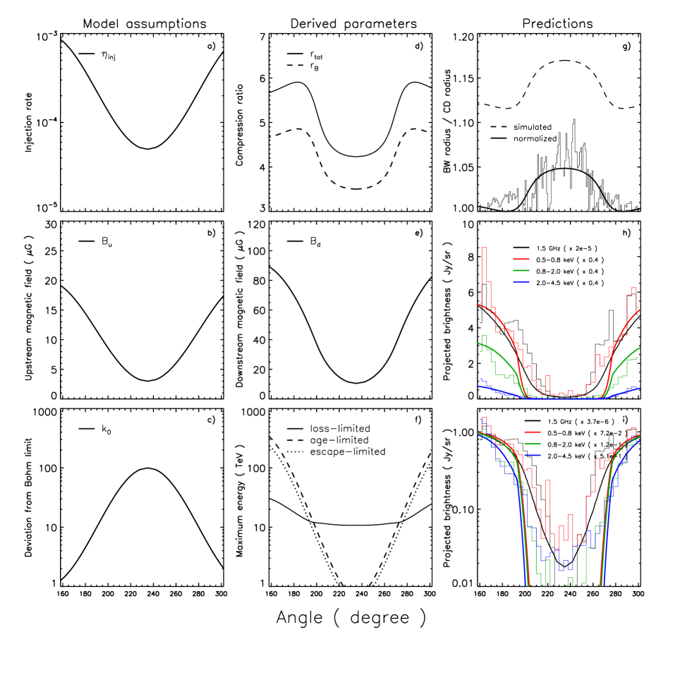
Figure 10: Left column: azimuthal profiles assumed for the injection efficiency, $\eta_{\mathrm{inj}}$ (panel a), far upstream magnetic field, $B_{\mathrm{u}}$ (panel b) and diffusion coefficient normalized to the Bohm-limit value, $k_{0}$ (panel c). Middle column: model profiles of the overall density ($r_{\mathrm{tot}}$) and magnetic field ($r_{B}$) compression ratios (panel d), immediate post-shock value of the magnetic field, $B_{\mathrm{d}}$ (panel e) and maximum energies (panel f). Right column: predicted (thick lines) and observed (thin histograms) azimuthal profiles for the ratio of radii between the BW and CD, $R_{\mathrm{BW}}/R_{\mathrm{CD}}$ (panel g, solid lines) and line-of-sight projected synchrotron brightness at several frequencies (panels h and i).

In Figure 10, we present in more detail what we believe is a reasonable astrophysical model. This model assumes that $\eta_{\mathrm{inj}}$ increases from a value of $5\times 10^{-5}$ to a value of $10^{-3}$ while at the same time $B_{\mathrm{u}}$ increases from a value of $3\;\mu\mathrm{G}$ to a value of $20\;\mu\mathrm{G}$ and $k_{0}$ increases from an arbitrary value of 100 to 1 ($K_{\mathrm{ep}}$ is kept constant at all angles). The azimuthal variations of these parameters is consistent with the picture of DSA where, once the magnetic field fluctuations at the shock exceed the background ISM fluctuations, any low injection rate leads to growth of the turbulent magnetic field in the upstream region, which in turns leads to an increase of the injection rate (Völk et al. 2003). The acceleration efficiency, defined as the fraction of total energy flux crossing the shock that goes into relativistic particles (see §3.3 in Berezhko & Ellison 1999), is $51\%$ in the case with $\eta_{\mathrm{inj}}=10^{-3}$ and $7\%$ in the case with $\eta_{\mathrm{inj}}=5\times 10^{-5}$.

Note that the form of the azimuthal profiles of $\eta_{\mathrm{inj}}$ and $B_{\mathrm{u}}$ is again arbitrary (here a squared-sine variation) and just used for illustration purpose. Our goal is not to find the exact form of the profiles based on an accurate fit of the model predictions to the observations, but rather to describe qualitatively how the acceleration parameters vary along the BW in SN 1006. The extremum values for $\eta_{\mathrm{inj}}$ were chosen so that the predicted variations of the ratio of radii $R_{\mathrm{BW}}/R_{\mathrm{CD}}$ roughly matches the observations. A maximum (minimum) value of $\eta_{\mathrm{inj}}$ between $10^{-4}$ and $10^{-2}$ (resp. $10^{-5}$ and $5\times 10^{-5}$) will not significantly affect our results concerning the profile of $R_{\mathrm{BW}}/R_{\mathrm{CD}}$, but differences will be seen in the absolute intensity in the synchrotron emission. The maximum value of $B_{\mathrm{u}}$ was adjusted so that it yields an immediate postshock value, $B_{\mathrm{d}}\simeq 80\>\mu{\mathrm{G}}$ (panels e), consistent with the value derived from the thickness of the X-ray synchrotron-emitting rims in SN 1006, under the assumption that this thickness is limited by the synchrotron losses of the highest energy electrons (e.g., Ballet 2006). Finally, we adjusted the minimum value of $B_{\mathrm{u}}$ in the faint region so that the predicted and observed radio synchrotron flux are roughly the same; here we show profiles with a value of $B_{\mathrm{u}}=3\>\mu{\mathrm{G}}$, i.e., the typical ISM value.

In Figure 10 (panel g), we show the predicted azimuthal profile of ratio of radii between the BW and CD (dashed lines). The ratio of radii was normalized (solid lines) so that it roughly equals 1.00 in the region of efficient CR acceleration as in the observations. This normalization procedure (which we justified in §5.3.4) works remarkably well. The variations of the ratio of radii reflects nothing but the variations of the overall density compression ratio, $r_{\mathrm{tot}}$ (panel d). For low injection rates ($\eta_{\mathrm{inj}}\leq 6\times 10^{-5}$), the compression ratio comes close to the value obtained in the test-particle case (i.e., $r_{\mathrm{tot}}=4$) and as the injection rate increases, the plasma becomes more compressible with $r_{\mathrm{tot}}\sim 6$. However, once the magnetic field has been considerably amplified ($B_{\mathrm{u}}\geq 10\;\mu\mathrm{G}$), $r_{\mathrm{tot}}$ starts to slightly decrease due to the heating of the gas by the Alfvén waves in the precursor region (see Berezhko & Ellison 1999).

In Figure 10 (panel h), we show the azimuthal profiles of the synchrotron emission in the radio and several X-ray energy bands. To obtain these profiles, we first computed the radial profile of the synchrotron flux (calculated in a given energy band) at each azimuthal angle. Then, we projected the flux along the line-of-sight and finally extracted the projected flux in $30\arcsec$-wide regions behind the BW (assuming a distance of 2 kpc) as we did in the observations of SN 1006 (§4.2). In this procedure, we assumed a spherically symmetric distribution for the emissivity. This is a reasonable assumption as long as we restrict the analysis close to the BW, considering that the bright limbs in SN 1006 are in fact polar caps, i.e., where the emissivity distribution is axisymmetric. Finally, we fixed the radio flux in the synchrotron caps to be the same as in the observations by adjusting the electron-to-proton density ratio at relativistic energies, $K_{\mathrm{ep}}$. This is obtained for a value of $K_{\mathrm{ep}}=7\times 10^{-4}$.

Relaxing the assumption of the Bohm diffusion (i.e., $k_{0}$) at each azimuthal angle significantly modifies the azimuthal profiles of the synchrotron flux in the X-ray band (while the radio profile is unchanged) compared to the model 3 of Figure 9 in which $k_{0}$ was always equal to 1. This is because an increase of $k_{0}$ decreases the maximum energy of electrons, $E_{e,\mathrm{max}}$. Since the synchrotron emission is very sensitive to the position of the high-energy cutoff in the electron distribution (i.e., $E_{e,\mathrm{max}}$), all profiles do not show anymore a plateau in the region of efficient CR acceleration but are now gradually decreasing (panel h). Besides, the synchrotron brightness in the X-ray bands now decreases faster than in the radio (panel i). This is roughly consistent with what is observed in SN 1006. We note that in this model, the maximum energy of both protons and electrons (panel f) decrease rather quickly as we move toward regions of inefficient CR acceleration as opposed to the previous model 3 with $k_{0}=1$ where the maximum energy of electrons remained approximately constant (not shown). Overall, our results from this model are consistent with those of Rothenflug et al. (2004) which were based on a different approach (i.e., measure of the azimuthal variations of the cutoff-frequency all around SN 1006) using XMM-Newton observations.

5.3.6 Other azimuthal profiles for $\eta_{\mathrm{inj}}$, $B_{\mathrm{u}}$ and $k_{0}$

We have found that a simple model in which the injection rate of particles in the acceleration process ($\eta_{\mathrm{inj}}$), amplified magnetic field ($B_{\mathrm{u}}$) and level of turbulence ($k_{0}$) were gradually increasing around the shock front was able to provide predictions in a good agreement with the observations for the azimuthal variations of the ratio of radii and radio and X-ray synchrotron fluxes. The input parameters and their azimuthal variations were chosen based on the physical picture where the injection of particles and amplification of the magnetic turbulence are coupled.

One can imagine however more complicated scenario and hence more complicated input profiles for the acceleration parameters ($\eta_{\mathrm{inj}}$, $B_{\mathrm{u}}$, $k_{0}$). For instance, the coupling between the injection and the turbulence which occurs at the beginning of the acceleration process may end at some point when the amplitude of the magnetic field fluctuations become so high that their further growth is prevented by strong dissipation processes (Völk et al. 2003). The injection, magnetic field and level of turbulence may in fact saturate (over some azimuthal range) as we reach regions of very efficient CR acceleration. Another example of scenario can be imagined if the shock velocity is not uniformly distributed along the shock (as opposed to what we have assumed in our models) due to a asymmetrical explosion. Such a scenario could explain why the bright synchrotron-emitting caps in SN 1006 seem to have larger radii than the faint regions. If so, the injection could be larger in the region of higher velocity while the level of turbulence and magnetic field could potentially saturate there. In general, these new scenarios will not lead to a significant modification of the profile of the ratio of radii. However, we do expect some changes in the azimuthal profiles of the radio and X-ray synchrotron flux. They will generally be flatter in the regions of very efficient CR acceleration.

6 Discussion

6.1 Polar cap morphology

The model in which the injection rate of particles, magnetic field and level of turbulence are all varying as a function of azimuth was successful in reproducing the overall azimuthal variations of the radio and X-ray synchrotron flux observed along the BW of SN 1006 (Fig. 10). In fact, it is actually possible to build a 2-D projected map of the radio and X-ray synchrotron morphology comparable to the radio and X-ray images of SN 1006 (Figs. 1 and 2). This requires us to know the three-dimensional distribution of the emissivity. Here, we consider polar caps as suggested by Rothenflug et al. (2004).

To simplify the calculation, we consider that the radial profiles of the emissivity obtained from the different values of injection, magnetic field and turbulence level have an exponential form characterized by a maximum emissivity at the shock and width $\Delta R$ over which the emissivity decreases (see Appendix A). We also fixed the BW radius, $R_{\mathrm{BW}}$, to be the same at each azimuthal angle where the injection and magnetic field vary, although it slightly depends on the CR acceleration efficiency. These are good approximations.

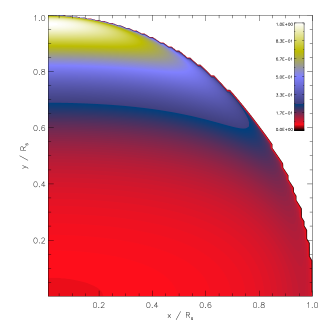
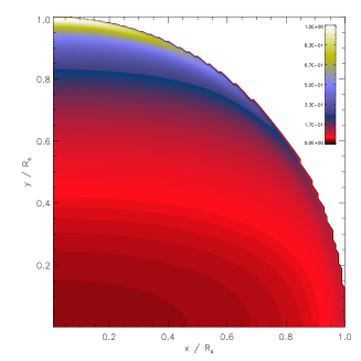
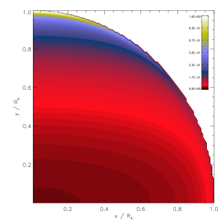
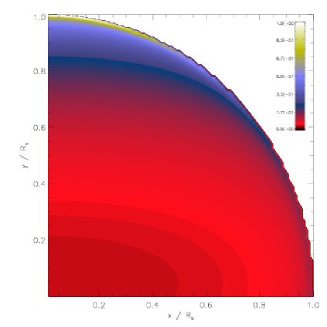
Figure 11: Projected morphology predicted in the case of polar caps (see Appendix A) with $\Delta\tilde{R}=5\times 10^{-2}$ (top-left), $\Delta\tilde{R}=10^{-2}$ (top-right), $\Delta\tilde{R}=5\times 10^{-3}$ (bottom-left), $\Delta\tilde{R}$ linearly varying from $2\times 10^{-3}$ at the pole to $8\times 10^{-3}$ at the equator (bottom-right). The radio and the high-energy X-ray morphology predicted by the model shown in Figure 10 correspond roughly here to the top-right and bottom-right panels, respectively. In all panels, the intensity scaling is square-root.

In the case of the radio synchrotron emission, the width $\Delta R$ does not depend on the azimuthal angle (from the pole to the equator), and we have typically $\Delta\tilde{R}\equiv\Delta R/R_{\mathrm{BW}}=0.01$. The projected radio morphology is shown in Figure 11 (top-right panel). It has a bipolar limb-brightened morphology as is observed in SN 1006.

In the case of the X-ray synchrotron emission, the width $\Delta R$ is expected first to increase (starting from the equator) as particles reach higher energies and the emission builds up, and then to slightly decrease when the effect of radiative losses starts to become important due to the larger post-shock magnetic field as we move toward the pole. Because the brightness is much lower at the equator than at the pole, a reasonable approximation is to consider the width constant with typically $\Delta\tilde{R}=2-5\times 10^{-3}$ (bottom-left panel) or even a slightly increasing width from the pole to the equator (bottom-right panel). A slightly increasing width will not change the overall morphology. It still produces a thin rim whose projected width is decreasing starting from the pole to the equator. In Figure 11, we have assumed that the emissivity contrast at the BW between the pole and the equator is always a factor 100. In fact, because the contrast between the pole and equator is larger in the X-rays than in the radio, we will obtain a similar morphology but with the size of the caps slightly reduced in X-ray. In other words, the X-ray synchrotron emitting rims become geometrically thinner and of smallest azimuthal extent as we go to higher energy. All these effects would be however slightly attenuated if we had included the instrumental effects (particularly the PSF), but overall this is consistent with what is observed in SN 1006.

6.2 CR acceleration in a partially ionized medium

When trying to delineate the BW, we found that the X-ray synchrotron-emitting rims and the diffuse filament of H$\alpha$ emission were coincident over some little azimuthal range, notably for instance at the edge of the eastern cap where the synchrotron emission starts to turn on (see Fig. 1). SN 1006 is one of the rare remnants where this characteristic is clearly observed, although this likely happens in the Tycho SNR too.

In general, H$\alpha$ emission from non-radiative shocks is believed to arise when the blast wave encounters partially ionized gas. This points to the presence of neutral atoms in the ambient medium around SN 1006 (Ghavamian et al. 2002). Theoretical studies have shown that in such medium, the scattering Alfvén waves should be damped, henceforth quenching the acceleration of high energy particles (O’C Drury et al. 1996). In fact, recent theoretical studies suggest that the magnetic field could be turbulently amplified even in such medium (Bykov & Toptygin 2005). The fact that we observe the H$\alpha$ and synchrotron X-rays to be coincident gives support to this statement. Other observations of H$\alpha$ emission coexisting with synchrotron X-rays would be very interesting in that regard.

6.3 Comparison between SN 1006 and Tycho

Like SN 1006, the Tycho SNR is believed to be the remnant of a thermonuclear explosion and, as such, is expected to develop an approximately exponential ejecta density profile and to evolve in a uniform ambient medium. Measurements of the gap between BW and CD have been done in the Tycho SNR using Chandra observations (Warren et al. 2005). We comment on the Tycho results in the light of our results.

Because the thin and bright X-ray synchrotron-emitting rims concentrated at the BW are observed all around Tycho, in contrast to SN 1006, the BW’s location can be easily determined. In addition, because the X-ray emission from the shocked ejecta is dominant in Tycho, in contrast to SN 1006, it is also fairly easy to determine the CD’s location. The observed azimuthally-averaged ratio of radii between the BW and CD was found to be $\sim 1.04$ in Tycho (Warren et al. 2005). After correcting, approximately, for effects due to projection of the highly structured CD, the ratio of radii became $\sim 1.075$. This is still a lot smaller than the (unprojected) ratio of $\sim 1.25$ derived using standard one-dimensional hydrodynamical simulations with no CR acceleration, at the current age of Tycho ($430$ yrs). It was then concluded that efficient CR ion acceleration was occurring around nearly the entire BW of Tycho.

More recently, Cassam-Chenaï et al. (2007) applied a CR-modified self-similar hydrodynamic model to the radio and X-ray observations of the Tycho SNR using the observed ratio of BW to CD radii as an important input constraint. Using reasonable values for the hydrodynamical parameters (ambient medium density, SN explosion energy, ejected mass), DSA parameters (injection efficiency, magnetic field, diffusion coefficient, electron-to-proton ratio at relativistic energies), and the distance, a good description of the observational properties at the blast wave of Tycho was obtained. This detailed study provides a self-consistent/coherent picture of efficient CR ion acceleration.

Regarding SN 1006, we have some good news and some bad (compared to the case of Tycho, where CR-modified models seem to describe the data well). The good news is that there is a significant variation in the ratio of BW to CD radii as a function of azimuthal angle that is correlated with the varying intensity of the X-ray and radio synchrotron emission. Where the gap is large the synchrotron emission is faint (or not detected) and where the gap is small the emission is bright. This is consistent with an azimuthal variation in the effects of CR-modification to the remnant dynamics. The bad news is that in regions of presumably efficient acceleration (i.e., the bright rims), the ratio of BW to CD radii approaches small values, very close to 1. The puzzle is that our CR-modified hydrodynamical models are unable to produce ratio values less than 1.06, while the specific scenarios presented above produce ratio values closer to $1.12$. In order to make progress in our study we decided to introduce an ad-hoc rescaling of the ratio of radii by decreasing the modeled values at all angles by a constant factor of $\sim 12\%$. This procedure works remarkably well and suggests to us that something else, unrelated to the CR acceleration process (such as 3-D projection effects and ejecta clumping), may be responsible for the smaller than expected gap between the BW and CD in SN 1006.

7 Conclusion

Using a combination of radio, optical (H$\alpha$) and X-ray images, we have located the positions of the BW and CD radii along the southeastern sector of SN 1006. We found that with increasing azimuthal angles the ratio of radii between the BW and CD increases from values near unity (within the northeastern synchrotron-emitting cap) to a maximum of about 1.10 before falling again to values near unity (in the southwestern synchrotron-emitting cap). These variations reflect changes in the compressibility of the plasma attributed to variations in the efficiency of the BW at accelerating CR ions and give strong support to the overall picture that SNR shocks produce some fraction of Galactic CRs. However, at the present time we do not have a detailed explanation for the apparent overall smallness of the measured ratios of radii in SN 1006: the minimum value predicted by our CR-modified self-similar dynamical models is 1.06. In this study we simply rescaled the ratio of radii by a constant factor (independent of azimuthal angle) of $\sim 12\%$ with the expectation that some process, other than CR acceleration itself, was responsible for driving the edge of the ejecta closer to the BW all along the rim of SN 1006. The lack of a definitive astrophysical explanation for this discrepancy is a significant factor limiting our ability to understand the CR acceleration process in SN 1006. Further research into the effects of hydrodynamical instabilities at the CD and ejecta clumping (two possible explanations for the small BW/CD ratio) would incidentally provide new insights into the acceleration process.

In addition to the azimuthal variations of the ratio of radii between the BW and CD we also interpreted the variations of the synchrotron flux (at various frequencies) at the BW using CR-modified hydrodynamic models. We assumed different azimuthal profiles for the injection rate of particles in the acceleration process, magnetic field and turbulence level. We found the observations to be consistent with a model in which these quantities are all azimuthally varying, being the largest in the brightest regions. Overall this is consistent with the picture of diffusive shock acceleration. In terms of morphology, we found that our model was generally consistent with the observed properties of SN 1006, i.e., a bright and geometrically-thin synchrotron-emitting rim at the poles and very faint synchrotron emission at the equator and in the interior. In the model, the X-ray synchrotron-emitting rims are geometrically thinner and of smallest azimuthal extent than the radio rims, which is in broad agreement with observations. This is because the most energetic electrons accelerated at the blast wave lose energy efficiently in the amplified post-shock magnetic field. Based on this picture, it would be worth trying to measure the azimuthal variation of the magnetic field strength (from the X-ray rim widths) and thereby gain further insight into the amplification process.

Appendix A Projection along the line-of-sight in the case of polar caps

Let $r$ be the distance to the center $O$ of a sphere of radius $R_{s}$, $\phi$ the azimuthal angle in the $(O\vec{x},O\vec{z})$ plane with $0\leq\phi\leq 2\pi$, and $\theta$ the latitude with $-\pi/2\leq\theta\leq\pi/2$. The projection of a spherical emissivity distribution $\mathcal{E}(r,\theta,\phi)$ onto the plane $(O\vec{x},O\vec{y})$ results in a two-dimensional brightness distribution:

$$\mathcal{B}(x,y)=2\>\int_{0}^{\ell}\mathcal{E}(r,\theta,\phi)\>dz,$$ (A1)

where $\ell^{2}=x_{s}^{2}-x^{2}$, and $0\leq x\leq x_{s}\equiv R_{s}\>\cos\theta$ and $0\leq y\leq R_{s}$. At any point of coordinate $(x,y,z)$, the emissivity is $\mathcal{E}(x,y,z)=\mathcal{E}(r,\theta,\phi)$ where $r^{2}=x^{2}+y^{2}+z^{2}$ and $\theta=\arcsin\left(y/r\right)$ and $\phi=\arccos(x/\sqrt{x^{2}+z^{2}})$. When the emissivity has a symmetry of revolution around the $O\vec{y}$ axis (e.g., polar caps), there is no dependency on $\phi$.

Let us consider a sphere where the emissivity $\mathcal{E}$ is radially decreasing from the maximum $\mathcal{E}_{\mathrm{max}}$ at the surface of the sphere with a characteristic width $\Delta R$. In the case of an exponential decrease and cylindrical symmetry, we have:

$$\mathcal{E}(r,\theta,\phi)=\mathcal{E}_{\mathrm{max}}(\theta)\>\exp\left(\frac{r-R_{s}}{\Delta R(\theta)}\right).$$ (A2)

In the case of polar caps, $\mathcal{E}_{\mathrm{max}}$ will be larger at the poles ($\theta=\pi/2$ and $\theta=-\pi/2$).

In Figure 11, we show the projected morphology obtained with the emissivity spatial distribution given by Eq. (A2) in the range $0\leq\theta\leq\pi/2$ assuming different values and angular dependencies for the width $\Delta\tilde{R}\equiv\Delta R/R_{s}$. In those plots, a squared-sine variation was assumed for ${\log}_{10}\left(\mathcal{E_{\mathrm{max}}}\right)$, having the value $0.0$ at the pole and $-2.0$ at the equator. Decreasing the value at the equator produces similar rims but with a lower azimuthal extent (i.e., smaller polar caps).

References

- Acero et al. (2007) Acero, F., Ballet, J., & Decourchelle, A. 2007, A&A, 475, 883
- Aharonian et al. (2005) Aharonian, F., Akhperjanian, A. G., Aye, K.-M., et al. 2005, A&A, 437, 135
- Aharonian et al. (2007a) Aharonian, F., Akhperjanian, A. G., Bazer-Bachi, A. R., et al. 2007a, A&A, 464, 235
- Aharonian et al. (2007b) Aharonian, F., Akhperjanian, A. G., Bazer-Bachi, A. R., et al. 2007b, ApJ, 661, 236
- Amato & Blasi (2006) Amato, E. & Blasi, P. 2006, MNRAS, 371, 1251
- Badenes et al. (2003) Badenes, C., Bravo, E., Borkowski, K. J., & Domínguez, I. 2003, ApJ, 593, 358
- Badenes et al. (2007) Badenes, C., Hughes, J. P., Bravo, E., & Langer, N. 2007, ApJ, 662, 472
- Ballet (2006) Ballet, J. 2006, Advances in Space Research, 37, 1902
- Bamba et al. (2003) Bamba, A., Yamazaki, R., Ueno, M., & Koyama, K. 2003, ApJ, 589, 827
- Baring (2007) Baring, M. G. 2007, Ap&SS, 307, 297
- Bell (1978) Bell, A. R. 1978, MNRAS, 182, 147
- Berezhko (1996) Berezhko, E. G. 1996, Astroparticle Physics, 5, 367
- Berezhko & Ellison (1999) Berezhko, E. G. & Ellison, D. C. 1999, ApJ, 526, 385
- Berezhko et al. (2002) Berezhko, E. G., Ksenofontov, L. T., & Völk, H. J. 2002, A&A, 395, 943
- Berezhko et al. (2003) Berezhko, E. G., Ksenofontov, L. T., & Völk, H. J. 2003, A&A, 412, L11
- Berezhko & Völk (2006) Berezhko, E. G. & Völk, H. J. 2006, A&A, 451, 981
- Berezhko & Völk (2007) Berezhko, E. G. & Völk, H. J. 2007, ApJ, 661, L175
- Blandford & Ostriker (1978) Blandford, R. D. & Ostriker, J. P. 1978, ApJ, 221, L29
- Blasi (2002) Blasi, P. 2002, Astroparticle Physics, 16, 429
- Blasi et al. (2005) Blasi, P., Gabici, S., & Vannoni, G. 2005, MNRAS, 361, 907
- Blondin & Ellison (2001) Blondin, J. M. & Ellison, D. C. 2001, ApJ, 560, 244
- Bykov & Toptygin (2005) Bykov, A. M. & Toptygin, I. N. 2005, Astronomy Letters, 31, 748
- Cassam-Chenaï et al. (2005) Cassam-Chenaï, G., Decourchelle, A., Ballet, J., & Ellison, D. C. 2005, A&A, 443, 955
- Cassam-Chenaï et al. (2004) Cassam-Chenaï, G., Decourchelle, A., Ballet, J., et al. 2004, A&A, 427, 199
- Cassam-Chenaï et al. (2007) Cassam-Chenaï, G., Hughes, J. P., Ballet, J., & Decourchelle, A. 2007, ApJ, 665, 315
- Chevalier et al. (1992) Chevalier, R. A., Blondin, J. M., & Emmering, R. T. 1992, ApJ, 392, 118
- Decourchelle (2005) Decourchelle, A. 2005, in X-Ray and Radio Connections (eds. L.O. Sjouwerman and K.K Dyer) Published electronically by NRAO, http://www.aoc.nrao.edu/events/xraydio Held 3-6 February 2004 in Santa Fe, New Mexico, USA, (E4.02) 10 pages
- Decourchelle et al. (2000) Decourchelle, A., Ellison, D. C., & Ballet, J. 2000, ApJ, 543, L57
- Dubner et al. (2002) Dubner, G. M., Giacani, E. B., Goss, W. M., Green, A. J., & Nyman, L.-Å. 2002, A&A, 387, 1047
- Dwarkadas (2000) Dwarkadas, V. V. 2000, ApJ, 541, 418
- Dwarkadas & Chevalier (1998) Dwarkadas, V. V. & Chevalier, R. A. 1998, ApJ, 497, 807
- Ellison et al. (1995) Ellison, D. C., Baring, M. G., & Jones, F. C. 1995, ApJ, 453, 873
- Ellison et al. (2000) Ellison, D. C., Berezhko, E. G., & Baring, M. G. 2000, ApJ, 540, 292
- Ellison & Cassam-Chenaï (2005) Ellison, D. C. & Cassam-Chenaï, G. 2005, ApJ, 632, 920
- Ellison et al. (2004) Ellison, D. C., Decourchelle, A., & Ballet, J. 2004, A&A, 413, 189
- Ferrière (2001) Ferrière, K. M. 2001, Reviews of Modern Physics, 73, 1031
- Ghavamian et al. (2002) Ghavamian, P., Winkler, P. F., Raymond, J. C., & Long, K. S. 2002, ApJ, 572, 888
- Hamilton et al. (2007) Hamilton, A. J. S., Fesen, R. A., & Blair, W. P. 2007, MNRAS, 381, 771
- Heng & McCray (2007) Heng, K. & McCray, R. 2007, ApJ, 654, 923
- Hoppe et al. (2007) Hoppe, S., Lemoine-Goumard, M., & for the H. E. S. S. Collaboration. 2007, ArXiv e-prints, 709
- Jones & Ellison (1991) Jones, F. C. & Ellison, D. C. 1991, Space Science Reviews, 58, 259
- Kane et al. (2000) Kane, J., Arnett, D., Remington, B. A., et al. 2000, ApJ, 528, 989
- Katz & Waxman (2008) Katz, B. & Waxman, E. 2008, Journal of Cosmology and Astro-Particle Physics, 1, 18
- Korreck et al. (2004) Korreck, K. E., Raymond, J. C., Zurbuchen, T. H., & Ghavamian, P. 2004, ApJ, 615, 280
- Ksenofontov et al. (2005) Ksenofontov, L. T., Berezhko, E. G., & Völk, H. J. 2005, A&A, 443, 973
- Leonard et al. (2005) Leonard, D. C., Li, W., Filippenko, A. V., Foley, R. J., & Chornock, R. 2005, ApJ, 632, 450
- Long et al. (2003) Long, K. S., Reynolds, S. P., Raymond, J. C., et al. 2003, ApJ, 586, 1162
- Malkov & O’C Drury (2001) Malkov, M. A. & O’C Drury, L. 2001, Reports of Progress in Physics, 64, 429
- Matzner & McKee (1999) Matzner, C. D. & McKee, C. F. 1999, ApJ, 510, 379
- Moffett et al. (2004) Moffett, D., Caldwell, C., Reynoso, E., & Hughes, J. 2004, in IAU Symposium, Vol. 218, Young Neutron Stars and Their Environments, ed. F. Camilo & B. M. Gaensler, 69–+
- Moffett et al. (1993) Moffett, D. A., Goss, W. M., & Reynolds, S. P. 1993, AJ, 106, 1566
- Nomoto et al. (1984) Nomoto, K., Thielemann, F.-K., & Yokoi, K. 1984, ApJ, 286, 644
- O’C Drury et al. (1996) O’C Drury, L., Duffy, P., & Kirk, J. G. 1996, A&A, 309, 1002
- Orlando et al. (2007) Orlando, S., Bocchino, F., Reale, F., Peres, G., & Petruk, O. 2007, A&A, 470, 927
- Parizot et al. (2006) Parizot, E., Marcowith, A., Ballet, J., & Gallant, Y. A. 2006, A&A, 453, 387
- Plaga (2008) Plaga, R. 2008, New Astronomy, 13, 73
- Porter et al. (2006) Porter, T. A., Moskalenko, I. V., & Strong, A. W. 2006, ApJ, 648, L29
- Raymond et al. (1995) Raymond, J. C., Blair, W. P., & Long, K. S. 1995, ApJ, 454, L31+
- Raymond et al. (2007) Raymond, J. C., Korreck, K. E., Sedlacek, Q. C., et al. 2007, ApJ, 659, 1257
- Reynolds (1998) Reynolds, S. P. 1998, ApJ, 493, 375
- Reynolds & Gilmore (1986) Reynolds, S. P. & Gilmore, D. M. 1986, AJ, 92, 1138
- Reynolds & Gilmore (1993) Reynolds, S. P. & Gilmore, D. M. 1993, AJ, 106, 272
- Reynoso et al. (2008) Reynoso, E. M., Castelletti, G. M., Moffett, D. A., & Hughes, J. P. 2008, RMxAAC, 27
- Rothenflug et al. (2004) Rothenflug, R., Ballet, J., Dubner, G., et al. 2004, A&A, 425, 121
- Sollerman et al. (2003) Sollerman, J., Ghavamian, P., Lundqvist, P., & Smith, R. C. 2003, A&A, 407, 249
- Uchiyama et al. (2007) Uchiyama, Y., Aharonian, F. A., Tanaka, T., Takahashi, T., & Maeda, Y. 2007, Nature, 449, 576
- Vink et al. (2003) Vink, J., Laming, J. M., Gu, M. F., Rasmussen, A., & Kaastra, J. S. 2003, ApJ, 587, L31
- Völk et al. (2003) Völk, H. J., Berezhko, E. G., & Ksenofontov, L. T. 2003, A&A, 409, 563
- Wang & Chevalier (2001) Wang, C.-Y. & Chevalier, R. A. 2001, ApJ, 549, 1119
- Warren et al. (2005) Warren, J. S., Hughes, J. P., Badenes, C., et al. 2005, ApJ, 634, 376
- Winkler et al. (2003) Winkler, P. F., Gupta, G., & Long, K. S. 2003, ApJ, 585, 324
- Winkler & Long (1997) Winkler, P. F. & Long, K. S. 1997, ApJ, 491, 829
- Winkler et al. (2005) Winkler, P. F., Long, K. S., Hamilton, A. J. S., & Fesen, R. A. 2005, ApJ, 624, 189
- Yamaguchi et al. (2007) Yamaguchi, H., Koyama, K., Katsuda, S., et al. 2007, ArXiv e-prints, 706