Bound States in Time-Dependent Quantum Transport: Oscillations and Memory Effects in Current and Density

Abstract

The presence of bound states in a nanoscale electronic system attached to two biased, macroscopic electrodes is shown to give rise to persistent, non-decaying, localized current oscillations which can be much larger than the steady part of the current. The amplitude of these oscillations depends on the entire history of the applied potential. The bound-state contribution to the static density is history-dependent as well. Moreover, the time-dependent formulation leads to a natural definition of the bound-state occupations out of equilibrium.

In recent years it has become possible to measure the current through single molecules attached to two macroscopic electrodes M.A. Reed et al. (1997); A.I. Yanson et al. (1998). This is hoped to be a first step towards the vision of “Molecular Electronics” where single molecules become the basic units (transistors, etc.) of highly miniaturized electronic devices.

To address electronic transport on such a small scale theoretically, one needs a full quantum description of the electronic dynamics. Non-equilibrium Green’s functions (NEGF) provide a natural framework to study quantum transport properties of nanoscale devices coupled to leads. When a bias is applied, the electrodes remain in local equilibrium while the current is driven by the different chemical potentials in the left and right lead. In model systems the leads are assumed to be non-interacting and the current is computed from the Meir-Wingreen formulaMeir and N.S. Wingreen (1992) using approximate many-body self-energies $\Sigma_{\rm MB}$. For weakly correlated models $\Sigma_{\rm MB}\sim 0$ and the Meir-Wingreen formula reduces to the Landauer-Büttiker formulaLandauer (1957); Büttiker (1986), as it should.

If one wants to account for the full atomistic structure of the system, the NEGF formalism is usually combined with static density functional theory (DFT) and the current is computed from a Landauer-type equation N.D. Lang (1995); Hirose and Tsukada (1995); J.M. Seminario et al. (1998); Taylor et al. (2001); Palacios et al. (2001); Xue et al. (2002); Brandbyge et al. (2002); Evers et al. (2004); Faleev et al. (2005). This approach enjoys increasing popularity, in particular for the description of transport experiments on single molecules M.A. Reed et al. (1997). From a fundamental point of view, however, the use of static DFT - which is an equilibrium theory - is not justified to describe non-equilibrium situations. For a critical review of this methodology, the reader is referred to Ref. Koentopp et al., 2008.

By construction, the NEGF+DFT approach inherits the main assumption of the Landauer formalism that for a system driven out of equilibrium by a dc bias, a steady current will eventually develop. In other words, the dynamical formation of a steady state does not follow from the formalism but rather constitutes an assumption. The question of how the system reaches the steady state has been addressed theoretically in Refs. Stefanucci and C.-O. Almbladh, 2004a, b where it was shown that the total current (and the density) reaches a steady value if the local density of states is a smooth function of energy in the device region. In the same work it was also shown that for non-interacting electrons the steady current is independent both of the initial conditions and of the history of the bias, i.e., all memory effects are washed out.

The situation is different, however, if there exist two or more localized bound states (BS) in the device region, i.e., if the local density of states has sharp peaks at certain energies. This case has been investigated in Ref. Dhar and Sen, 2006 and further been elaborated in Ref. Stefanucci, 2007 where it was shown analytically that a non-interacting system with bound states exposed to a dc bias does not evolve to a steady state. Instead, a steady component of the current is superimposed by undamped harmonic current oscillations: Assuming that the one-particle Hamiltonian $\mbox{\boldmath$H$}(t)$ globally converges to a time-independent Hamiltonian $\mbox{\boldmath$H$}^{\infty}$ when $t\rightarrow\infty$, the total current through a plane $\Pi$ perpendicular to the transport geometry has the form

$$\lim_{t\rightarrow\infty}I_{\Pi}(t)=I_{\Pi}^{(S)}+I_{\Pi}^{(D)}(t)\;,$$ (1)

where the static contribution $I_{\Pi}^{(S)}$ is given by the Landauer formula. The dynamical part, $I_{\Pi}^{(D)}(t)$, reads (atomic units are used throughout)

$$I_{\Pi}^{(D)}(t)=2\sum_{b,b^{\prime}}{f_{b,b^{\prime}}\Lambda_{b,b^{\prime}}^{\Pi}\sin[(\epsilon_{b}^{\infty}-\epsilon_{b^{\prime}}^{\infty})t]},$$ (2)

where the summation is over all BS of the final Hamiltonian $\mbox{\boldmath$H$}^{\infty}$ and the oscillation frequencies are given by the BS eigenenergy differences. The quantities ${\Lambda}^{\Pi}_{b,b^{\prime}}$ and $f_{b,b^{\prime}}$ are defined according to

$$\Lambda_{b,b^{\prime}}^{\Pi}=\int_{\Pi}{\rm d}\sigma{\rm d}\sigma^{\prime}\psi^{\infty}_{b^{\prime}}(\mbox{\boldmath$r$}^{\prime})\Sigma(\mbox{\boldmath$r$}^{\prime},\mbox{\boldmath$r$};\epsilon^{\infty}_{b^{\prime}})\psi^{\infty}_{b}(\mbox{\boldmath$r$}),$$ (3)

and

$$f_{b,b^{\prime}}=\langle\psi^{\prime}_{b}|f(\mbox{\boldmath$H$}^{0})|\psi^{\prime}_{b^{\prime}}\rangle\;.$$ (4)

In Eq. (3) the double surface integral is over the plane $\Pi$, $\Sigma$ is the embedding self-energy and $\psi^{\infty}_{b}(\mbox{\boldmath$r$})$ are BS eigenfunctions. The operator $f(\mbox{\boldmath$H$}^{0})$ in Eq. (4) is the Fermi function calculated at the equilibrium Hamiltonian $\mbox{\boldmath$H$}^{0}$ while the state $|\psi^{\prime}_{b}\rangle$ is related to $|\psi_{b}^{\infty}\rangle$ by a unitary transformation: $|\psi^{\prime}_{b}\rangle=\mbox{\boldmath$M$}|\psi_{b}^{\infty}\rangle$. The “memory operator” $M$ depends on the history of the TD perturbation. Therefore the coefficients $f_{b,b^{\prime}}$ are matrix elements of $f(\mbox{\boldmath$H$}^{0})$ between history-dependent localized functions.

In the present work we study these time-dependent (TD) phenomena for a number of numerical examples using a recently proposed algorithm for TD transport Kurth et al. (2005). We show numerically that the amplitude of the current oscillations may be very large compared to the steady component of the current. In addition, the memory dependence of the current oscillations will be explicitly demonstrated. Furthermore, we address an important aspect which, in the NEGF+DFT approach, has remained an open problem, namely how to take BS into account in the calculation of the density Xue et al. (2002); S.-H. Ke et al. (2004). Recently, a somewhat empirical scheme was suggested on how to occupy BS with energies in the bias window Li et al. (2007). Here we will show how the BS occupations naturally result from the time evolution of the underlying KS system. Moreover, for non-interacting electrons we provide numerical evidence that these occupations (and therefore the density in the device region) show a history dependence as well.

In the long-time limit, the dynamical contribution to the density is given by

$$n^{(D)}(\mbox{\boldmath$r$},t)=\sum_{b,b^{\prime}}{f_{b,b^{\prime}}\cos[(\epsilon_{b}^{\infty}-\epsilon_{b^{\prime}}^{\infty})t]\psi_{b}^{\infty}(\mbox{\boldmath$r$})\psi_{b^{\prime}}^{\infty}(\mbox{\boldmath$r$})},$$ (5)

where the amplitudes $f_{b,b^{\prime}}$ are again given by Eq. (4). We observe that while the diagonal term, $b=b^{\prime}$, does not contribute to the current of Eq. (2), it does contribute to the density of Eq. (5) with a history-dependent coefficient $f_{b,b}$. This means that even if we average out the density oscillations, history dependent effects will show up in the density at the device region. This is a central result of our analysis.

In order to shed more light on the actual dependence of the coefficients $f_{b,b^{\prime}}$ on the history of the TD perturbation we study model systems of non-interacting electrons using a recently proposed algorithm Kurth et al. (2005) suitable to describe TD transport through open systems. The central feature of this algorithm is that it allows for the numerically exact solution of the TD Schrödinger equation in the central device region in the presence of the semi-infinite electrodes.

We consider one-dimensional systems described by the TD Hamiltonian

$$H(x,t)=-\frac{1}{2}\frac{{\rm d}^{2}}{{\rm d}x^{2}}+U_{0}(x)+U(x,t)\;.$$ (6)

For times $t<0$ the system is in its ground state described by the Hamiltonian $H^{0}(x)=-\frac{\nabla^{2}}{2}+U_{0}(x)$. At $t=0$ the system is driven out of equilibrium by applying a TD field $U(x,t)$. We choose the TD perturbation in such a way that for ${t\rightarrow\infty}$ the Hamiltonian globally converges to an asymptotic Hamiltonian, $H^{\infty}$.

The TD perturbation can be split into three sub-regions depending on where in the system it is imposed: $U_{\alpha}$, $\alpha=L,R$, represents the applied bias in the left ($L$) and right ($R$) leads and is independent of the position within the lead. In the central region, the TD perturbation (which we call a gate voltage $V_{g}(x,t)$) may depend both on position $x$ and time $t$. Thus, the total TD perturbation can be written as

$$U(x,t)=\left\{\begin{array}[]{cc}U_{L}(t)&-\infty<x<x_{L}\\ V_{g}(x,t)&x_{L}<x<x_{R}\\ U_{R}(t)&x_{R}<x<\infty\end{array}\right..$$ (7)

In the numerical simulations described below, the explicit propagation window ranges from $x_{L}=-1.2$ a.u. to $x_{R}=1.2$ a.u.. We choose a lattice spacing $\Delta x=0.012$ a.u. and use a simple three-point discretization for the kinetic energy. The initial potential is $U_{0}(x)=0$ for any point $x$ in the left or right lead. Therefore, the occupied part of the continuous spectrum ranges from momenta $k=-k_{\rm F}=-\sqrt{2\varepsilon_{\rm F}}$ to $k=k_{\rm F}$ which is discretized with 400 $k$-points ($\varepsilon_{\rm F}$ being the Fermi energy). The (non-interacting) many-body state is propagated from $t=0$ to $t=1400$ a.u. using a time step $\Delta t=0.05$ a.u..

In the first model the initial state is a Slater determinant of plane waves with energies less than $\varepsilon_{\rm F}=0.1$ a.u.. At $t=0$ we suddenly switch on a bias $U_{L}=0.15$ a.u. in the left lead and as a result a current flows which after some transient time reaches a steady value of about $0.027$ a.u.. After the steady state is attained, at time $T=100$ a.u., we switch on a gate potential

$$V_{g}(x,t)=-\frac{(t-T)}{T_{g}}v_{g}$$ (8)

for $T<t<T+T_{g}$ with a switching time $T_{g}=20$ a.u. and the final depth of the potential well $v_{g}=1.3$ a.u.. For times $t\geq T+T_{g}$ this gate potential remains unchanged at $V_{g}(x,t)=-v_{g}$ and supports two BS at $\varepsilon_{1}^{\infty}=-0.933$ a.u. and $\varepsilon_{2}^{\infty}=-0.063$ a.u..

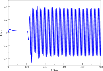
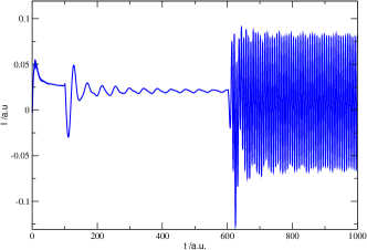
Figure 1: Time evolution of the current at $x=0$. At $t=0$ a.u., a bias $U_{L}=0.15$ a.u. is suddenly switched on and the system evolves to a steady state. Upper panel: at $T=100$ a.u., a gate potential is turned on ($v_{g}=1.3$ a.u. and $T_{g}=20$ a.u.) which creates two BS and results in large amplitude oscillations of the current. Lower panel: at $T=100$ a.u., a first gate potential ($v_{g}=0.2$ a.u. and $T_{g}=0$) is turned on which creates a single BS. Waiting for the transients to decay, a second gate voltage ($v_{g}=1.1$ a.u. and $T_{g}=20$ a.u.) is then applied which leads to the formation of a second BS and therefore to persistent current oscillations. Although $\mbox{\boldmath$H$}^{\infty}$ is identical in both cases, the amplitude of the current oscillation is significantly smaller in the second case, illustrating its dependence on the history of the system.

The resulting TD current in the center of the device region is shown in the upper panel of Fig. 1. The development of a steady-state current for $T<100$ a.u. can clearly be recognized. After the BS are created ($t>T+T_{g}$) the current starts to oscillate as expected. The amplitude of the current oscillation is of the order of 0.35 a.u., i.e., more than an order magnitude larger than the steady-state current. By Fourier transforming the TD current one can identify various transitions which contribute to the oscillating behavior. In the long-time limit, only the transition between BS survives. In the transient regime, however, one finds additional, power-law decaying ($1/t$) transitions from BS to the right continuum at $\varepsilon_{\rm F}$ as well as to the left continuum at $\varepsilon_{\rm F}+U_{L}$ Stefanucci et al. (2008).

The history dependence of the current oscillations can be seen by comparing the current in the upper and lower panels of Fig. 1. Both currents were computed by starting from the same initial state and applying the same bias at $t=0$. In the lower panel we create the same, final potential as in the upper panel, but in two steps. At $T=100$ a.u. we suddenly switch on a first gate potential with depth $v_{g}=0.2$ a.u. which creates one BS. Waiting for the slow decay of the resulting bound-continuum transition we then apply an additional gate potential of depth $v_{g}=1.1$ a.u. (hence the total depth is 1.3 a.u.) with a switching time $T_{g}=20$ a.u.. Again we recognize the persistent current oscillations due to the bound-bound transitions. Although the amplitude (about 0.07 a.u.) is still large compared to the steady-state current, it is about a factor of four smaller than the amplitude in the previous case.

Memory effects not only appear in the amplitude of the current oscillations but also in the BS contribution to the density $n^{(D)}$ (Eq. (5)) through the history dependence of the coefficients $f_{b,b^{\prime}}$ of Eq. (4). In the long-time limit, BS lead to oscillations in $n^{(D)}$ (which are connected to the current oscillations through the continuity equation) and also contribute to the steady part of $n^{(D)}$. This contribution is given by the diagonal part ($b=b^{\prime}$) of the double sum in Eq. (5) which implies that $f_{b,b}$ may be interpreted as occupation numbers of the BS in the long-time limit. In this way, the TD description provides a natural way to include BS in a transport calculation. In the framework of the Landauer formalism this can only be achieved in a somewhat artificial way Li et al. (2007).

We emphasize that also the diagonal occupations $f_{b,b}$ depend on the history through the memory operator $M$. Here we address the importance of this memory dependence which is rather crucial in the NEGF+DFT approach since BS below the bias window are entirely populated, i.e., $f_{b,b}=1$. We have computed the time averaged density $n_{\rm av}(x)$ over an oscillation period for a system with two bound states in the final Hamiltonian. The system is the one which leads to the current shown in the the upper panel of Fig. 1 except that the gate potential is turned on with different switching times $T_{g}$. In Fig. 2 we show $n_{\rm av}(x)$ for three different $T_{g}$ and, as one can see, $n_{\rm av}$ differs quite substantially. This difference has to be attributed to BS since for the contribution of the scattering states all memory is washed out Stefanucci and C.-O. Almbladh (2004b). Of course, the relative importance of the BS contribution to $n_{\rm av}(x)$ will decrease if $\varepsilon_{\rm F}$ (and therefore the contribution of the continuum states) increases.

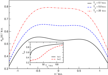
Figure 2: Memory effects for the static part of the density in the long-time limit in the presence of BS. The densities shown here correspond to systems which are identical to the one studied in the upper panel of Fig. 1 except that they are computed for three different switching times of the gate potential of Eq. (8): $T_{g}=0.1$ a.u. (solid, black), $T_{g}=5.0$ a.u. (dashed, blue), and $T_{g}=20$ a.u. (dash-dotted, red). The inset shows the occupation numbers $f_{b,b}$ (Eq. (4)) of the two bound states as function of switching time. The state with lower energy eigenvalue ($b=1$) has higher occupation than the one with higher energy. For short switching times the occupation is significantly smaller than one, while for adiabatic (slow) switching both occupation numbers approach one.

By subtracting the continuum contribution from $n_{\rm av}$ and fitting the explicit function $n^{(D)}$ with the numerical curve (where the only fitting parameters are the coefficients $f_{b,b}$ for $b=1,2$) we have been able to calculate the BS occupations $f_{b,b}$. Remarkably we have found that $f_{b,b}$ exhibits rather large deviations from unity, particularly for small switching times (see inset of Fig. 2). As one would intuitively expect, the occupation of the state with lower energy ($b=1$) is larger than for the state with higher energy. In the adiabatic limit of very slow switching ($T_{g}\to\infty$), both occupation numbers approach unity which is expected since both states are energetically below $\varepsilon_{\rm F}$. The occupation numbers also offer an intuitive qualitative picture of the size of the current and density oscillations: for relatively short switching times ($T_{g}\leq 50$ a.u.) the occupation numbers deviate substantially from one. Therefore the transition probability between the bound states is relatively large and so are the oscillations in current and density. On the other hand, for large switching times both bound states are almost “fully” occupied and the probability of a transition between them is small, leading to small amplitudes in the dynamical density.

We have noticed that in the limit of slow switching the (transient) transitions between bound states and continuum can have a rather large amplitude shortly after the gate potential is applied, even larger than the (persistent) transition between the bound states. As a consequence of the very slow decay of the bound-continuum transitions, one has to propagate for a rather long time before the dynamical part of the density takes on the form of Eq. (5).

In summary we have demonstrated that 1) the persistent current oscillations in the presence of BS can be much larger than the steady-state current 2) the amplitude of the current oscillations can have a strong dependence on the history of the system 3) a similar history dependence is found both for the static and dynamic contribution of the BS to the density and 4) the occupation of the BS is well defined in a TD description of quantum transport.

In the calculations of the present work we assume the electrons to be non-interacting. However, the central conclusions (bound-state oscillations in current and density, memory effects in both quantities) remain valid for any effective single-particle theory such as, e.g., TD Hartree-Fock or TDDFT. In this case, the existence of BS eigensolution of $\mbox{\boldmath$H$}^{\infty}$ is in general not consistent with the assumption of a steady state and the use of the popular NEGF+DFT formalism becomes questionable.

We gratefully acknowledge financial support by the Deutsche Forschungsgemeinschaft through the SFB 658, and the EU Network of Excellence NANOQUANTA (NMP4-CT-2004-500198).

References

- M.A. Reed et al. (1997) M.A. Reed, C. Zhou, C.J. Muller, T.P. Burgin, and J.M. Tour, Science 278, 252 (1997).
- A.I. Yanson et al. (1998) A.I. Yanson, G. Rubio Bollinger, H.E. van den Brom, N.Agraït, and J.M. van Ruitenbeek, Nature 395, 783 (1998).
- Meir and N.S. Wingreen (1992) Y. Meir and N.S. Wingreen, Phys. Rev. Lett. 68, 2512 (1992).
- Landauer (1957) R. Landauer, IBM J. Res. Develop. 1, 233 (1957).
- Büttiker (1986) M. Büttiker, Phys. Rev. Lett. 57, 1761 (1986).
- N.D. Lang (1995) N.D. Lang, Phys. Rev. B 52, 5335 (1995).
- Hirose and Tsukada (1995) K. Hirose and M. Tsukada, Phys. Rev. B 51, 5278 (1995).
- J.M. Seminario et al. (1998) J.M. Seminario, A.G. Zacarias, and J.M. Tour, J. Am. Chem. Soc. 120, 3970 (1998).
- Taylor et al. (2001) J. Taylor, H. Guo, and J. Wang, Phys. Rev. B 63, 245407 (2001).
- Palacios et al. (2001) J. J. Palacios, A. J. Pérez-Jiménez, E. Louis, and J. Vergés, Phys. Rev. B 64, 115411 (2001).
- Xue et al. (2002) Y. Xue, S. Datta, and M.A. Ratner, Chem. Phys. 281, 151 (2002).
- Brandbyge et al. (2002) M. Brandbyge, J.-L. Mozos, P. Ordejón, J. Taylor, and K. Stokbro, Phys. Rev. B 65, 165401 (2002).
- Evers et al. (2004) F. Evers, F. Weigend, and M. Koentopp, Phys. Rev. B 69, 235411 (2004).
- Faleev et al. (2005) S. V. Faleev, F. Leonard, D. A. Stewart, and M. van Schilfgaarde, Phys. Rev. B 71, 195422 (2005).
- Koentopp et al. (2008) M. Koentopp, C. Chang, K. Burke, and R. Car, J. Phys. Condens. Matter 20, 083203 (2008).
- Stefanucci and C.-O. Almbladh (2004a) G. Stefanucci and C.-O. Almbladh, Europhys. Lett. 67, 14 (2004a).
- Stefanucci and C.-O. Almbladh (2004b) G. Stefanucci and C.-O. Almbladh, Phys. Rev. B 69, 195318 (2004b).
- Dhar and Sen (2006) A. Dhar and D. Sen, Phys. Rev. B 73, 085119 (2006).
- Stefanucci (2007) G. Stefanucci, Phys. Rev. B 75, 195115 (2007).
- Kurth et al. (2005) S. Kurth, G. Stefanucci, C.-O. Almbladh, A. Rubio, and E.K.U. Gross, Phys. Rev. B 72, 035308 (2005).
- S.-H. Ke et al. (2004) S.-H. Ke, H. Baranger, and W. Yang, Phys. Rev. B 70, 085410 (2004).
- Li et al. (2007) R. Li, J. Zhang, S. Hou, Z. Qian, Z. Shen, X. Zhao, and Z. Xue, Chem. Phys. 336, 127 (2007).
- Stefanucci et al. (2008) G. Stefanucci, S. Kurth, A. Rubio, and E.K.U. Gross, Phys. Rev. B 77, 075339 (2008).