Spectrum of the Laplacian in a narrow curved strip with combined Dirichlet and Neumann boundary conditions

Abstract

We consider the Laplacian in a domain squeezed between two parallel curves in the plane, subject to Dirichlet boundary conditions on one of the curves and Neumann boundary conditions on the other. We derive two-term asymptotics for eigenvalues in the limit when the distance between the curves tends to zero. The asymptotics are uniform and local in the sense that the coefficients depend only on the extremal points where the ratio of the curvature radii of the Neumann boundary to the Dirichlet one is the biggest. We also show that the asymptotics can be obtained from a form of norm-resolvent convergence which takes into account the width-dependence of the domain of definition of the operators involved.

• 35P15; 49R50; 58J50; 81Q15.

• Laplacian in tubes; Dirichlet and Neumann boundary conditions; dimension reduction; norm-resolvent convergence; binding effect of curvature; waveguides.

• ESAIM: Control, Optimisation and Calculus of Variations
  http://www.esaim-cocv.org

1 Introduction

Given an open interval $I\subseteq\mathbb{R}$ (bounded or unbounded), let $\gamma\in C^{2}(\overline{I};\mathbb{R}^{2})$ be a unit-speed planar curve. The derivative $\dot{\gamma}\equiv(\dot{\gamma}^{1},\dot{\gamma}^{2})$ and $n:=(-\dot{\gamma}^{2},\dot{\gamma}^{1})$ define unit tangent and normal vector fields along $\gamma$, respectively. The curvature is defined through the Frenet-Serret formulae by $\kappa:=\det(\dot{\gamma},\ddot{\gamma})$; it is a bounded and uniformly continuous function on $I$.

For any positive $\varepsilon$, we introduce a mapping $\mathcal{L}_{\varepsilon}$ from $\overline{I}\times[0,1]$ to $\mathbb{R}^{2}$ by

$$\mathcal{L}_{\varepsilon}(s,t):=\gamma(s)+\varepsilon\,t\,n(s)\,.$$ (1.1)

Assuming that $\mathcal{L}_{\varepsilon}$ is injective and that $\varepsilon$ is so small that the supremum norm of $\kappa$ is less than $\varepsilon^{-1}$, $\mathcal{L}_{\varepsilon}$ induces a diffeomorphism and the image

$$\Omega_{\varepsilon}:=\mathcal{L}_{\varepsilon}\big{(}I\times(0,1)\big{)}$$ (1.2)

has a geometrical meaning of an open non-self-intersecting strip, contained between the parallel curves $\gamma(I)$ and $\gamma_{\varepsilon}(I):=\mathcal{L}_{\varepsilon}(I\times\{1\})$, and, if $\partial I$ is not empty, the straight lines $\mathcal{L}_{\varepsilon}\big{(}\{\inf I\}\times(0,1)\big{)}$ and $\mathcal{L}_{\varepsilon}\big{(}\{\sup I\}\times(0,1)\big{)}$. The geometry is set in such a way that $\kappa>0$ implies that the parallel curve $\gamma_{\varepsilon}$ is “locally shorter” than $\gamma$, and vice versa, cf Figure 1.

Let $-\Delta_{DN}^{\Omega_{\varepsilon}}$ be the Laplacian in $L^{2}(\Omega_{\varepsilon})$ with Dirichlet and Neumann boundary conditions on $\gamma$ and $\gamma_{\varepsilon}$, respectively. If $\partial I$ is not empty, we impose Dirichlet boundary conditions on the remaining parts of $\partial\Omega_{\varepsilon}$.

For any self-adjoint operator $H$ which is bounded from below, we denote by $\{\lambda_{j}(H)\}_{j=1}^{\infty}$ the non-decreasing sequence of numbers corresponding to the spectral problem of $H$ according to the Rayleigh-Ritz variational formula [4, Sec. 4.5]. Each $\lambda_{j}(H)$ represents either a (discrete) eigenvalue (repeated according to multiplicity) below the essential spectrum or the threshold of the essential spectrum of $H$. All the eigenvalues below the essential spectrum may be characterized by this variational/minimax principle.

Under the above assumptions, our main result reads as follows:

Theorem 1.1.

For all $j\geq 1$,

$$\lambda_{j}(-\Delta_{DN}^{\Omega_{\varepsilon}})\ =\ \left(\frac{\pi}{2\varepsilon}\right)^{2}+\frac{\inf\kappa}{\varepsilon}+o(\varepsilon^{-1})\qquad\mbox{as}\qquad\varepsilon\to 0\,.$$ (1.3)

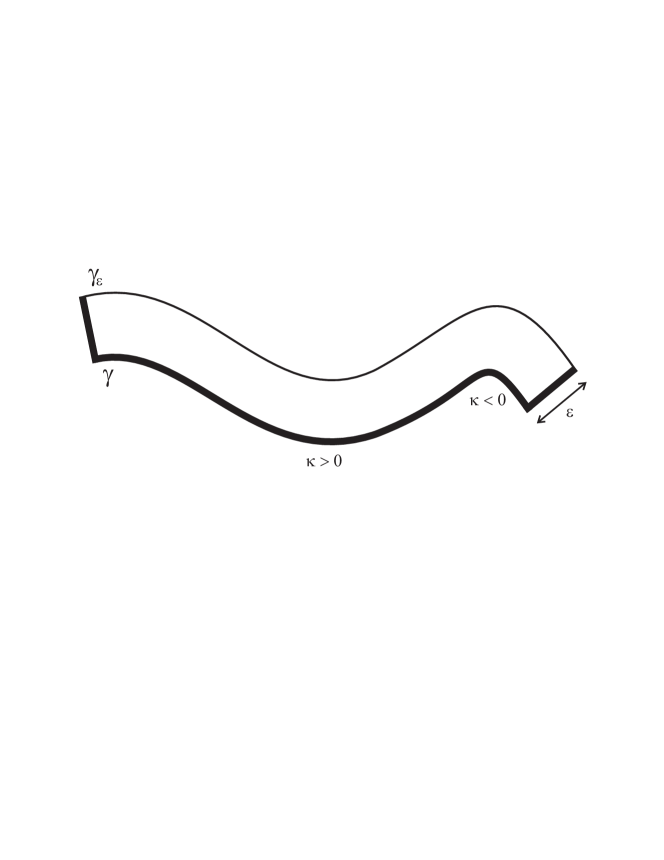
Figure 1: The geometry of the strip $\Omega_{\varepsilon}$ in a case of bounded $I$. The thick and thin lines correspond to Dirichlet and Neumann boundary conditions, respectively.

Theorem 1.1 has important consequences for the spectral properties of the operator $-\Delta_{DN}^{\Omega_{\varepsilon}}$, especially in the physically interesting situation $I=\mathbb{R}$. In this case, assuming that the curvature $\kappa$ vanishes at infinity, the leading term $\pi^{2}/(2\varepsilon)^{2}$ of (1.3) coincides with the threshold of the essential spectrum of $-\Delta_{DN}^{\Omega_{\varepsilon}}$. The next term in the expansion then tells us that

1. the discrete spectrum exists whenever $\kappa$ assumes a negative value and $\varepsilon$ is sufficiently small;

2. the number of the eigenvalues increases to infinity as $\varepsilon\to 0$.

This provides an insight into the mechanism which is behind the qualitative results obtained by Dittrich and Kříž in their 2002 letter [5]. Using $-\Delta_{DN}^{\Omega_{\varepsilon}}$ as a model for the Hamiltonian of a quantum waveguide, they show that the discrete eigenvalues exist if, and only if, the reference curve $\gamma$ of sign-definite $\kappa$ is curved “in the right direction”, namely if the Neumann boundary condition is imposed on the “locally longer” boundary (i.e. $\kappa<0$ in our setting), and that (b) holds. The results were further generalized in [21, 12], numerically tested in [24], and established in a different physical model in [17].

The purely Dirichlet or Neumann strips differ from the present situation in many respects (see [21] for a comparison). The case of the Neumann Laplacian $-\Delta_{N}^{\Omega_{\varepsilon}}$ is trivial in the sense that

$$\lambda_{1}(-\Delta_{N}^{\Omega_{\varepsilon}})=\lambda_{1}(-\Delta_{N}^{I})=0\,,$$

independently of the geometry and smallness of $\varepsilon$, where $-\Delta_{N}^{I}$ denotes the Neumann Laplacian in $L^{2}(I)$. For $j\geq 2$, one has

$$\lambda_{j}(-\Delta_{N}^{\Omega_{\varepsilon}})=\lambda_{j}(-\Delta_{N}^{I})+o(1)\qquad\mbox{as}\qquad\varepsilon\to 0\,,$$

independently of the geometry. More generally, it is well known that the spectrum of the Neumann Laplacian on an $\varepsilon$-tubular neighbourhood of a Riemannian manifold converges when $\varepsilon\to 0$ to the spectrum of the Laplace-Beltrami operator on the manifold [26].

As for the Dirichlet Laplacian $-\Delta_{D}^{\Omega_{\varepsilon}}$, it is well known [8, 15, 6, 21] that the existence of discrete spectrum in unbounded strips is robust, i.e. independent of the sign of $\kappa$. This is also reflected in the asymptotic formula, $j\geq 1$,

$$\lambda_{j}(-\Delta_{D}^{\Omega_{\varepsilon}})=\left(\frac{\pi}{\varepsilon}\right)^{2}+\lambda_{j}\big{(}-\Delta_{D}^{I}-\frac{\kappa^{2}}{4}\big{)}+o(1)\qquad\mbox{as}\qquad\varepsilon\to 0\,,$$ (1.4)

known for many years [18, 6], where $-\Delta_{D}^{I}$ denotes the Dirichlet Laplacian in $L^{2}(I)$. That is, contrary to Theorem 1.1, in the purely Dirichlet case the second term in the asymptotic expansion is independent of $\varepsilon$, always negative unless $\gamma$ is a straight line, and its value is determined by the global geometry of $\gamma$.

The local character of (1.3) rather resembles the problem of a straight narrow strip of variable width studied recently by Friedlander and Solomyak [13, 14], and also by Borisov and Freitas [1] – see also [9] for related work. In view of their asymptotics, the spectrum of the Dirichlet Laplacian is basically determined by the points where the strip is the widest. In our model the cross-section is uniform but the curvature and boundary conditions are not homogeneous.

The purely Dirichlet case with uniform cross-section differs from the present situation also in the direct method of the proof of (1.4). Using the parametrization (1.1), the spectral problem for the Laplacian $-\Delta_{D}^{\Omega_{\varepsilon}}$ in the “curved” and $\varepsilon$-dependent Hilbert space $L^{2}(\Omega_{\varepsilon})$ is transferred to the spectral problem for a more complicated operator $H_{\varepsilon}^{D}$ in $L^{2}\big{(}I\times(0,1)\big{)}$. Inspecting the dependence of the coefficients of $H_{\varepsilon}^{D}$ on $\varepsilon$, it turns out that the operator is in the limit $\varepsilon\to 0$ decoupled into a sum of the “transverse” Laplacian multiplied by $\varepsilon^{-2}$ and of the $\varepsilon$-independent Schrödinger operator on $\gamma$. At this stage, the minimax principle is sufficient to establish (1.4). Furthermore, since the “straightened” Hilbert space is independent of $\varepsilon$, it is also possible to show that (1.4) is obtained as a consequence of some sort of norm-resolvent convergence [6, 10]. An alternative approach is based on the $\Gamma$-convergence method [2]. See also [16] for a recent survey of the thin-limit problem in a wider context.

The above procedure does not work in the present situation because the transformed operator $H_{\varepsilon}^{DN}$ does not decouple as $\varepsilon\to 0$, at least at the stage of the elementary usage of the minimax principle. Moreover, the operator domain of $H_{\varepsilon}^{DN}$ becomes dependent on $\varepsilon$; contrary to the Dirichlet boundary condition, the Neumann one is transferred to an $\varepsilon$-dependent and variable Robin-type boundary condition (cf Remark 3.2 below). In this paper we propose an alternative approach, which enables us to treat the case of combined boundary conditions. Our method of proof is based on refined applications of the minimax principle.

In the following Section 2, we prove Theorem 1.1 as a consequence of upper and lower bounds to $\lambda_{j}(-\Delta_{DN}^{\Omega_{\varepsilon}})$. More specifically, these estimates imply

Theorem 1.2.

For all $j\geq 1$,

$$\lambda_{j}(-\Delta_{DN}^{\Omega_{\varepsilon}})=\left(\frac{\pi}{2\varepsilon}\right)^{2}+\lambda_{j}\big{(}-\Delta_{D}^{I}+\frac{\kappa}{\varepsilon}\big{)}+\mathcal{O}(1)\qquad\mbox{as}\qquad\varepsilon\to 0\,.$$ (1.5)

Then Theorem 1.1 follows at once as a weaker version of Theorem 1.2, by using known results about the strong-coupling/semiclassical asymptotics of eigenvalues of the one-dimensional Schrödinger operator. Indeed, for all $j\geq 1$, one has

$$\lambda_{j}\big{(}-\Delta_{D}^{I}+\frac{\kappa}{\varepsilon}\big{)}=\frac{\inf\kappa}{\varepsilon}+o(\varepsilon^{-1})\qquad\mbox{as}\qquad\varepsilon\to 0\,.$$ (1.6)

This result seems to be well known; we refer to [11, App. A] for a proof in any dimension.

Another goal of the present paper is to show that the eigenvalue convergence of Theorem 1.1 can be obtained as a consequence of the norm-resolvent “convergence” of $-\Delta_{DN}^{\Omega_{\varepsilon}}$ to $-\Delta_{D}^{I}+\kappa/\varepsilon$ as $\varepsilon\to 0$. We use the quotation marks because the latter operator is in fact $\varepsilon$-dependent and the norm-resolvent convergence should be rather interpreted as the convergence of the difference of corresponding resolvent operators in norm. However, the operators act in different Hilbert spaces and the norm-resolvent convergence still requires a meaningful reinterpretation. Because of the technical complexity, we postpone the statement of this convergence result until Section 3.

The paper is concluded by Section 4 in which we discuss possible extensions of our main results.

2 Spectral convergence

In this section we give a simple proof of Theorem 1.2 by establishing upper and lower bounds to $\lambda_{j}(-\Delta_{DN}^{\Omega_{\varepsilon}})$. We begin with necessary geometric preliminaries.

2.1 Curvilinear coordinates

As usual, the Laplacian $-\Delta_{DN}^{\Omega_{\varepsilon}}$ is introduced as the self-adjoint operator in $L^{2}(\Omega_{\varepsilon})$ associated with the quadratic form $Q_{DN}^{\Omega_{\varepsilon}}$ defined by

$$Q_{DN}^{\Omega_{\varepsilon}}[\Psi] :=\int_{\Omega_{\varepsilon}}|\nabla\Psi(x)|^{2}\,dx\,,$$

$$\Psi\in D(Q_{DN}^{\Omega_{\varepsilon}}) :=\left\{\Psi\in W^{1,2}(\Omega_{\varepsilon})\ |\quad\Psi=0\quad\mbox{on}\quad\partial\Omega_{\varepsilon}\setminus\gamma_{\varepsilon}(I)\right\}\,.$$

Here $\Psi$ on $\partial\Omega_{\varepsilon}$ is understood in the sense of traces. It is natural to express the Laplacian in the “coordinates” $(s,t)$ determined by the inverse of $\mathcal{L}_{\varepsilon}$.

As stated in Introduction, under the hypotheses that $\mathcal{L}_{\varepsilon}$ is injective and

$$\varepsilon\,\sup|\kappa|<1\,,$$ (2.1)

the mapping (1.1) induces a global diffeomorphism between $I\times(0,1)$ and $\Omega_{\varepsilon}$. This is readily seen by the inverse function theorem and the expression for the Jacobian $\det(\partial_{1}\mathcal{L}_{\varepsilon},\partial_{2}\mathcal{L}_{\varepsilon})=\varepsilon h_{\varepsilon}$ of $\mathcal{L}_{\varepsilon}$, where

$$h_{\varepsilon}(s,t):=1-\kappa(s)\,\varepsilon\,t\,.$$ (2.2)

In fact, (2.1) yields the uniform estimates

$$0<1-\varepsilon\sup\kappa\leq h_{\varepsilon}\leq 1-\varepsilon\inf\kappa<\infty\,,$$ (2.3)

where the lower bound ensures that the Jacobian never vanishes in $\overline{I}\times[0,1]$.

The passage to the natural coordinates (together with a simple scaling) is then performed via the unitary transformation

$$U_{\varepsilon}:L^{2}(\Omega_{\varepsilon})\to\mathcal{H}_{\varepsilon}:=L^{2}\big{(}I\times(0,1),h_{\varepsilon}(s,t)\,ds\,dt\big{)}:\left\{\Psi\mapsto\sqrt{\varepsilon}\ \Psi\circ\mathcal{L}_{\varepsilon}\right\}\,.$$

This leads to a unitarily equivalent operator $H_{\varepsilon}:=U_{\varepsilon}(-\Delta_{DN}^{\Omega_{\varepsilon}})U_{\varepsilon}^{-1}$ in $\mathcal{H}_{\varepsilon}$, which is associated with the quadratic form $Q_{\varepsilon}$ defined by

$$Q_{\varepsilon}[\psi] :=\int_{I\times(0,1)}\frac{|\partial_{1}\psi(s,t)|^{2}}{h_{\varepsilon}(s,t)}\,ds\,dt+\int_{I\times(0,1)}\frac{|\partial_{2}\psi(s,t)|^{2}}{\varepsilon^{2}}\,h_{\varepsilon}(s,t)\,ds\,dt\,,$$

$$\psi\in D(Q_{\varepsilon}) :=\left\{\psi\in W^{1,2}\big{(}I\times(0,1)\big{)}\ |\ \psi=0\quad\mbox{on}\quad\partial\big{(}I\times(0,1)\big{)}\setminus\big{(}I\times\{1\}\big{)}\right\}.$$

As a consequence of (2.3), $\mathcal{H}_{\varepsilon}$ and $L^{2}\big{(}I\times(0,1)\big{)}$ can be identified as vector spaces due to the equivalence of norms, denoted respectively by $\|\cdot\|_{\varepsilon}$ and $\|\cdot\|$ in the following. More precisely, we have

$$1-\varepsilon\sup\kappa\leq\frac{\|\psi\|_{\varepsilon}^{2}}{\|\psi\|^{2}}\leq 1-\varepsilon\inf\kappa\,.$$ (2.4)

That is, the fraction of norms behaves as $1+\mathcal{O}(\varepsilon)$ as $\varepsilon\to 0$.

2.2 Upper bound

Let $\psi$ be a test function from the domain $D(Q_{\varepsilon})$ of the form

$$\psi(s,t):=\varphi(s)\chi_{1}(t)\,,\qquad\mbox{where}\qquad\chi_{1}(t):=\sqrt{2}\sin\left(\pi t/2\right)$$ (2.5)

and $\varphi\in\mathop{W_{0}^{1,2}}\nolimits(I)$ is arbitrary. Note that $\chi_{1}$ is a normalized eigenfunction corresponding to the lowest eigenvalue of $-\Delta_{DN}^{(0,1)}$, i.e. the Laplacian in $L^{2}((0,1))$, subject to the Dirichlet and Neumann boundary condition at $0$ and $1$, respectively. A straightforward calculation yields

$$Q_{\varepsilon}[\psi]-\left(\frac{\pi}{2\varepsilon}\right)^{2}\|\psi\|_{\varepsilon}^{2}=\int_{I}\left(a_{\varepsilon}(s)\,|\varphi^{\prime}(s)|^{2}+\frac{\kappa(s)}{\varepsilon}\,|\varphi(s)|^{2}\right)ds\,,$$

where

$$a_{\varepsilon}(s):=\int_{0}^{1}\frac{|\chi_{1}(t)|^{2}}{h_{\varepsilon}(s,t)}\,dt\,.$$

Note that $\sup a_{\varepsilon}=1+\mathcal{O}(\varepsilon)$ due to (2.3) and the normalization of $\chi_{1}$. Using in addition the boundedness of $\kappa$ and $\|\varphi\|_{L^{2}(I)}=\|\psi\|$ together with (2.4), we can therefore write

$$\frac{Q_{\varepsilon}[\psi]}{\,\|\psi\|_{\varepsilon}^{2}}-\left(\frac{\pi}{2\varepsilon}\right)^{2}-\mathcal{O}(1)\,\leq\,\big{[}1+\mathcal{O}(\varepsilon)\big{]}\,\frac{\int_{I}\left(|\varphi^{\prime}(s)|^{2}+\frac{\kappa(s)}{\varepsilon}\,|\varphi(s)|^{2}\right)ds}{\int_{I}|\varphi(s)|^{2}\,ds}\,.$$

From this inequality, the minimax principle gives the upper bound

$$\lambda_{j}(H_{\varepsilon})-\left(\frac{\pi}{2\varepsilon}\right)^{2} \,\leq\,\big{[}1+\mathcal{O}(\varepsilon)\big{]}\,\lambda_{j}\big{(}-\Delta_{D}^{I}+\frac{\kappa}{\varepsilon}\big{)}+\mathcal{O}(1)$$

$$\,=\,\lambda_{j}\big{(}-\Delta_{D}^{I}+\frac{\kappa}{\varepsilon}\big{)}+\mathcal{O}(1)\qquad\mbox{as}\qquad\varepsilon\to 0\$$ (2.6)

for all $j\geq 1$. Here the equality follows by (1.6).

2.3 Lower bound

For all $\psi\in D(Q_{\varepsilon})$, we have

$$Q_{\varepsilon}[\psi]\geq\int_{I\times(0,1)}\frac{|\partial_{1}\psi(s,t)|^{2}}{h_{\varepsilon}(s,t)}\,ds\,dt+\int_{I\times(0,1)}\frac{\nu\big{(}\varepsilon\kappa(s)\big{)}}{\varepsilon^{2}}\ |\psi(s,t)|^{2}\,h_{\varepsilon}(s,t)\,ds\,dt\,,$$

where $\nu(\epsilon)\equiv\lambda_{1}(T_{\epsilon})$ denotes the lowest eigenvalue of the operator $T_{\epsilon}$ in the Hilbert space $L^{2}\big{(}(0,1),(1-\epsilon t)dt\big{)}$ defined by

$$(T_{\epsilon}\chi)(t) :=-\chi^{\prime\prime}(t)+\frac{\epsilon}{1-\epsilon t}\,\chi^{\prime}(t)\,,$$

$$\chi\in D(T_{\epsilon}) :=\left\{\chi\in W^{2,2}\big{(}(0,1)\big{)}\ |\quad\chi(0)=\chi^{\prime}(1)=0\right\}.$$

Note that $\nu(0)=(\pi/2)^{2}$ and that the corresponding eigenfunction for $\epsilon=0$ can be identified with $\chi_{1}$. The analytic perturbation theory yields

$$\nu(\epsilon)=\left(\frac{\pi}{2}\right)^{2}+\epsilon+\mathcal{O}\big{(}\epsilon^{2}\big{)}\qquad\mbox{as}\qquad\epsilon\to 0\,.$$ (2.7)

Using this expansion and the boundedness of $\kappa$, we can estimate

$$Q_{\varepsilon}[\psi]-\left(\frac{\pi}{2\varepsilon}\right)^{2}\|\psi\|_{\varepsilon}^{2}\geq\int_{I\times(0,1)}\left(\frac{|\partial_{1}\psi(s,t)|^{2}}{1-\varepsilon\inf\kappa}+\frac{\kappa}{\varepsilon}\,|\psi(s,t)|^{2}-C\,|\psi(s,t)|^{2}\right)ds\,dt\,,$$

where $C$ is a positive constant depending uniquely on $\|\kappa\|_{L^{\infty}(I)}$. Using in addition (2.4), we therefore get

$$\frac{Q_{\varepsilon}[\psi]}{\,\|\psi\|_{\varepsilon}^{2}}-\left(\frac{\pi}{2\varepsilon}\right)^{2}-\mathcal{O}(1)\,\geq\,\big{[}1+\mathcal{O}(\varepsilon)\big{]}\,\frac{\int_{I\times(0,1)}\left(|\partial_{1}\psi(s,t)|^{2}+\frac{\kappa(s)}{\varepsilon}\,|\psi(s,t)|^{2}\right)ds}{\int_{I\times(0,1)}|\psi(s,t)|^{2}\,ds}\,.$$

Consequently, the minimax principle gives

$$\lambda_{j}(H_{\varepsilon})-\left(\frac{\pi}{2\varepsilon}\right)^{2} \,\geq\,\big{[}1+\mathcal{O}(\varepsilon)\big{]}\,\lambda_{j}\big{(}-\Delta_{D}^{I}+\frac{\kappa}{\varepsilon}\big{)}+\mathcal{O}(1)$$

$$\,=\,\lambda_{j}\big{(}-\Delta_{D}^{I}+\frac{\kappa}{\varepsilon}\big{)}+\mathcal{O}(1)\qquad\mbox{as}\qquad\varepsilon\to 0\$$ (2.8)

for all $j\geq 1$. Again, here the equality follows by (1.6).

In view of the unitary equivalence of $H_{\varepsilon}$ with $-\Delta_{DN}^{\Omega_{\varepsilon}}$, the estimates (2.2) and (2.3) prove Theorem 1.2.

3 Norm-resolvent convergence

In this section we study the mechanism which is behind the eigenvalue convergence of Theorem 1.1 in more details. First we explain what we mean by the norm-resolvent convergence of the family of operators $\{-\Delta_{DN}^{\Omega_{\varepsilon}}\}_{\varepsilon>0}$.

3.1 The reference Hilbert space and the result

In Section 2.1, we identified the Laplacian $-\Delta_{DN}^{\Omega_{\varepsilon}}$ with a Laplace-Beltrami-type operator $H_{\varepsilon}$ in $\mathcal{H}_{\varepsilon}$. Now it is more convenient to pass to another unitarily equivalent operator $\hat{H}_{\varepsilon}$ which acts in the “fixed” (i.e. $\varepsilon$-independent) Hilbert space

$$\mathcal{H}_{0}:=L^{2}\big{(}I\times(0,1)\big{)}\,.$$

This is enabled by means of the unitary mapping

$$\hat{U}_{\varepsilon}:\mathcal{H}_{\varepsilon}\to\mathcal{H}_{0}:\big{\{}\psi\mapsto\sqrt{h_{\varepsilon}}\ \psi\big{\}}\,,$$

provided that the curvature $\kappa$ is differentiable in a weak sense; henceforth we assume that

$$\kappa^{\prime}\in L^{\infty}(I)\,.$$ (3.1)

We set $\hat{H}_{\varepsilon}:=\hat{U}_{\varepsilon}H_{\varepsilon}\hat{U}_{\varepsilon}^{-1}$. As a comparison operator to $\hat{H}_{\varepsilon}$ for small $\varepsilon$, we consider the decoupled operator

$$\hat{H}_{0}:=\left(-\Delta_{D}^{I}+\frac{\kappa}{\varepsilon}\right)\otimes 1+1\otimes\Big{(}-\frac{1}{\varepsilon^{2}}\,\Delta_{DN}^{(0,1)}\Big{)}\qquad\mbox{in}\qquad L^{2}(I)\otimes L^{2}\big{(}(0,1)\big{)}\,.$$

Here the subscript $0$ is just a notational convention, of course, since $\hat{H}_{0}$ still depends on $\varepsilon$. Using natural isomorphisms, we may reconsider $\hat{H}_{0}$ as an operator in $\mathcal{H}_{0}$.

We clearly have

$$\hat{H}_{0}\geq\left(\frac{\pi}{2\varepsilon}\right)^{2}+\frac{\inf\kappa}{\varepsilon}\,.$$ (3.2)

At the same time,

$$\hat{H}_{\varepsilon}\geq\frac{\nu(\varepsilon\kappa)}{\varepsilon^{2}}\geq\frac{\nu(\varepsilon\inf\kappa)}{\varepsilon^{2}}=\left(\frac{\pi}{2\varepsilon}\right)^{2}+\frac{\inf\kappa}{\varepsilon}+\mathcal{O}(1)\,,$$ (3.3)

where the first inequality was established (for the unitarily equivalent operator $H_{\varepsilon}$) in the beginning of Section 2.3, the second inequality holds due to the monotonicity of $\varepsilon\mapsto\nu(\varepsilon)$ proved in [12, Thm. 2] and the equality follows from (2.7). (Alternatively, we could use Theorem 1.1 to get (3.3), however, one motivation of the present section is to show that the former can be obtained as a consequence of Theorem 3.1 below.) Fix any number

$$k>-\inf\kappa\,.$$ (3.4)

It follows that $\hat{H}_{\varepsilon}-\pi^{2}/(2\varepsilon)^{2}+k/\varepsilon$ and $\hat{H}_{0}-\pi^{2}/(2\varepsilon)^{2}+k/\varepsilon$ are positive operators for all sufficiently small $\varepsilon$.

Now we are in a position to state the main result of this section.

Theorem 3.1.

In addition to the injectivity of $\mathcal{L}_{\varepsilon}$ and the boundedness of $\kappa$, let us assume (3.1). Then there exist positive constants $\varepsilon_{0}$ and $C_{0}$, depending uniquely on $k$ and the supremum norms of $\kappa$ and $\kappa^{\prime}$, such that for all $\varepsilon\in(0,\varepsilon_{0})$:

$$\left\|\left[\hat{H}_{\varepsilon}-\left(\frac{\pi}{2\varepsilon}\right)^{2}+\frac{k}{\varepsilon}\right]^{-1}-\left[\hat{H}_{0}-\left(\frac{\pi}{2\varepsilon}\right)^{2}+\frac{k}{\varepsilon}\right]^{-1}\right\|\ \leq\ C_{0}\,\varepsilon^{3/2}\,.$$

The theorem is proved in several steps divided into the following subsections. In particular, it follows as a direct consequence of Lemmata 3.3 and 3.4 below. In the final subsection we show how it implies the convergence of eigenvalues of Theorem 1.1.

3.2 The transformed Laplacian

Let us now find an explicit expression for the quadratic form $\hat{Q}_{\varepsilon}$ associated with the operator $\hat{H}_{\varepsilon}$. By definition, it is given by

$$\hat{Q}_{\varepsilon}[\psi]:=Q_{\varepsilon}[\hat{U}_{\varepsilon}^{-1}\psi]\,,\qquad\psi\in D(\hat{Q}_{\varepsilon}):=\hat{U}_{\varepsilon}D(Q_{\varepsilon})\,.$$

One easily verifies that

$$D(\hat{Q}_{\varepsilon})=D(Q_{\varepsilon})=:\mathcal{Q}\,,$$ (3.5)

which is actually independent of $\varepsilon$. Furthermore, for any $\psi\in\mathcal{Q}$, we have

$$\hat{Q}_{\varepsilon}[\psi]=\hat{Q}_{\varepsilon}^{1}[\psi]+\hat{Q}_{\varepsilon}^{2}[\psi]\,,$$

where

$$\hat{Q}_{\varepsilon}^{1}[\psi] :=\int\frac{\big{|}\partial_{1}(h_{\varepsilon}^{-1/2}\psi)\big{|}^{2}}{h_{\varepsilon}} = \int\left\{\frac{|\partial_{1}\psi|^{2}}{h_{\varepsilon}^{2}}+V_{\varepsilon}^{1}\,|\psi|^{2}+V_{\varepsilon}^{2}\,\Re\big{(}\overline{\psi}\partial_{1}\psi\big{)}\right\},$$

$$\hat{Q}_{\varepsilon}^{2}[\psi] :=\int\frac{\big{|}\partial_{2}(h_{\varepsilon}^{-1/2}\psi)\big{|}^{2}}{\varepsilon^{2}}\ h_{\varepsilon} = \int\left\{\frac{|\partial_{2}\psi|^{2}}{\varepsilon^{2}}+V_{\varepsilon}^{3}\,|\psi|^{2}+V_{\varepsilon}^{4}\,\Re\big{(}\overline{\psi}\partial_{2}\psi\big{)}\right\},$$

with

$$V_{\varepsilon}^{1}(s,t) :=\frac{1}{4}\frac{\kappa^{\prime}(s)^{2}\varepsilon^{2}t^{2}}{h_{\varepsilon}(s,t)^{4}}\,, V_{\varepsilon}^{2}(s,t) :=\frac{\kappa^{\prime}(s)\varepsilon t}{h_{\varepsilon}(s,t)^{3}}\,,$$

$$V_{\varepsilon}^{3}(s,t) :=\frac{1}{4}\frac{\kappa(s)^{2}}{h_{\varepsilon}(s,t)^{2}}\,, V_{\varepsilon}^{4}(s,t) :=\frac{\kappa(s)}{\varepsilon h_{\varepsilon}(s,t)}\,.$$

Here and in the sequel the integral sign $\int$ refers to an integration over $I\times(0,1)$. Integrating by parts in the expression for $\hat{Q}_{\varepsilon}^{2}[\psi]$, we finally arrive at

$$\hat{Q}_{\varepsilon}[\psi]=\int\left\{\frac{|\partial_{1}\psi|^{2}}{h_{\varepsilon}^{2}}+\frac{|\partial_{2}\psi|^{2}}{\varepsilon^{2}}+(V_{\varepsilon}^{1}-V_{\varepsilon}^{3})|\psi|^{2}+V_{\varepsilon}^{2}\,\Re\big{(}\overline{\psi}\partial_{1}\psi\big{)}\right\}+\int_{\partial}v_{\varepsilon}\,|\psi|^{2}\,,$$

where

$$v_{\varepsilon}(s,t):=\frac{1}{2}\frac{\kappa(s)}{\varepsilon\big{(}1-\varepsilon\kappa(s)\big{)}}\,.$$

Here and in the sequel the integral sign $\int_{\partial}$ refers to an integration over the boundary $I\times\{1\}$.

Remark 3.2.

$\hat{H}_{\varepsilon}$ is exactly the operator $H_{\varepsilon}^{DN}$ mentioned briefly in Introduction. Let us remark in this context that, contrary to the form domains (3.5), the operator domains of $H_{\varepsilon}$ and $\hat{H}_{\varepsilon}$ do differ (unless the curvature $\kappa$ vanishes identically). Indeed, under additional regularity conditions about $\gamma$, it can be shown that while functions from $D(H_{\varepsilon})$ satisfy Neumann boundary conditions on $I\times\{1\}$, the functions $\psi$ from $D(\hat{H}_{\varepsilon})$ satisfy non-homogeneous Robin-type boundary conditions $\partial_{2}\psi+\varepsilon^{2}v_{\varepsilon}\psi=0$ on $I\times\{1\}$. This is the reason why the decoupling of $\hat{H}_{\varepsilon}$ for small $\varepsilon$ is not obvious in this situation. At the same time, we see that the operator domain of $\hat{H}_{\varepsilon}$ heavily depends on the geometry of $\gamma$. For our purposes, however, it will be enough to work with the associated quadratic form $\hat{Q}_{\varepsilon}$ whose domain is independent of $\varepsilon$ and $\kappa$.

3.3 Renormalized operators and resolvent bounds

It will be more convenient to work with the shifted operators

$$L_{\varepsilon}:=\hat{H}_{\varepsilon}-\left(\frac{\pi}{2\varepsilon}\right)^{2}+\frac{k}{\varepsilon}\qquad\mbox{and}\qquad L_{0}:=\hat{H}_{0}-\left(\frac{\pi}{2\varepsilon}\right)^{2}+\frac{k}{\varepsilon}\,.$$

Let $l_{\varepsilon}$ and $l_{0}$ denote the associated quadratic forms. It is important that they have the same domain $\mathcal{Q}$. More precisely, $\hat{H}_{0}$ was initially defined as a direct sum, however, using natural isomorphisms, it is clear that we can identify the form domain of $L_{0}$ with $\mathcal{Q}$ and

$$l_{0}[\psi]=\int\left\{|\partial_{1}\psi|^{2}+\frac{1}{\varepsilon^{2}}\Big{[}|\partial_{2}\psi|^{2}-\left(\frac{\pi}{2}\right)^{2}|\psi|^{2}\Big{]}+\frac{k+\kappa}{\varepsilon}\,|\psi|^{2}\right\}$$

for all $\psi\in\mathcal{Q}$.

It will be also useful to have an intermediate operator $L$, obtained from $L_{\varepsilon}$ after neglecting its non-singular dependence on $\varepsilon$ but keeping the boundary term. For simplicity, henceforth we assume that $\varepsilon$ is less than one and that it is in fact so small that (2.1) holds with a number less than one on the right hand side. Consequently,

$$|h_{\varepsilon}-1|\leq C\varepsilon\,,\ |V_{\varepsilon}^{1}|\leq C\varepsilon^{2}\,,\ |V_{\varepsilon}^{2}|\leq C\varepsilon\,,\ |V_{\varepsilon}^{3}|\leq C\,,\ |V_{\varepsilon}^{4}|\leq C\varepsilon^{-1}\,,\ |v_{\varepsilon}|\leq C\varepsilon^{-1}\,.$$ (3.6)

Here and in the sequel, we use the convention that $C$ and $c$ are positive constants which possibly depend on $k$ and the supremum norms of $\kappa$ and $\kappa^{\prime}$, and which may vary from line to line. In view of these estimates, it is reasonable to introduce $L$ as the operator associated with the quadratic form $l$ defined by $D(l):=\mathcal{Q}$ and

$$l[\psi]:=\int\left\{|\partial_{1}\psi|^{2}+\frac{1}{\varepsilon^{2}}\Big{[}|\partial_{2}\psi|^{2}-\left(\frac{\pi}{2}\right)^{2}|\psi|^{2}\Big{]}+\frac{k}{\varepsilon}\,|\psi|^{2}\right\}+\int_{\partial}v_{\varepsilon}\,|\psi|^{2}$$

for all $\psi\in\mathcal{Q}$. Indeed, it follows from (3.6) that

$$\big{|}l_{\varepsilon}[\psi]-l[\psi]\big{|} \leq\int\Big{\{}|h_{\varepsilon}^{-2}-1||\partial_{1}\psi|^{2}+|V_{\varepsilon}^{1}-V_{\varepsilon}^{3}||\psi|^{2}+|V_{\varepsilon}^{2}|\,|\psi||\partial_{1}\psi|\Big{\}}$$

$$\leq C\big{(}\varepsilon\|\partial_{1}\psi\|^{2}+\|\psi\|^{2}\big{)}$$ (3.7)

for all $\psi\in\mathcal{Q}$.

Let us now argue that, for every $\psi\in\mathcal{Q}$ and for all sufficiently small $\varepsilon$ (which precisely means that $\varepsilon$ has to be less than an explicit constant depending on $k$ and the supremum norms of $\kappa$ and $\kappa^{\prime}$), we have

$$\min\left\{l_{\varepsilon}[\psi],l_{0}[\psi],l[\psi]\right\}\geq c\,\left(\|\partial_{1}\psi\|^{2}+\varepsilon^{-1}\|\psi\|^{2}\right)\,.$$ (3.8)

Here the bound for $l_{0}$ follows at once by improving the crude bound (3.2) and recalling (3.4). The bound for $l$ follows from that for $l_{\varepsilon}$ and from (3.3). As for the bound for $l_{\varepsilon}$, we first remark that the estimates (3.3) actually hold for the part of $\hat{H}_{\varepsilon}$ associated with $\hat{Q}_{\varepsilon}^{2}$. Second, using (3.6) and some elementary estimates, we have $\hat{Q}_{\varepsilon}^{1}[\psi]\geq(c-C\varepsilon)\|\partial_{1}\psi\|^{2}-C\|\psi\|^{2}$. Hence, for $\varepsilon$ small enough, we indeed conclude with the bound for $l_{\varepsilon}$.

The estimates (3.8) imply that, for all sufficiently small $\varepsilon$,

$$\|L_{\varepsilon}^{-1}\|\leq C\varepsilon\,,\qquad\|L_{0}^{-1}\|\leq C\varepsilon\,,\qquad\|L^{-1}\|\leq C\varepsilon\,.$$ (3.9)

3.4 An intermediate convergence result

As the first step in the proof of Theorem 3.1, we show that it is actually enough to establish the norm-resolvent convergence for a simpler operator $L$ instead of $L_{\varepsilon}$.

Lemma 3.3.

Under the assumptions of Theorem 3.1, there exist positive constants $\varepsilon_{0}$ and $C_{0}$, depending uniquely on $k$ and the supremum norms of $\kappa$ and $\kappa^{\prime}$, such that for all $\varepsilon\in(0,\varepsilon_{0})$:

$$\left\|L_{\varepsilon}^{-1}-L^{-1}\right\|\ \leq\ C_{0}\,\varepsilon^{2}\,.$$

Proof.

We are inspired by [13, Sec. 3]. Adapting the estimate (3.3) for the sesquilinear form generated by $l_{\varepsilon}-l$ and using (3.8), we get

$$\big{|}l_{\varepsilon}(\phi,\psi)-l(\phi,\psi)\big{|} \leq C\sqrt{\varepsilon\|\partial_{1}\phi\|^{2}+\|\phi\|^{2}}\sqrt{\varepsilon\|\partial_{1}\psi\|^{2}+\|\psi\|^{2}}$$

$$\leq(C/c)\,\varepsilon\sqrt{l[\phi]\,l_{\varepsilon}[\psi]}$$

for every $\phi,\psi\in\mathcal{Q}$. Choosing $\phi:=L^{-1}f$ and $\psi:=L_{\varepsilon}^{-1}g$, where $f,g\in\mathcal{H}_{0}$ are arbitrary, we arrive at

$$\big{|}(f,L^{-1}g)-(f,L_{\varepsilon}^{-1}g)\big{|}\leq(C/c)\,\varepsilon\sqrt{(f,L^{-1}f)(g,L_{\varepsilon}^{-1}g)}\leq(C^{2}/c)\,\varepsilon^{2}\,\|f\|\,\|g\|\,.$$

Here $(\cdot,\cdot)$ denotes the inner product in $\mathcal{H}_{0}$ and the second inequality follows from (3.9). This completes the proof with $C_{0}:=C^{2}/c$. ∎

3.5 An orthogonal decomposition of the Hilbert space

Contrary to Lemma 3.3, the convergence of $\|L^{-1}-L_{0}^{-1}\|$ is less obvious. We follow the idea of [13] and decompose the Hilbert space $\mathcal{H}_{0}$ into an orthogonal sum

$$\mathcal{H}_{0}=\mathfrak{H}_{1}\oplus\mathfrak{H}_{1}^{\bot}\,,$$

where the subspace $\mathfrak{H}_{1}$ consists of functions $\psi_{1}$ such that

$$\psi_{1}(s,t)=\varphi_{1}(s)\chi_{1}(t)\,.$$ (3.10)

Recall that $\chi_{1}$ has been introduced in (2.5). Since $\chi_{1}$ is normalized, we clearly have $\|\psi_{1}\|=\|\varphi_{1}\|_{L^{2}(I)}$. Given any $\psi\in\mathcal{H}_{0}$, we have the decomposition

$$\psi=\psi_{1}+\psi_{\bot}\qquad\mbox{with}\qquad\psi_{1}\in\mathfrak{H}_{1},\ \psi_{\bot}\in\mathfrak{H}_{1}^{\bot}\,,$$ (3.11)

where $\psi_{1}$ has the form (3.10) with $\varphi_{1}(s):=\int_{0}^{1}\psi(s,t)\chi_{1}(t)dt$. Note that $\psi_{1}\in\mathcal{Q}$ if $\psi\in\mathcal{Q}$. The inclusion $\psi_{\bot}\in\mathfrak{H}_{1}^{\bot}$ means that

$$\int_{0}^{1}\psi_{\bot}(s,t)\,\chi_{1}(t)\,dt=0\qquad\mbox{for a.e.}\quad s\in I\,.$$ (3.12)

If in addition $\psi_{\bot}\in\mathcal{Q}$, then one can differentiate the last identity to get

$$\int_{0}^{1}\partial_{1}\psi_{\bot}(s,t)\,\chi_{1}(t)\,dt=0\qquad\mbox{for a.e.}\quad s\in I\,.$$ (3.13)

3.6 A complementary convergence result

Now we are in a position to prove the following result, which together with Lemma 3.3 establishes Theorem 3.1.

Lemma 3.4.

Under the assumptions of Theorem 3.1, there exist positive constants $\varepsilon_{0}$ and $C_{0}$, depending uniquely on $k$ and the supremum norms of $\kappa$ and $\kappa^{\prime}$, such that for all $\varepsilon\in(0,\varepsilon_{0})$:

$$\left\|L^{-1}-L_{0}^{-1}\right\|\ \leq\ C_{0}\,\varepsilon^{3/2}\,.$$

Proof.

Again, we use some of the ideas of [13, Sec. 3]. As a consequence of (3.12) and (3.13), we get that $l_{0}(\psi_{1},\psi_{\bot})=0$; therefore

$$l_{0}[\psi]=l_{0}[\psi_{1}]+l_{0}[\psi_{\bot}]$$ (3.14)

for every $\psi\in\mathcal{Q}$. At the same time, for sufficiently small $\varepsilon$,

$$l_{0}[\psi_{1}] \geq c\left(\|\varphi_{1}^{\prime}\|_{L^{2}(I)}^{2}+\varepsilon^{-1}\,\|\varphi_{1}\|_{L^{2}(I)}^{2}\right)\,,$$ (3.15)

$$l_{0}[\psi_{\bot}] \geq c\Big{(}\|\partial_{1}\psi_{\bot}\|^{2}+\varepsilon^{-2}\,\|\partial_{2}\psi_{\bot}\|^{2}+\varepsilon^{-2}\,\|\partial\psi_{\bot}\|^{2}\Big{)}\,,$$

where the second inequality is based on $\int|\partial_{2}\psi_{\bot}|^{2}\geq\pi^{2}\int|\psi_{\bot}|^{2}$.

Let us now compare $l_{0}$ with $l$. For every $\psi\in\mathcal{Q}$, we define

$$m[\psi]:=l[\psi]-l_{0}[\psi]=\int_{\partial}v_{\varepsilon}\,|\psi|^{2}-\int\frac{\kappa}{\varepsilon}\,|\psi|^{2}\,.$$

Using the estimates (3.6) and (3.15), we get, for any $\psi\in\mathcal{Q}$ decomposed as in (3.11),

$$m[\psi_{1}] =\int_{I}\frac{\kappa(s)^{2}}{1-\varepsilon\kappa(s)}\,|\varphi_{1}(s)|^{2}ds\leq C\,\|\varphi_{1}\|_{L^{2}(\mathbb{R})}^{2}\leq(C/c)\,\varepsilon\,l_{0}[\psi_{1}]\,,$$

$$|m[\psi_{\bot}]| \leq C\varepsilon^{-1}\Big{(}\|\psi_{\bot}\|\|\partial_{2}\psi_{\bot}||+\|\psi_{\bot}\|^{2}\Big{)}\leq 2(C/c)\,\varepsilon\,l_{0}[\psi_{\bot}]\,,$$

$$|m(\psi_{1},\psi_{\bot})| =\left|\int_{\partial}v_{\varepsilon}\,\overline{\psi_{1}}\psi_{\bot}\right|\leq C\varepsilon^{-1}\|\psi_{1}\|\sqrt{\|\psi_{\bot}\|\|\partial_{2}\psi_{\bot}||}$$

$$\leq(C/c)\,\varepsilon^{1/2}\sqrt{l_{0}[\psi_{1}]l_{0}[\psi_{\bot}]}\,.$$

Except for $m[\psi_{1}]$, here the boundary integral was estimated via

$$\int_{\partial}|\psi|^{2}=\int\partial_{2}|\psi|^{2}=\int 2\,\Re\big{(}\overline{\psi}\partial_{2}\psi\big{)}\leq 2\,\|\psi\|\,\|\partial_{2}\psi\|\,.$$

Taking (3.14) into account, we conclude with the estimate (which can be again adapted for the corresponding sesquilinear form)

$$|m[\psi]|\leq C\,\varepsilon^{1/2}\ l_{0}[\psi]$$

valid for every $\psi\in\mathcal{Q}$ and all sufficiently small $\varepsilon$. In particular, this implies the crude estimates

$$c\,l_{0}[\psi]\leq l[\psi]\leq C\,l_{0}[\psi]\,.$$

Summing up, we have the crucial bound

$$\big{|}l(\phi,\psi)-l_{0}(\phi,\psi)\big{|}\leq C\,\varepsilon^{1/2}\,\sqrt{l_{0}[\phi]\,l[\psi]}\,,$$

valid for arbitrary $\phi,\psi\in\mathcal{Q}$. The rest of the proof then follows the lines of the proof of Lemma 3.3. ∎

3.7 Convergence of eigenvalues

As an application of Theorem 3.1, we shall show now how it implies the eigenvalue asymptotics of Theorem 1.1. Recall that the numbers $\lambda_{j}(H)$ represent either eigenvalues below the essential spectrum or the threshold of the essential spectrum of $H$. In particular, they provide a complete information about the spectrum of $H$ if it is an operator with compact resolvent. In our situation, this will be the case if $I$ is bounded, but let us stress that we allow infinite or semi-infinite intervals, too.

We begin with analysing the spectrum of the comparison operator.

Lemma 3.5.

Let $\kappa$ be bounded. One has

$$\lambda_{1}(\hat{H}_{0})=\lambda_{1}\big{(}-\Delta_{D}^{I}+\frac{\kappa}{\varepsilon}\big{)}+\left(\frac{\pi}{2\varepsilon}\right)^{2}\,.$$

Moreover, for any integer $N\geq 2$, there exists a positive constant $\varepsilon_{0}$ depending on $N$, $\kappa$ and $I$ such that for all $\varepsilon<\varepsilon_{0}$:

$$\forall j\in\{1,\dots,N\},\qquad\lambda_{j}(\hat{H}_{0})=\lambda_{j}\big{(}-\Delta_{D}^{I}+\frac{\kappa}{\varepsilon}\big{)}+\left(\frac{\pi}{2\varepsilon}\right)^{2}\,.$$

Proof.

Since $\hat{H}_{0}$ is decoupled, we know that (cf [25, Corol. of Thm. VIII.33])

$$\left\{\lambda_{j}(\hat{H}_{0})\right\}_{j=1}^{\infty}=\left\{\lambda_{j}\big{(}-\Delta_{D}^{I}+\frac{\kappa}{\varepsilon}\big{)}\right\}_{j=1}^{\infty}+\left\{\left(\frac{j\pi}{2\varepsilon}\right)^{2}\right\}_{j=1}^{\infty}\,,$$

and it only remains to arrange the sum of the numbers on the right hand side into a non-decreasing sequence. The assertion for $N=1$ is therefore trivial. Let $j\geq 2$ and assume by induction that $\lambda_{j-1}(\hat{H}_{0})-\pi^{2}/(2\varepsilon)^{2}=\lambda_{j-1}(-\Delta_{D}^{I}+\kappa/\varepsilon)$. Then

$$\lambda_{j}(\hat{H}_{0})-\pi^{2}/(2\varepsilon)^{2}=\min\left\{\lambda_{j-1}(-\Delta_{D}^{I}+\kappa/\varepsilon),3\pi^{2}/(2\varepsilon)^{2}\right\}$$

and the assertion of Lemma follows at once due to the asymptotics (1.6). ∎

Now, fix $j\geq 1$ and assume that $\varepsilon$ is so small that the conclusions of Theorem 3.1 and Lemma 3.5 hold. By virtue of Theorem 3.1, we have

$$\left|\left[\lambda_{j}(\hat{H}_{\varepsilon})-\left(\frac{\pi}{2\varepsilon}\right)^{2}+\frac{k}{\varepsilon}\right]^{-1}-\left[\lambda_{j}(\hat{H}_{0})-\left(\frac{\pi}{2\varepsilon}\right)^{2}+\frac{k}{\varepsilon}\right]^{-1}\right|\ \leq\ C_{0}\,\varepsilon^{3/2}\,,$$

since the left hand side is estimated by the norm of the resolvent difference. Using now Lemma 3.5, the above estimate is equivalent to

$$\left|\frac{1}{\varepsilon\big{[}\lambda_{j}(\hat{H}_{\varepsilon})-\pi^{2}/(2\varepsilon)^{2}\big{]}+k}-\frac{1}{\varepsilon\,\lambda_{j}(-\Delta_{D}^{I}+\kappa/\varepsilon)+k}\right|\ \leq\ C_{0}\,\varepsilon^{1/2}\,.$$ (3.16)

Consequently, recalling (1.6), we conclude with

$$\lim_{\varepsilon\to 0}\varepsilon\left[\lambda_{j}(\hat{H}_{\varepsilon})-\left(\frac{\pi}{2\varepsilon}\right)^{2}\right]=\lim_{\varepsilon\to 0}\varepsilon\,\lambda_{j}\big{(}-\Delta_{D}^{I}+\frac{\kappa}{\varepsilon}\big{)}=\inf\kappa\,.$$

This is indeed equivalent to Theorem 1.1 because $\hat{H}_{\varepsilon}$ and $-\Delta_{DN}^{\Omega_{\varepsilon}}$ are unitarily equivalent (therefore isospectral).

Remark 3.6.

Because of the lack of one half in the power of $\varepsilon$ in Theorem 3.1, it turns out that (3.16) yields a slightly worse result than Theorem 1.2. Let us also emphasize that Theorem 1.1 and 1.2 have been proved in Section 2 without the need to assume the extra condition (3.1). On the other hand, Theorem 3.1 contains an operator-type convergence result of independent interest.

4 Possible extensions

4.1 Different boundary conditions

The result of Theorem 1.2 readily extends to the case of other boundary conditions imposed on the sides $\mathcal{L}_{\varepsilon}\big{(}\{\inf I\}\times(0,1)\big{)}$ and $\mathcal{L}_{\varepsilon}\big{(}\{\sup I\}\times(0,1)\big{)}$, provided that the boundary conditions for the one-dimensional Schrödinger operator are changed accordingly.

It is more interesting to impose different boundary conditions on the approaching parallel curves as $\varepsilon\to 0$. As an example, let us keep the Dirichlet boundary conditions but replace the Neumann boundary condition by the Robin condition of the type

$$\frac{\partial\Psi}{\partial n}+(\alpha\circ\ell_{\varepsilon}^{-1})\,\Psi=0\qquad\mbox{on}\qquad\gamma_{\varepsilon}(I)\,.$$

Here $\ell_{\varepsilon}:=\mathcal{L}_{\varepsilon}(\cdot,1)$ and $\alpha:I\to\mathbb{R}$ is assumed to be bounded and uniformly continuous. Let us denote the corresponding Laplacian by $-\Delta_{DR_{\alpha}}^{\Omega_{\varepsilon}}$. Then the method of the present paper gives

Theorem 4.1.

For all $j\geq 1$,

$$\lambda_{j}(-\Delta_{DR_{\alpha}}^{\Omega_{\varepsilon}}) =\left(\frac{\pi}{2\varepsilon}\right)^{2}+\lambda_{j}\big{(}-\Delta_{D}^{I}+\frac{\kappa+2\alpha}{\varepsilon}\big{)}+\mathcal{O}(1)$$

$$=\left(\frac{\pi}{2\varepsilon}\right)^{2}+\frac{\inf(\kappa+2\alpha)}{\varepsilon}+o(\varepsilon^{-1})\qquad\mbox{as}\qquad\varepsilon\to 0\,.$$

Let us mention that strips with this combination of Dirichlet and Robin boundary conditions were studied in [12].

4.2 Higher-dimensional generalization

Let $\Omega_{\varepsilon}$ be a three-dimensional layer instead of the planar strip. That is, we keep the definition (1.2) with (1.1), but now $\gamma:I\subseteq\mathbb{R}^{2}\to\mathbb{R}^{3}$ is a parametrization of a two-dimensional surface embedded in $\mathbb{R}^{3}$ and $n:=(\partial_{1}\gamma)\times(\partial_{2}\gamma)$, where the cross denotes the vector product in $\mathbb{R}^{3}$. Let $M$ be the corresponding mean curvature. Proceeding in the same way as in Section 2 (we omit the details but refer to [7] for a necessary geometric background), we get

Theorem 4.2.

For all $j\geq 1$,

$$\lambda_{j}(-\Delta_{DN}^{\Omega_{\varepsilon}}) =\left(\frac{\pi}{2\varepsilon}\right)^{2}+\lambda_{j}\big{(}-\Delta_{D}^{\gamma}+\frac{2M}{\varepsilon}\big{)}+\mathcal{O}(1)$$

$$=\left(\frac{\pi}{2\varepsilon}\right)^{2}+\frac{2\inf M}{\varepsilon}+o(\varepsilon^{-1})\qquad\mbox{as}\qquad\varepsilon\to 0\,,$$

where $-\Delta_{D}^{\gamma}$ denotes the Laplace-Beltrami operator in $L^{2}\big{(}\gamma(I)\big{)}$, subject to Dirichlet boundary conditions.

Notice that the leading geometric term in the asymptotic expansions depends on the extrinsic curvature only. This suggests that the spectral properties of the Dirichlet-Neumann layers will differ significantly from the purely Dirichlet case studied in [7, 3, 22, 23], where the Gauss curvature of $\gamma$ plays a crucial role.

4.3 Curved ambient space

The results of the present paper extend to the case of strips embedded in an abstract two-dimensional Riemannian manifold $\mathcal{A}$ instead of the Euclidean plane. Indeed, it follows from [19] (see also [20] and [10, Sec. 5]) that the quadratic form $Q_{\varepsilon}$ has the same structure; the only difference is that in this more general situation $h_{\varepsilon}$ is obtained as the solution of the Jacobi equation

$$\partial_{2}^{2}h_{\varepsilon}+\varepsilon^{2}\,K\,h_{\varepsilon}=0\qquad\textrm{with}\qquad\left\{\begin{aligned} h_{\varepsilon}(\cdot,0)&=1\,,\\ \partial_{2}h_{\varepsilon}(\cdot,0)&=-\varepsilon\,\kappa\,,\end{aligned}\right.$$

where $K$ is the Gauss curvature of $\mathcal{A}$. Here $\kappa$ is the curvature of $\gamma:I\to\mathcal{A}$ (it is in fact the geodesic curvature of $\gamma$ if the ambient space $\mathcal{A}$ is embedded in $\mathbb{R}^{3}$). Consequently, up to higher-order terms in $\varepsilon$, the function $h_{\varepsilon}$ coincides with the expression (2.2) for the flat case $K=0$. Namely,

$$h_{\varepsilon}(s,t)=1-\kappa(s)\,\varepsilon\,t+\mathcal{O}(\varepsilon^{2})\qquad\mbox{as}\qquad\varepsilon\to 0\,.$$

Following the lines of the proof in Section 2, it is then possible to check that Theorems 1.1 and 1.2 remain valid without changes. The curvature of the ambient space comes into the asymptotics via higher-order terms only.

Acknowledgment

The work has been supported by the Czech Academy of Sciences and its Grant Agency within the projects IRP AV0Z10480505 and A100480501, and by the project LC06002 of the Ministry of Education, Youth and Sports of the Czech Republic.

References

- [1] D. Borisov and P. Freitas, Singular asymptotic expansions for Dirichlet eigenvalues and eigenfunctions of the Laplacian on thin planar domains, Ann. Inst. H. Poincaré Anal. Non Linéaire, to appear; preprint on arXiv:0712.3245v1 [math.SP] (2007).
- [2] G. Bouchitté, M. L. Mascarenhas, and L. Trabucho, On the curvature and torsion effects in one dimensional waveguides, Control, Optimisation and Calculus of Variations 13 (2007), no. 4, 793–808.
- [3] G. Carron, P. Exner, and D. Krejčiřík, Topologically nontrivial quantum layers, J. Math. Phys. 45 (2004), 774–784.
- [4] E. B. Davies, Spectral theory and differential operators, Camb. Univ Press, Cambridge, 1995.
- [5] J. Dittrich and J. Kříž, Curved planar quantum wires with Dirichlet and Neumann boundary conditions, J. Phys. A 35 (2002), L269–275.
- [6] P. Duclos and P. Exner, Curvature-induced bound states in quantum waveguides in two and three dimensions, Rev. Math. Phys. 7 (1995), 73–102.
- [7] P. Duclos, P. Exner, and D. Krejčiřík, Bound states in curved quantum layers, Commun. Math. Phys. 223 (2001), 13–28.
- [8] P. Exner and P. Šeba, Bound states in curved quantum waveguides, J. Math. Phys. 30 (1989), 2574–2580.
- [9] P. Freitas, Precise bounds and asymptotics for the first Dirichlet eigenvalue of triangles and rhombi, J. Funct. Anal. 251 (2007), 376–398.
- [10] P. Freitas and D. Krejčiřík, Location of the nodal set for thin curved tubes, Indiana Univ. Math. J. 57 (2008), no. 1, to appear; preprint on [math.SP/0602470] (2006).
- [11] , Instability results for the damped wave equation in unbounded domains, J. Differential Equations 211 (2005), no. 1, 168–186.
- [12] , Waveguides with combined Dirichlet and Robin boundary conditions, Math. Phys. Anal. Geom. 9 (2006), no. 4, 335–352.
- [13] L. Friedlander and M. Solomyak, On the spectrum of the Dirichlet Laplacian in a narrow strip, preprint on arXiv:0705.4058v1 [math.SP] (2007).
- [14] , On the spectrum of the Dirichlet Laplacian in a narrow strip, II, preprint on arXiv:0710.1886v1 [math.SP] (2007).
- [15] J. Goldstone and R. L. Jaffe, Bound states in twisting tubes, Phys. Rev. B 45 (1992), 14100–14107.
- [16] D. Grieser, Thin tubes in mathematical physics, global analysis and spectral geometry, Analysis on Graphs and its Applications (Cambridge, 2007), Proceedings of Symposia in Pure Mathematics, Amer. Math. Soc., to appear.
- [17] E. R. Johnson, M. Levitin, and L. Parnovski, Existence of eigenvalues of a linear operator pencil in a curved waveguide – localized shelf waves on a curved coast, Siam J. Math. Anal. 37 (2006), 1465–1481.
- [18] L. Karp and M. Pinsky, First-order asymptotics of the principal eigenvalue of tubular neighborhoods, Geometry of random motion (Ithaca, N.Y., 1987), Contemp. Math., vol. 73, Amer. Math. Soc., Providence, RI, 1988, pp. 105–119.
- [19] D. Krejčiřík, Quantum strips on surfaces, J. Geom. Phys. 45 (2003), no. 1–2, 203–217.
- [20] , Hardy inequalities in strips on ruled surfaces, J. Inequal. Appl. 2006 (2006), Article ID 46409, 10 pages.
- [21] D. Krejčiřík and J. Kříž, On the spectrum of curved quantum waveguides, Publ. RIMS, Kyoto University 41 (2005), no. 3, 757–791.
- [22] Ch. Lin and Z. Lu, Existence of bound states for layers built over hypersurfaces in , J. Funct. Anal. 244 (2007), 1–25.
- [23] , Quantum layers over surfaces ruled outside a compact set, J. Math. Phys. 48 (2007), art. no. 053522.
- [24] O. Olendski and L. Mikhailovska, Localized-mode evolution in a curved planar waveguide with combined Dirichlet and Neumann boundary conditions, Phys. Rev. E 67 (2003), art. 056625.
- [25] M. Reed and B. Simon, Methods of modern mathematical physics, I. Functional analysis, Academic Press, New York, 1972.
- [26] M. Schatzman, On the eigenvalues of the Laplace operator on a thin set with Neumann boundary conditions, Applicable Anal. 61 (1996), 293–306.