On the Momentum Diffusion of Radiating Ultrarelativistic Electrons in a Turbulent Magnetic Field

Abstract

Here we investigate some aspects of stochastic acceleration of ultrarelativistic electrons by magnetic turbulence. In particular, we discuss the steady-state energy spectra of particles undergoing momentum diffusion due to resonant interactions with turbulent MHD modes, taking rigorously into account direct energy losses connected with different radiative cooling processes. For the magnetic turbulence we assume a given power spectrum of the type $\mathcal{W}(k)\propto k^{-q}$. In contrast to the previous approaches, however, we assume a finite range of turbulent wavevectors $k$, consider a variety of turbulence spectral indexes $1\leq q\leq 2$, and concentrate on the case of a very inefficient particle escape from the acceleration site. We find that for different cooling and injection conditions, stochastic acceleration processes tend to establish a modified ultrarelativistic Maxwellian distribution of radiating particles, with the high-energy exponential cut-off shaped by the interplay between cooling and acceleration rates. For example, if the timescale for the dominant radiative process scales with the electron momentum as $\propto p^{r}$, the resulting electron energy distribution is of the form $n_{\rm e}(p)\propto p^{2}\,\exp\left[-{1\over a}\,\left(p/p_{\rm eq}\right)^{a}\right]$, where $a=2-q-r$, and $p_{\rm eq}$ is the equilibrium momentum defined by the balance between stochastic acceleration and energy losses timescales. We also discuss in more detail the synchrotron and inverse-Compton emission spectra produced by such an electron energy distribution, taking into account Klein-Nishina effects. We point out that the curvature of the high frequency segments of these spectra, even though being produced by the same population of electrons, may be substantially different between the synchrotron and inverse-Compton components.

1 Introduction

Stochastic acceleration of ultrarelativistic particles via scatterings by magnetic inhomogeneities was the first process discussed in the context of generation of a power-law energy distribution of cosmic rays (Fermi, 1949; Davis, 1956). Because the characteristic acceleration timescale for a given velocity of magnetic inhomogeneities, say Alfvén velocity $v_{A}$, is $t_{\rm acc}\propto(v_{\rm A}/c)^{-2}$, the stochastic particle acceleration is often referred as a ‘2nd-order Fermi process’. For commonly occuring non-relativistic turbulence, $v_{\rm A}\ll c$, turbulent acceleration mechanism is often deemed less efficient when compared to acceleration by shocks where the rate of momentum change $\delta p/p\sim v_{\rm sh}/c$ (hence the name 1st-order Fermi process). However, here one also needs repeated crossing of the shock front by the particles which can come about via scattering by turbulence upstream and downstream of the shock. Thus, again the acceleration rate or timescale is determined by the scattering time scale. For nonrelativistic turbulence $v_{A}\ll c$, relativistic particles $p\gg mc^{2}$, and high-$\beta$ or weakly magnetized plasma, this time is shorter than the stochastic acceleration time, which may not be the case in many astrophisical plasmas. We note that in a relativistic regime, for example, 1st-order Fermi process encounters several difficulties in accelerating particles to high energies (e.g., Niemiec & Ostrowski, 2006; Niemiec et al., 2006; Lemoine et al., 2006), while at the same time stochastic particle energization may play a major role, since velocities of the turbulent modes may be high, $v_{\rm A}\lesssim c$. And indeed, 2nd-order Fermi processes were being discussed in the context of different astrophysical sources of high energy radiation and particles, such as accretion discs (e.g., Liu et al., 2004, 2006), clusters of galaxies (e.g., Petrosian, 2001; Brunetti & Lazarian, 2007), gamma-ray bursts (e.g., Stern & Poutanen, 2004), solar flares (e.g., Petrosian & Donaghy, 1999; Petrosian & Liu, 2004), blazars (e.g. Katarzyński et al., 2006b; Giebels et al., 2007), or extragalactic large-scale jets (e.g., Stawarz & Ostrowski, 2002; Stawarz et al., 2004). We note, that although turbulent acceleration is often a process of choice in modeling high energy emission in different objects, and in fact there may be some other yet much less understood mechanisms responsible for generation of such (like magnetic reconnection), evidences for the distributed (or in situ) acceleration process taking place in several astrophysical systems are strong (see, e.g., Jester et al., 2001; Kataoka et al., 2006; Hardcastle et al., 2007, in the context of extragalactic jets).

It was pointed out by Schlickeiser (1984, 1985), that continuous (stochastic) acceleration of high energy electrons undergoing radiative energy losses tends to establish their ultrarelativistic Maxwellian energy distribution, as long as particle escape from the acceleration site is inefficient. This analysis concerned a particular case of acceleration timescale independent on the electrons’ energy, and the dominant synchrotron-type energy losses. Interestingly, very flat (inverted) electron spectra of the ultrarelativistic Maxwellian-type — often approximated as a monoenergetic electron distribution — were discussed in the context of flat-spectrum radio emission observed from Sgr A^⋆ and several active galactic nuclei (see, e.g., Beckert & Duschl, 1997; Birk et al., 2001, and references therein). More recently, it was proposed that such ‘non-standard’ electron spectra can account for striking high-energy X-ray emission of large-scale jets observed by Chandra satellite (Stawarz & Ostrowski, 2002; Stawarz et al., 2004), or correlated X-ray and $\gamma$-ray (TeV) emission from several BL Lac objects detected by the modern ground-base Cherenkov Telescopes (Katarzyński et al., 2006a; Giebels et al., 2007). In addition, it was shown that narrow electron spectra, e.g. Maxwellian distribution, can explain properties of extragalactic high brightness temperature radio sources (Tsang & Kirk, 2007a, b), alleviating the difficulties associated with the anticipated by not observed inverse-Compton catastrophe (Ostorero et al., 2006).

Motivated by these most recent observational and theoretical results, in this paper we investigate further some aspects of stochastic acceleration of ultrarelativistic electrons by magnetic turbulence. In particular, we discuss steady-state energy spectra of particles undergoing momentum diffusion due to resonant interactions with turbulent MHD modes, taking rigorously into account direct in situ energy losses connected with different radiative cooling processes. As described in the next section § 2, we use the quasilinear approximation for the wave-particle interactions, assuming a given power spectrum $\mathcal{W}(k)\propto k^{-q}$ for magnetic turbulence within some finite range of turbulent wavevector $k_{1}<k<k_{2}$, and consider turbulence spectral indexes in the range $1\leq q\leq 2$. In section § 3 we provide steady-state solutions to the momentum diffusion equation corresponding to the case of no particle escape but different cooling and injection conditions. In section § 4 some particular solutions are given corresponding to the case of a finite particle escape from the acceleration site. In section § 5 we discuss in more details synchrotron and inverse-Compton emission spectra of stochastically accelerated electrons, taking into account Klein-Nishina effects. Final discussion and conclusions are presented in the last section § 6 of the paper.

2 General Description

Let us denote the phase space density of ultrarelativistc particles by $f(\vec{x},\vec{p},t)$, such that the total number of particles is $\mathcal{N}(t)=\int d^{3}x\int d^{3}p\,f(\vec{x},\vec{p},t)$. Here the position coordinate $\vec{x}$ and the momentum coordinate $\vec{p}$ are not the position and the momentum of some particular particle, but are fixed to the chosen coordinate space, and therefore are independent variables. In the case of collisionless plasma, the function $f(\vec{x},\vec{p},t)$ satisfies the relativistic Vlasov equation with the acceleration term being determined by the Lorentz force due to the average plasma electromagnetic field acting on particles. This averaged field can be found, in principle, through the Maxwell equations, and such an approach would lead to the exact description of the considered system. However, due to strongly non-linear character of the resulting equations (and therefore substantial complexity of the problem), in most cases an approximate description is of interest. In the ‘test particle approach’, for example, one assumes configuration of electromagnetic field and solves the particle kinetic equation to determine particle spectrum. Further simplification can be achieved if one assumes presence of only a small-amplitude turbulence $(\delta\vec{E},\delta\vec{B})$ in addition to the large-scale magnetic field $\vec{B}_{0}\gg\delta\vec{B}$, such that the total plasma fields are $\vec{B}=\vec{B}_{0}+\delta\vec{B}$ and $\vec{E}=\delta\vec{E}$.

In order to find the evolution of the particle distribution function in the phase space under the influence of such fluctuating electromagnetic field, it is convenient to consider an ensemble of the distribution functions (all equal at some initial time), such that the appropriate ensemble-averaging gives $\langle\delta\vec{B}\rangle=\langle\delta\vec{E}\rangle=0$ and $f(\vec{x},\vec{p},t)=\langle f(\vec{x},\vec{p},t)\rangle+\delta f(\vec{x},\vec{p},t)$. It can be then shown via the ‘quasilinear approximation’ of the Vlasov equation that the ensemble-average of the distribution function $\langle f(\vec{x},\vec{p},t)\rangle$ satisfies the Fokker-Planck equation (Hall & Sturrock, 1967; Melrose, 1968). If, in addition, the particle distribution function is only slowly varying in space (‘diffusion approximation’), and the scattering time (or mean free path) is shorter than all other relevant times (or mean free paths), the ensemble-averaged particle distribution function can be assumed to be spatially uniform and isotropic in $p$, namely $\langle f(\vec{x},\vec{p},t)\rangle=\langle f(p,t)\rangle$, and the Fokker-Planck equation can be further reduced to the momentum diffusion equation (see Tsytovich, 1977; Melrose, 1980; Schlickeiser, 2002).

The resulting momentum diffusion equation describing evolution of the particle distribution can be written as

$${\partial\over\partial t}\langle f(p,t)\rangle={1\over p^{2}}\,{\partial\over\partial p}\,\left[p^{2}\,D(p)\,{\partial\over\partial p}\,\langle f(p,t)\rangle\right]\,,$$ (1)

where the momentum diffusion coefficients $D(p)$ approximates the rate of interaction with fluctuating electromagnetic field. Several other terms representing physical process that may influence evolution of the particle energy spectrum can be added to the diffusion equation (1). In particular, one can include continuous energy gains and losses due to direct acceleration (e.g., by shocks) and radiative cooling. Furthermore, if the diffusion of particles out of the turbulent region is approximated by a catastrophic escape rate (or time $t_{\rm esc}$), and if there is a source term $\widetilde{Q}(p,t)$ representing particle injection into the system, then the spatially integrated (over the turbulent region) one-dimensional particle momentum distribution, $n(p,t)\equiv 4\pi\,p^{2}\,\langle f(p,t)\rangle$, is obtained from (see, e.g., Petrosian & Liu, 2004)

$${\partial n(p,t)\over\partial t}={\partial\over\partial p}\,\left[D(p)\,{\partial n(p,t)\over\partial p}\right]-{\partial\over\partial p}\,\left[\left({2\,D(p)\over p}+\langle\dot{p}\rangle\right)\,n(p,t)\right]-{n(p,t)\over t_{\rm esc}}+\widetilde{Q}(p,t).$$ (2)

Let us further assume presence of an isotropic Alfvénic turbulence described by the one-dimensional power spectrum $\mathcal{W}(k)\propto k^{-q}$ with $1\leq q\leq 2$ in a finite wavevector range $k_{1}\leq k\leq k_{2}$, such that the turbulence energy density $\int_{k_{1}}^{k_{2}}dk\,\mathcal{W}(k)=(\delta B)^{2}/8\pi$ is small compared with the ‘unperturbed’ magnetic field energy density, $\zeta\equiv(\delta B)^{2}/B_{0}^{2}<1$. The momentum diffusion coefficient in equations (1-2) can be then evaluated (e.g., Melrose, 1968; Kulsrud & Pearce, 1969; Schlickeiser, 1989) as

$$D(p)\approx{\zeta\,\beta_{\rm A}^{2}\,p^{2}\,c\over r_{\rm g}^{2-q}\,\lambda_{2}^{q-1}}\,\propto p^{q}\,,$$ (3)

where $\lambda_{2}=2\pi/k_{1}$ is the maximum wavelength of the Alfvén modes, $v_{\rm A}\equiv\beta_{\rm A}\,c$ is the Alfvén velocity, and $r_{\rm g}=pc/eB_{0}$ is the gyroradius of ultrarelativistic particles of interest here. Similar formulae can be derived for the case of fast magnetosonic modes (e.g., Kulsrud & Ferrari, 1971; Achterberg, 1981; Schlickeiser & Miller, 1998). This allows one to find the characteristic acceleration timescale due to stochastic particle-wave interactions, $t_{\rm acc}\equiv p^{2}/D(p)\propto p^{2-q}/\beta_{A}^{2}$. Similarly, the escape timescale due to particle diffusion from the system of spatial scale $L$ can be evaluated as $t_{\rm esc}=L^{2}/\kappa_{||}\propto p^{q-2}$, where the spatial diffusion coefficient $\kappa_{||}=(1/3)\,c\,\Lambda$ is given by the appropriate particle mean free path, $\Lambda\approx(1/3)\,\zeta^{-1}\,r_{\rm g}\,(\lambda_{2}/r_{\rm g})^{q-1}\propto p^{2-q}$, that can be found from the standard relation $D(p)=(1/3)\,\beta_{\rm A}^{2}\,p^{2}\,c/\Lambda$ (for more details see, e.g., Schlickeiser, 2002).

For convenience we define the dimensionless momentum variable $\chi\equiv p/p_{0}$, where $p_{0}$ is some chosen (e.g., injection) particle momentum. With this, the (stochastic) acceleration and escape timescales can be written as

$$t_{\rm acc} = \tau_{\rm acc}\,\chi^{2-q}\,,\quad{\rm where}\quad\tau_{\rm acc}\equiv{\lambda_{2}\over\zeta\,\beta_{\rm A}^{2}\,c}\,\left({p_{0}\,c\over eB_{0}\,\lambda_{2}}\right)^{2-q}\,,$$

$$t_{\rm esc} = \tau_{\rm esc}\,\chi^{q-2}\,,\quad{\rm where}\quad\tau_{\rm esc}\equiv{9L^{2}\,\zeta\over\lambda_{2}\,c}\,\left({p_{0}\,c\over eB_{0}\,\lambda_{2}}\right)^{q-2}\,.$$ (4)

Hereafter we also consider regular energy changes, strictly energy losses, being an arbitrary function of the particle energy as given by the appropriate timescale $t_{\rm loss}=t_{\rm loss}(p)$, namely $\langle\dot{p}\rangle=-(p/t_{\rm loss})$. We define further $\tau\equiv t/\tau_{\rm acc}$, $N(\chi,\tau)\equiv p_{0}\,n(p,t)\,V$, and $Q(\chi,\tau)\equiv\tau_{\rm acc}\,p_{0}\,\widetilde{Q}(p,t)\,V$, where $V=\int d^{3}x$ is the volume of the system. With such, the momentum diffusion equation (2) reads as

$${\partial N\over\partial\tau}={\partial\over\partial\chi}\left[\chi^{q}\,{\partial N\over\partial\chi}\right]-{\partial\over\partial\chi}\left[\left(2\,\chi^{q-1}-\chi\,\vartheta_{\chi}\right)N\right]-\varepsilon\,\chi^{2-q}\,N+Q\,,$$ (5)

or, in its steady-state ($\partial N/\partial\tau=0$) form, as

$${\partial\over\partial\chi}\left[\chi^{q}\,{\partial N\over\partial\chi}\right]-{\partial\over\partial\chi}\left[\left(2\,\chi^{q-1}-\chi\,\vartheta_{\chi}\right)N\right]-\varepsilon\,\chi^{2-q}\,N=-Q\,.$$ (6)

In the above, we have introduced

$$\vartheta_{\chi}\equiv{\tau_{\rm acc}\over t_{\rm loss}(\chi)}\quad{\rm and}\quad\varepsilon\equiv{\tau_{\rm acc}\over\tau_{\rm esc}}\,.$$ (7)

Some specific solutions to the equation (5) were presented in the literature. Majority of investigations concentrated on the ‘hard-sphere approximation’ with $q=2$, i.e. with the mean free path for particle-wave interaction independent of particle energy ($\Lambda=\zeta\,\lambda_{2}/3$; ‘classical’ Fermi-II process). It was found, that in the absence of regular energy losses ($\vartheta_{\chi}=0$), the steady-state solution of equation (6) with the source term $Q(\chi)\propto\delta(\chi-\chi_{\rm inj})$, where $\delta(\chi)$ is the Dirac delta, is of a power-law form $N(\chi>\chi_{\rm inj})\propto\chi^{-\sigma}$ with $\sigma=-(1/2)+[(9/4)+\varepsilon]^{1/2}$ (Davis, 1956; Achterberg, 1979; Park & Petrosian, 1995). Note, that for $\varepsilon\ll 1$ this can be approximated by $\sigma\approx 1+\varepsilon/3$, which is the original result obtained by Fermi (1949). In addition, with the increasing escape timescale, $\varepsilon\rightarrow 0$, the steady-state solution approaches $N(\chi>\chi_{\rm inj})\propto\chi^{-1}$. This agrees with the general finding that for the range $1\leq q<2$ and the same injection conditions the steady-state particle energy distribution implied by the equation (6) is $N(\chi>\chi_{\rm inj})\propto\chi^{1-q}$, as long as the regular energy changes and particle escape can be neglected ($\vartheta_{\chi}=\varepsilon=0$; Lacombe, 1979; Borovsky & Eilek, 1986; Dröge & Schlickeiser, 1986; Becker et al., 2006). The whole energy range $0\leq\chi\leq\infty$ with the appropriate (singular) boundary conditions is considered in Park & Petrosian (1995).

The analytic investigations of the momentum diffusion equation (5) in the $q=2$ limit including the radiative cooling have concentrated on the synchrotron-type losses $\vartheta_{\chi}\propto\chi$ (see, however, Schlickeiser et al., 1987; Steinacker et al., 1988). The extended discussion on the time-dependent evolution for such a case (equation 5) was presented by Kardashev (1962). As for the steady-state solution (equation 6), it was found that with $Q(\chi)\propto\delta(\chi-\chi_{\rm inj})$ and the range $0\leq\chi\leq\infty$

$$N(\chi>\chi_{\rm inj})\propto\chi^{\sigma+1}\,e^{-{\chi\over\chi_{\rm eq}}}\,U\!\left[\sigma-1,\,2\,\sigma+2,\,{\chi\over\chi_{\rm eq}}\right]\,,$$ (8)

where $\sigma$ is the energy spectral index introduced above, the equilibrium momentum $\chi_{\rm eq}$ is defined by the $t_{\rm acc}=t_{\rm loss}$ condition (yielding $\vartheta_{\chi}=\chi/\chi_{\rm eq}$), and $U[a,b,z]$ is a Tricomi confluent hypergeometrical function (Jones, 1970; Schlickeiser, 1984; Park & Petrosian, 1995). For $\chi\ll\chi_{\rm eq}$, i.e. for the particle momenta low enough to neglect radiative losses, the above distribution function has, as expected, a power-law form $N(\chi>\chi_{\rm inj})\propto p^{-\sigma}$. For $\chi\gtrsim\chi_{\rm eq}$ and $\varepsilon\ll 1$, the particle energy spectrum approaches $N(\chi>\chi_{\rm inj})\propto\chi^{2}\,\exp\left(-\chi/\chi_{\rm eq}\right)$. That is, as long as particle escape is inefficient, a two component stationary energy distribution is formed: a power-law $\propto\chi^{-1}$ at low ($\chi<\chi_{\rm eq}$) energies, and a pile-up bump (‘ultrarelativistic Maxwellian distribution’) around $\chi\sim\chi_{\rm eq}$. For shorter escape timescale no pile-up form appears, and the resulting particle spectral index depends on the ratio $\varepsilon$ of the escape and the acceleration time scales.

In the case of $q\neq 2$ and synchrotron-type energy losses $\vartheta_{\chi}\propto\chi$, the steady-state solution to the equation (6) provided by Melrose (1969) was questioned due to unclear boundary conditions applied (Tademaru et al., 1971; Park & Petrosian, 1995). The special case of $q=1$ with particle escape included (and the infinite energy range $0\leq\chi\leq\infty$) was considered further by Bogdan & Schlickeiser (1985). It was found, that with the injection of the $Q(\chi)\propto\delta(\chi-\chi_{\rm inj})$ type, the steady state solution of equation (6) is

$$N(\chi>\chi_{\rm inj})\propto\chi^{2}\,e^{-{1\over 2}\,\left({\chi\over\chi_{\rm eq}}\right)^{2}}\,U\!\left[{1\over 2}\left({\chi_{\rm eq}\over\chi_{\rm esc}}\right)^{2},\,2\,,\,{1\over 2}\left({\chi\over\chi_{\rm eq}}\right)^{2}\right]\,,$$ (9)

where the critical escape and equilibrium momenta $\chi_{\rm esc}$ and $\chi_{\rm eq}$ are defined by the conditions $t_{\rm esc}=t_{\rm acc}$ and $t_{\rm acc}=t_{\rm loss}$, respectively, yielding $\varepsilon=1/\chi_{\rm esc}^{2}$ and $\vartheta_{\chi}=\chi/\chi_{\rm eq}^{2}$. This solution implies $N(\chi>\chi_{\rm inj})\propto const$ at low particle momenta for which synchrotron energy losses are negligible ($\chi\ll\chi_{\rm eq}$), independent of the particular value of the escape timescale. At higher particle energies, an exponential dependence is expected, $N(\chi>\chi_{\rm inj})\propto\chi^{2-(\chi_{\rm eq}/\chi_{\rm esc})^{2}}\,\exp\left[-{1\over 2}\,\left(\chi/\chi_{\rm eq}\right)^{2}\right]$. Note, that with an increasing escape timescale this approaches $\sim\chi^{2}\,\exp\left[-{1\over 2}\,\left(\chi/\chi_{\rm eq}\right)^{2}\right]$.

3 Inefficient Particle Escape

In this section we are interested in steady-state solutions to the momentum diffusion equation (6) in the case of a very inefficient particle escape and a general (i.e., not necessarily synchrotron-type) form of the regular energy changes $\vartheta_{\chi}$, which is however a continuous function of the particle energy. With $\varepsilon=0$, the homogeneous form of this equation can be therefore transformed to the self-adjoint form

$${d\over d\chi}\left[P(\chi)\,{d\over d\chi}N(\chi)\right]-G(\chi)\,N(\chi)=0$$ (10)

with

$$P(\chi) = \chi^{q}\,S(\chi)\,,$$

$$G(\chi) = \left[2(q-1)\chi^{q-2}-{d\over d\chi}\left(\chi\,\vartheta_{\chi}\right)\right]\,S(\chi)\,,$$

$$S(\chi) = \chi^{-2}\,\exp\left[\int^{\chi}d\chi^{\prime}\,\chi^{\prime 1-q}\,\vartheta_{\chi^{\prime}}\right]\,.$$ (11)

We also restrict the analysis to the finite particle energy range $\chi\in[\chi_{1},\,\chi_{2}]$, where $0<\chi_{1},\,\chi_{2}<\infty$. The justification for this is that for a finite range of the turbulent wavevectors, say $k\in[k_{1},\,k_{2}]$, the momentum diffusion coefficient as given in equation (3) is well defined only for a finite range of particle energies (momenta). For example, gyroresonant interactions between the particles and the Alfénic turbulence require particles’ gyroradii comparable to the scale of the interacting modes, or $k\,r_{\rm g}\sim 2\pi$. Hence, the lower and upper limit of the particle energy range could be chosen as $\chi_{1}=2\pi eB_{0}/k_{1}cp_{0}$ and $\chi_{2}=2\pi eB_{0}/k_{2}cp_{0}$, respectively. Since all of the functions $P(\chi)$, $P^{\prime}(\chi)$, $G(\chi)$, $S(\chi)$ are continuous, and $P(\chi)$, $S(\chi)$ are finite and strictly positive in the considered (closed) energy interval, the appropriate boundary value problem,

$$a_{1}\,N(\chi_{1})+a_{2}\,\left.{dN(\chi)\over d\chi}\right|_{\chi_{1}} = 0\,,$$

$$b_{1}\,N(\chi_{2})+b_{2}\,\left.{dN(\chi)\over d\chi}\right|_{\chi_{2}} = 0\,,$$ (12)

is regular. If one of these conditions is violated, which is the case for the infinite energy range $0\leq\chi\leq\infty$, the problem becomes singular, and the extended analysis presented by Park & Petrosian (1995) has to be applied.

The two linearly-independent particular solutions to the homogeneous form of the equation (10) are

$$y_{1}(\chi) = S^{-1}(\chi)\,,$$

$$y_{2}(\chi) = S^{-1}(\chi)\,\int^{\chi}d\chi^{\prime}\,\chi^{\prime-q}\,S(\chi^{\prime})\,,$$ (13)

or any linear combination of these,

$$u_{1}(\chi) = y_{1}(\chi)+\alpha\,y_{2}(\chi)\,,$$

$$u_{2}(\chi) = y_{1}(\chi)+\beta\,y_{2}(\chi)$$ (14)

(each involving arbitrary multiplicative constants). By imposing the boundary conditions (12) in a form

$$a_{1}\,u_{1}(\chi_{1})+a_{2}\,\left.{du_{1}(\chi)\over d\chi}\right|_{\chi_{1}} = 0\,,$$

$$b_{1}\,u_{2}(\chi_{2})+b_{2}\,\left.{du_{2}(\chi)\over d\chi}\right|_{\chi_{2}} = 0\,,$$ (15)

parameters $\alpha$ and $\beta$ can be determined. With thus constructed particular solutions to the equation (10), one can define the Wronskian $w(\chi)\equiv u_{1}(\chi)\,u_{2}^{\prime}(\chi)-u_{1}^{\prime}(\chi)\,u_{2}(\chi)$, and next construct the Green’s function of the problem,

$$\mathcal{G}(\chi,\chi_{\rm inj})={1\over-\chi_{\rm inj}^{q}\,w(\chi_{\rm inj})}\times\left\{\begin{array}[]{ccc}u_{1}(\chi)\,u_{2}(\chi_{\rm inj})&{\rm for}&\chi_{1}\leq\chi<\chi_{\rm inj}\\ u_{1}(\chi_{\rm inj})\,u_{2}(\chi)&{\rm for}&\chi_{\rm inj}<\chi\leq\chi_{2}\end{array}\right.\,,$$ (16)

where $\chi_{1}<\chi_{\rm inj}<\chi_{2}$. This gives the final solution to the equation (6)

$$N(\chi)=\int_{\chi_{1}}^{\chi_{2}}d\chi_{\rm inj}\,\mathcal{G}(\chi,\chi_{\rm inj})\,Q(\chi_{\rm inj})\,.$$ (17)

Steady-state solutions exist, however, only for some particular forms of the injection function $Q(\chi,\tau)$. To investigate this issue, and to impose correct boundary conditions for the finite energy range $\chi_{1}\leq\chi\leq\chi_{2}$, let us integrate equation (5) over the energies and re-write it in a form of the continuity equation,

$${\partial\mathcal{N}\over\partial\tau}+\left.\mathcal{F}\right|_{\chi_{2}}-\left.\mathcal{F}\right|_{\chi_{1}}=\int_{\chi_{1}}^{\chi_{2}}d\chi\,Q(\chi,\tau)\,.$$ (18)

Here $\mathcal{N}\equiv\int_{\chi_{1}}^{\chi_{2}}d\chi\,N(\chi)$ is the total number of particles and the particle flux in the momentum space is defined as

$$\mathcal{F}[N(\chi)]=\left(2\chi^{q-1}-\chi\,\vartheta_{\chi}\right)N-\chi^{q}\,{\partial N\over\partial\chi}\,.$$ (19)

Note, that with the particular solutions $u_{1}(\chi)$ and $u_{2}(\chi)$ given in (14), one has

$$\mathcal{F}[u_{1}(\chi)] = -\alpha\,,$$

$$\mathcal{F}[u_{2}(\chi)] = -\beta\,,$$ (20)

independent of the momentum $\chi$ or of the particular form of the direct energy losses function $\vartheta_{\chi}$.

Let us comment in this context on the ‘zero-flux’ boundary conditions of the type (12), namely $\left.\mathcal{F}\right|_{\chi_{1}}=\left.\mathcal{F}\right|_{\chi_{2}}=0$. These, with equations (15) and (20), imply $\alpha=\beta=0$, i.e., $u_{1}(\chi)=u_{2}(\chi)$. In other words, one particular solution $y_{1}(\chi)$ satisfies the ‘no-flux’ boundary condition of the homogeneous form of the equation (10) for both $\chi_{1}$ and $\chi_{2}$. In such a case, the steady-state solution can be constructed using the function $y_{1}(\chi)$ only if it is orthogonal to the source function, $\int_{\chi_{1}}^{\chi_{2}}d\chi\,y_{1}(\chi)\,Q(\chi)=0$. This condition, for any non-zero particle injection and $y_{1}(\chi)=S^{-1}(\chi)$ as given in the equation (11), cannot be fulfilled (cf. Melrose, 1969; Tademaru et al., 1971). ‘Zero-flux’ boundary conditions for non-vanishing $Q(\chi)$ can be instead imposed if the particle injection is balanced by the particle escape from the system (see § 3 below).

In the case of no particle escape, with the stationary injection such that $\int_{\chi_{1}}^{\chi_{2}}d\chi\,Q(\chi)\equiv A$ and with the direct (radiative) energy losses $\vartheta_{\chi}\neq 0$, the boundary conditions can be chosen as

$$-\left.\mathcal{F}\right|_{\chi_{1}}=A\,,\quad{\rm and}\quad\left.\mathcal{F}\right|_{\chi_{2}}=0\,,$$ (21)

which give $\alpha=A$ and $\beta=0$, and correspond to the conservation of the total number of particles within the energy range $[\chi_{1},\chi_{2}]$. Let us justify this choice by noting that the radiative losses processes, unlike momentum diffusion strictly related to the turbulence spectrum, is well defined for particle momenta $\chi<\chi_{1}$ and $\chi>\chi_{2}$. Hence, with non-vanishing radiative losses (as expected for ultrarelativistic particles considered here), no flux of particles in the momentum space through the maximum value $\chi_{2}$ toward higher energies is possible (radiative losses in the absence of stochastic acceleration will always prevent from presence of particle flux above $\chi_{2}$). For the same reason, there is always a possibility for a non-zero particle flux toward lower energies through the $\chi_{1}$ point, since the stochastic acceleration timescale, even if being an increasing function of the particle energy, is always finite at $\chi_{1}>0$. Note in this context, that the particle flux at $\chi_{1}$ implied by the chosen boundary conditions (21) must be negative, $\left.\mathcal{F}\right|_{\chi_{1}}<0$. That is, there is a continuous flux of particles through the $\chi_{1}$ point from high to low energies, which — in the absence of particle catastrophic escape from the system — balances particle injection. With these, one can find the Green’s function as

$$\left.\mathcal{G}(\chi,\chi_{\rm inj})\right|_{\rm loss}=\left\{\begin{array}[]{ccc}S^{-1}(\chi)\,\left(A^{-1}+\int^{\chi}_{\chi_{1}}d\chi^{\prime}\,\chi^{\prime-q}\,S(\chi^{\prime})\right)&{\rm for}&\chi_{1}\leq\chi<\chi_{\rm inj}\\ S^{-1}(\chi)\,\left(A^{-1}+\int^{\chi_{\rm inj}}_{\chi_{1}}d\chi^{\prime}\,\chi^{\prime-q}\,S(\chi^{\prime})\right)&{\rm for}&\chi_{\rm inj}<\chi\leq\chi_{2}\end{array}\right.\,,$$ (22)

where $S(\chi)$, introduced in the equation (11), can be re-written as

$$S(\chi)=\chi^{-2}\,\exp\left[\int^{\chi}{d\chi^{\prime}\over\chi^{\prime}}\,{t_{\rm acc}(\chi^{\prime})\over t_{\rm loss}(\chi^{\prime})}\right]\,.$$ (23)

3.1 Synchrotron Energy Losses

As an example let us consider synchrotron energy losses of ultrarelativistic electrons, which are characterized by the timescale

$$t_{\rm syn}=\tau_{\rm syn}\,\chi^{-1}\,,\quad{\rm with}\quad\tau_{\rm syn}\equiv{6\pi\,m_{\rm e}^{2}c^{2}\over\sigma_{\rm T}\,p_{0}\,B_{0}^{2}}$$ (24)

(e.g., Blumenthal & Gould, 1970), and which define the equilibrium momentum $\chi_{\rm eq}=(\tau_{\rm syn}/\tau_{\rm acc})^{1/(3-q)}$ through the condition $t_{\rm acc}=t_{\rm syn}$, yelding $\vartheta=\chi/\chi_{\rm eq}^{3-q}$. The Green’s function (22) adopts then the form

$$\left.\mathcal{G}(\chi,\chi_{\rm inj})\right|_{\rm syn}=\chi^{2}\,e^{-\,{1\over 3-q}\,\left({\chi\over\chi_{\rm eq}}\right)^{3-q}}\,\left({1\over A}+\int^{\min[\chi_{\rm inj},\,\chi]}_{\chi_{1}}d\chi^{\prime}\,\chi^{\prime-(2+q)}\,e^{{1\over 3-q}\,\left({\chi^{\prime}\over\chi_{\rm eq}}\right)^{3-q}}\right)=$$ (25)

$$=\chi^{2}\,e^{-\,{1\over 3-q}\,\left({\chi\over\chi_{\rm eq}}\right)^{3-q}}\,\left({1\over A}+{\chi_{\rm eq}^{-1-q}\,(-1)^{4/(3-q)}\over(3-q)^{4/(3-q)}}\,\Gamma\left[-{1+q\over 3-q}\,,\,-\,{\left(\min[\chi_{\rm inj},\,\chi]/\chi_{\rm eq}\right)^{3-q}\over 3-q},\,-\,{\left(\chi_{1}/\chi_{\rm eq}\right)^{3-q}\over 3-q}\right]\right)\,,$$

where $\Gamma[a,z_{1},z_{2}]$ is generalized incomplete Gamma function. By expressing the above solution in terms of Kummer confluent hypergeometrical functions $M[a,b,z]$ using the identity $\Gamma[a,z_{1},z_{2}]=a^{-1}\,z_{2}^{a}\,M[a,1+a,-z_{2}]-a^{-1}\,z_{1}^{a}\,M[a,1+a,-z_{1}]$ (Abramowitz & Stegun, 1964), assuming $\chi_{1}\ll\chi_{\rm eq}$, and noting that $M[a,b,z]\sim 1$ for $z\rightarrow 0$, one can rewrite it further as

$$\left.\mathcal{G}(\chi,\chi_{\rm inj})\right|_{\rm syn}\approx\chi^{2}\,e^{-\,{1\over 3-q}\,\left({\chi\over\chi_{\rm eq}}\right)^{3-q}}\times$$ (26)

$$\times\left({1\over A}+{\chi_{1}^{-1-q}\over 1+q}-{\min(\chi_{\rm inj},\,\chi)^{-1-q}\over 1+q}\,M\left[-{1+q\over 3-q},\,{2-2q\over 3-q},\,{1\over 3-q}\left({\min[\chi_{\rm inj},\,\chi]\over\chi_{\rm eq}}\right)^{3-q}\right]\right)\,.$$

Finally, noting that $M[a,b,z]\sim\Gamma(b)\,e^{z}\,z^{a-b}/\Gamma(a)$ for $z\rightarrow\infty$, and neglecting the $A^{-1}$ term, one finds a rough approximation

$$\left.\mathcal{G}(\chi,\chi_{\rm inj})\right|_{\rm syn}\sim\left\{\begin{array}[]{ccc}{1\over 1+q}\,\chi_{1}^{-1-q}\,\chi^{2}\,e^{-\,{1\over 3-q}\,\left(\chi/\chi_{\rm eq}\right)^{3-q}}&{\rm for}&\min(\chi_{\rm inj},\chi)\lesssim\chi_{\rm eq}\\ \chi_{\rm eq}^{3-q}\,\chi^{-2}&{\rm for}&\chi_{\rm eq}\ll\chi<\chi_{\rm inj}\\ \chi_{\rm eq}^{3-q}\,\chi_{\rm inj}^{-4}\,e^{{1\over 3-q}\,\left(\chi_{\rm inj}/\chi_{\rm eq}\right)^{3-q}}\,\chi^{2}\,e^{-\,{1\over 3-q}\,\left(\chi/\chi_{\rm eq}\right)^{3-q}}&{\rm for}&\chi_{\rm eq}\ll\chi_{\rm inj}<\chi\end{array}\right.\,.$$ (27)

Hence, as long as $\min[\chi_{\rm inj},\,\chi]<\chi_{\rm eq}$, one has $\left.\mathcal{G}(\chi,\chi_{\rm inj})\right|_{\rm syn}\propto\chi^{2}\,\exp\left[-{1\over 3-q}\left(\chi/\chi_{\rm eq}\right)^{3-q}\right]$. If, however, $\min[\chi_{\rm inj},\,\chi]>\chi_{\rm eq}$, the Green’s function retains the spectral shape $\propto\chi^{2}\,\exp\left[-{1\over 3-q}\left(\chi/\chi_{\rm eq}\right)^{3-q}\right]$ for $\chi_{\rm inj}<\chi$, while is of a power-law form $\left.\mathcal{G}(\chi,\chi_{\rm inj})\right|_{\rm syn}\propto\chi^{-2}$ for $\chi<\chi_{\rm inj}$.

Figure 1: Upper panel: Stochastic acceleration timescales for fixed plasma parameters ($B_{0}$, $\zeta$, $\beta_{\rm A}$, $\chi_{1}$, $\chi_{2}$) but different turbulence energy index: $q=2$ (thick solid lines), $q=5/3$ (thick dashed lines), and $q=1$ (thick dotted lines). Thin solid line denotes radiative (synchrotron) energy losses timescale considered. Lower panel: Particle spectra resulting from joint stochastic acceleration and radiative (synchrotron) energy losses specified in the upper panel. The spectra correspond to the monoenergetic injection $Q(\chi)\propto\delta(\chi-1)$ with fixed $\int dp\,\widetilde{Q}(p)$, and no particle escape. Thin solid line denotes particle spectrum expected for the same injection and cooling conditions, but with the momentum diffusion effects neglected, $\widetilde{N}(\chi)$.

Figure 2: The same as Figure (1) except for $Q(\chi)\propto\delta(\chi-10^{7})$.

In Figures (1) and (2) we plot examples of particle spectra obtained from the above solution for the system with fixed plasma parameters ($B_{0}$, $\zeta$, $\beta_{\rm A}$, $\chi_{1}$, $\chi_{2}$) but different turbulence energy indices: $q=2$ (‘hard-sphere’ approximation; thick solid lines in the figures), $q=5/3$ (Kolmogorov-type turbulence; thick dashed lines), and $q=1$ (Bohm limit; thick dotted lines). As for the source function, we consider two different forms, namely $Q(\chi)\propto\delta(\chi-1)$ in Figure 1 and $Q(\chi)\propto\delta(\chi-10^{7})$ in Figure 2, with the normalizations given in both cases by the same fixed $\int dp\,\widetilde{Q}(p)$. The emerging particle spectra are compared with the ones expected for the same injection and cooling conditions, but with the momentum diffusion neglected, $\widetilde{N}(\chi)$. Such a steady-state electron distribution can be found from the appropriate equation

$${\partial\over\partial\chi}\left[\chi\,\vartheta_{\chi}\,\widetilde{N}(\chi)\right]+Q(\chi)=0$$ (28)

(see equation 5), for which one has the straightforward solution (Kardashev, 1962)

$$\widetilde{N}(\chi)={1\over\chi\,\vartheta_{\chi}}\,\int_{\chi}^{\chi_{2}}Q(\chi_{\rm inj})\,d\chi_{\rm inj}$$ (29)

(thin solid lines in the lower panels of Figures 1-2).

As shown in the figures and follows directly from the obtained solution 25–27, joint stochastic acceleration and radiative (synchrotron-type) loss processes, in the absence of particle escape, tend to establish $N(\chi)\propto\chi^{2}\,\exp\left[-{1\over 3-q}\,\left(\chi/\chi_{\rm eq}\right)^{3-q}\right]$ spectra independent of the energy of the injected particles and the form of the source function as long as it has a narrow distribution. Moreover, for $\chi\ll\chi_{\rm eq}$ the turbulence energy index $q$ does not influence the spectral shape of the electron energy distribution. Instead — with fixed normalization of the injection function $\widetilde{Q}(p)$ and fixed plasma parameters (including magnetic field intensities $B_{0}$ and $\zeta$) — turbulence power-law slope $q$ determines (i) the equilibrium momentum $\chi_{\rm eq}$, (ii) normalization of the electron energy distribution, and (iii) the spectral shape of the particle distribution for $\chi\geq\chi_{\rm eq}$. In particular, flatter turbulent spectrum leads to higher value of the equilibrium momentum $\chi_{\rm eq}$, lower normalization of $N(\chi)$, and steeper exponential cut-off at $\chi>\chi_{\rm eq}$. Note also, that if particles with momenta $\chi_{\rm inj}\gg\chi_{\rm eq}$ are being injected to the system, the resulting electron energy distribution may adopt the ‘standard’ form of the synchrotron-cooled source function (29) at highest momenta $\chi_{\rm eq}\ll\chi<\chi_{\rm inj}$ (e.g., $\propto\chi^{-2}$ for the $Q(\chi)\propto\delta(\chi-10^{7})$ injection in Figure 2).

3.2 Inverse-Compton Energy Losses and the Klein-Nishina Effects

Let us now investigate the effects of the inverse-Compton (IC) radiative energy losses in the presence of a turbulent particle acceleration. At low energies when the Klein-Nishina (KN) effects are negligible the IC case is identical to the synchrotron case with the magnetic energy density $B^{2}/8\pi$ replaced by the photon energy density $u_{\rm ph}$. The two cases differ when KN effects become important at high energies. To include these effects we approximate the radiative loss timescale as

$$t_{\rm IC}=\tau_{\rm IC}\,\chi^{-1}\,\left(1+{\chi\over\chi_{\rm cr}}\right)^{1.5}\,,\quad{\rm where}\quad\tau_{\rm IC}\equiv{3\,m_{\rm e}^{2}c^{2}\over 4\,\sigma_{\rm T}\,p_{0}\,u_{\rm ph}}\quad{\rm and}\quad\chi_{\rm cr}\equiv{m_{\rm e}c\over 4\,p_{0}\epsilon_{0}}\,.$$ (30)

Here the radiation field involved in the IC scattering was assumed to be monoenergetic, with the total energy density $u_{\rm ph}$ and the dimensionless (i.e., expressed in the electron mass units) photon energy $\epsilon_{0}$. The above formula properly takes into account KN effect up to energies $\chi\leq 10^{4}\,\chi_{\rm cr}$ (Moderski et al., 2005). Clearly, as long as $q<1.5$, balance between acceleration and cooling timescales takes place at one particular momentum $\chi_{\rm eq}=\max(\chi_{\rm Th},\,\chi_{\rm KN})$, depending on weather energy losses dominate over acceleration in the Thomson regime, $\chi_{\rm eq}=\chi_{\rm Th}\equiv(\tau_{\rm IC}/\tau_{\rm acc})^{1/(3-q)}$, or in the KN regime, $\chi_{\rm eq}=\chi_{\rm KN}\equiv\chi_{\rm Th}^{(3-q)/(1.5-q)}\,\chi_{\rm cr}^{-1.5/(1.5-q)}$. For $q>1.5$, there may be instead two equilibrium momenta for a given one acceleration timescale, $\chi_{\rm eq,\,1}=\chi_{\rm Th}$ and $\chi_{\rm eq,\,2}=\chi_{\rm KN}$, or no equilibrium momentum at all, if $t_{\rm acc}<t_{\rm ic}$ within the whole considered range $\chi<10^{4}\,\chi_{\rm cr}$. Finally, for $q=1.5$ (that corresponds to the Kraichnan turbulence), the ratio between IC/KN and acceleration timescales is energy-independent, since both $t_{\rm acc}\propto\chi^{q-1}=\chi^{1/2}$ and, as given in (30), $t_{\rm IC}(\chi>\chi_{\rm cr})\propto\chi^{1/2}$.

Assuming hereafter $q\neq 3/2$, one can find from the equation (23) that

$$S(\chi)=\chi^{-2}\exp\left\{{1\over 3-q}\left({\chi\over\chi_{\rm T}}\right)^{3-q}\,F\!\left[{3\over 2},\,3-q,\,4-q,\,-{\chi\over\chi_{\rm cr}}\right]\right\}\,,$$ (31)

where $F[a,b,c,z]$ is Gauss hypergeometric function. This gives the Green’s function

$$\left.\mathcal{G}(\chi,\chi_{\rm inj})\right|_{\rm ic}^{q\neq 1.5}=\chi^{2}\,\exp\left\{-{1\over 3-q}\left({\chi\over\chi_{\rm Th}}\right)^{3-q}\,F\!\left[{3\over 2},\,3-q,\,4-q,\,-{\chi\over\chi_{\rm cr}}\right]\right\}\times$$ (32)

$$\times\left({1\over A}+\int_{\chi_{1}}^{\min(\chi_{\rm inj},\chi)}d\chi^{\prime}\,\chi^{\prime-2-q}\,\exp\left\{{1\over 3-q}\left({\chi^{\prime}\over\chi_{\rm Th}}\right)^{3-q}\,F\!\left[{3\over 2},\,3-q,\,4-q,\,-{\chi^{\prime}\over\chi_{\rm cr}}\right]\right\}\right)\,.$$

Below we discuss some properties of the obtained solution by expanding the Gauss hypergeometric functions as $F[a,b,c,z]\sim 1$ for $z\rightarrow 0$, and $F[a,b,c,z]\sim\left[\Gamma(c)\,\Gamma(b-a)/\Gamma(b)\,\Gamma(c-a)\right]\,(-z)^{-a}+\left[\Gamma(c)\,\Gamma(a-b)/\Gamma(a)\,\Gamma(c-b)\right]\,(-z)^{-b}$ for $z\rightarrow\infty$.

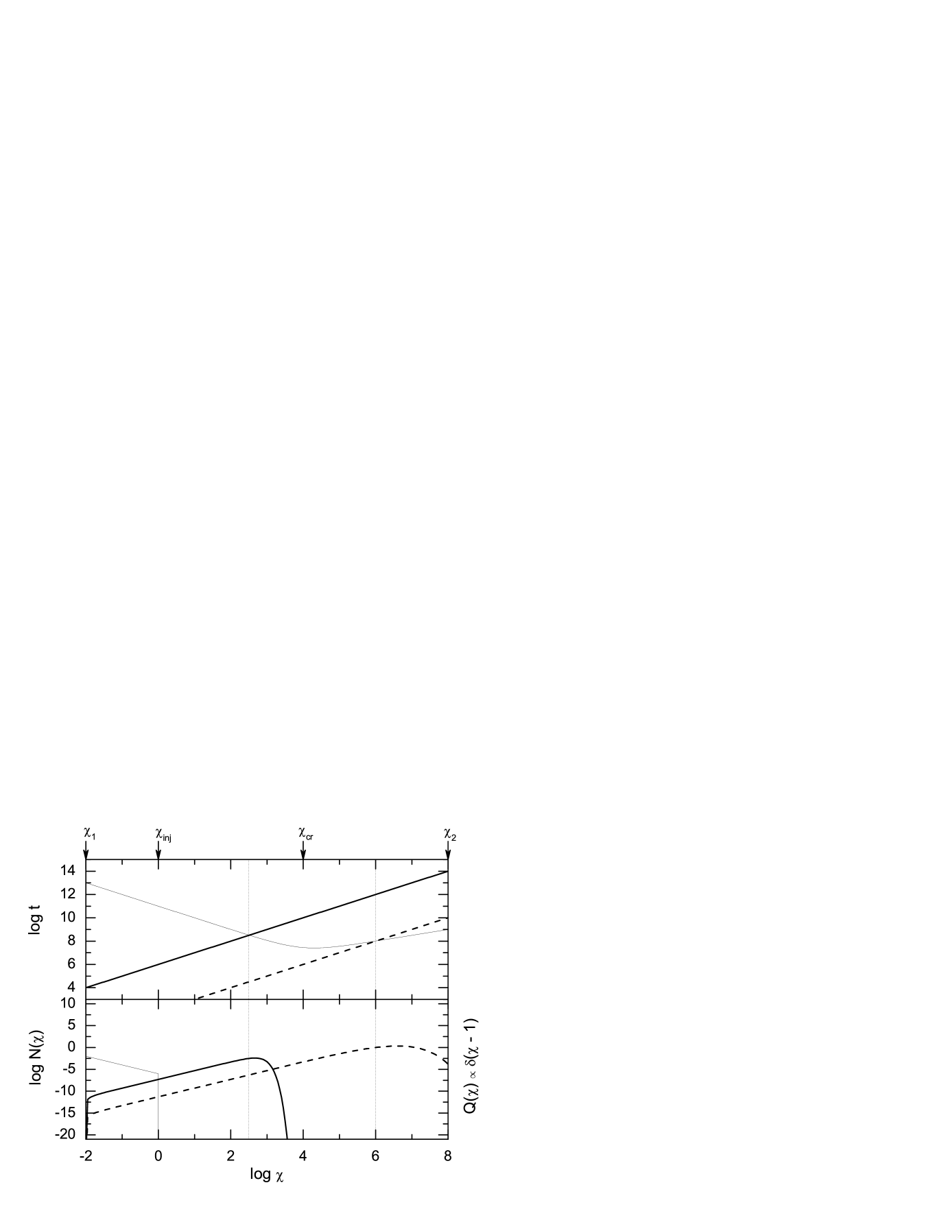
Figure 3: Upper panel: Stochastic acceleration timescales for fixed $q=1$ and different plasma parameters (thick solid and dashed lines). Thin solid line denotes inverse-Compton energy losses timescale considered with the assumed $\chi_{\rm cr}=10^{4}$. Lower panel: Particle spectra resulting from joint stochastic acceleration and inverse-Compton energy losses specified in the upper panel. The spectra correspond to the monoenergetic injection $Q(\chi)\propto\delta(\chi-1)$ with fixed $\int dp\,\widetilde{Q}(p)$, and no particle escape. Thin solid line denotes particle spectrum expected for the same injection and cooling conditions, but with the momentum diffusion effects neglected, $\widetilde{N}(\chi)$.

Figure 4: The same as Figure (3) except for $q=2$.

Let us consider first the case of a low-energy injection, such that $\chi_{\rm inj}<\min(\chi_{\rm Th},\,\chi_{\rm cr})$. The Green’s function (32) can be then approximated roughly by

$$\left.\mathcal{G}(\chi,\chi_{\rm inj})\right|_{\rm ic;\,\chi_{\rm inj}<}^{q\neq 1.5}\sim\left\{\begin{array}[]{ccc}{1\over 1+q}\,\chi_{1}^{-1-q}\,\chi^{2}\,e^{-\,{1\over 3-q}\,\left(\chi/\chi_{\rm Th}\right)^{3-q}}&{\rm for}&\chi<\chi_{\rm cr}\\ {1\over 1+q}\,\chi_{1}^{-1-q}\,e^{-\,{2\over\sqrt{\pi}}\,\Gamma(3-q)\,\Gamma(q-1.5)\,\left(\chi_{\rm cr}/\chi_{\rm Th}\right)^{3-q}}\,\chi^{2}\,e^{-\,{1\over 1.5-q}\,\left(\chi/\chi_{\rm KN}\right)^{1.5-q}}&{\rm for}&\chi>\chi_{\rm cr}\end{array}\right.\,.$$ (33)

For $\chi<\chi_{\rm cr}$ the Green’s function has the same form as the synchrotron case, which is expected in the Thomson regime. However, $\chi>\chi_{\rm cr}$, the KN effects modify the high-energy segment of the particle energy distribution. In particular, for $q<1.5$ (e.g. $q=1$ in Fig. 3) the spectrum is always of a ‘single-bump’ form, possessing either a sharp or a smooth exponential cut-off depending on whether we are in the Thomson or KN cooling regime, respectively. On the other hand, with $q>1.5$ (e.g. $q=2$ in Fig. 4) the acceleration and loss timescales can be equal at two different energies, in which case the particle spectra become concave, flattening smoothly from the exponential decrease $\propto\chi^{2}\,\exp\left[-{1\over 3-q}\left(\chi/\chi_{\rm Th}\right)^{3-q}\right]$ at $\chi_{\rm Th}<\chi<\chi_{\rm cr}$ to the asymptoticaly approached $\propto\chi^{2}$ continuum at $\chi>\chi_{\rm KN}$. Such spectra are shown in Figure (3-4) for $q=1$ and $q=2$, respectively, assuming monoenergetic injection with $\chi_{\rm inj}=1$, $\chi_{1}=10^{-2}$, $\chi_{\rm KN}=10^{4}$, and $\chi_{2}=10^{8}$. In each figure we use two different acceleration timescales (thick solid and dashed lines), but the radiative losses timescale, $t_{\rm loss}$, as well as the normalization of the injection function, $\int dp\,\widetilde{Q}(p)$, are kept constant. The emerging spectra are compared with the electron energy distribution $\widetilde{N}(\chi)$ corresponding to the same injection and cooling conditions, but with the momentum diffusion neglected (equations 29; thin solid lines in the lower panels of the figures).

In the case of $q\neq 1.5$ and high-energy injection $\chi_{\rm inj}>\chi_{\rm cr}$, the appropriate Green’s fuction retains again familiar shape $\left.\mathcal{G}(\chi,\chi_{\rm inj})\right|_{\rm ic;\,\chi_{\rm inj}>}^{q\neq 1.5}\sim{1\over 1+q}\,\chi_{1}^{-1-q}\,\chi^{2}\,e^{-\,{1\over 3-q}\,\left(\chi/\chi_{\rm T}\right)^{3-q}}$ at low particle momenta $\chi<\chi_{\rm cr}$. And again, at $\chi>\chi_{\rm cr}$ significant deviations from such a form may be observed, as follows from the approximate form of the Green’s function

$$\left.\mathcal{G}(\chi,\chi_{\rm inj})\right|_{\rm ic;\,\chi_{\rm inj}>}^{q\neq 1.5}\approx\chi^{2}\,e^{-{1\over 1.5-q}\left(\chi/\chi_{\rm KN}\right)^{1.5-q}}\,e^{-\,{2\over\sqrt{\pi}}\,\Gamma(3-q)\,\Gamma(q-1.5)\,\left(\chi_{\rm cr}/\chi_{\rm Th}\right)^{3-q}}\times$$ (34)

$$\times\int_{\chi_{1}}^{\min(\chi_{\rm inj},\chi)}d\chi^{\prime}\,\chi^{\prime-2-q}\,\exp\left\{{1\over 3-q}\left({\chi^{\prime}\over\chi_{\rm Th}}\right)^{3-q}\,F\!\left[{3\over 2},\,3-q,\,4-q,\,-{\chi^{\prime}\over\chi_{\rm cr}}\right]\right\}\quad{\rm for}\quad\chi>\chi_{\rm cr}$$

(see equation 32 with the $A^{-1}$ term neglected). The resulting particle spectra are plotted in Figures (5-6), where we consider two limiting cases of $q=1$ and $q=2$, and assume monoenergetic injection $Q(\chi)\propto\delta(\chi-\chi_{\rm inj})$ with $\chi_{\rm inj}=10^{7}$. All the other parameters are fixed as before. As shown, in addition to the spectral features discussed in the previous paragraph for the case of a low-energy injection (Figures 3-4), the radiatively-cooled continuum may be observed at high particles energies $\chi<\chi_{\rm inj}$, depending on the efficiency of the acceleration process. The KN effects manifest thereby by means of a characteristic spectral flattening over the ‘standard’ power-law form $\propto\chi^{-2}$, obviously only within the momentum range $\chi_{\rm cr}<\chi<\chi_{\rm inj}$, in agreement with the appropriate $\widetilde{N}(\chi)$ distribution (thin solid lines in the lower panels of Figures 5-6). Such a feature, being a direct result of a dominant IC/KN-regime radiative cooling with the momentum diffusion effects negligible, was discussed previously by, e.g., Kusunose & Takahara (2005); Moderski et al. (2005); Manolakou et al. (2007).

Figure 5: Upper panel: Stochastic acceleration timescales for fixed $q=1$ and different plasma parameters (thick solid and dashed lines). Thin solid line denotes inverse-Compton energy losses timescale considered with the assumed $\chi_{\rm cr}=10^{4}$. Lower panel: Particle spectra resulting from joint stochastic acceleration and inverse-Compton energy losses specified in the upper panel. The spectra correspond to the monoenergetic injection $Q(\chi)\propto\delta(\chi-10^{7})$ with fixed $\int dp\,\widetilde{Q}(p)$, and no particle escape. Thin solid line denotes particle spectrum expected for the same injection and cooling conditions, but with the momentum diffusion effects neglected, $\widetilde{N}(\chi)$.

Figure 6: The same as Figure (5) except for $q=2$.

Figure 7: Upper panel: Stochastic acceleration timescales for fixed $q=3/2$ and different plasma parameters (thick solid, dashed, and dotted lines). Thin solid line denotes inverse-Compton energy losses timescale considered with the assumed $\chi_{\rm cr}=10^{4}$. Lower panel: Particle spectra resulting from joint stochastic acceleration and inverse-Compton energy losses specified in the upper panel. The spectra correspond to the monoenergetic injection $Q(\chi)\propto\delta(\chi-1)$ with fixed $\int dp\,\widetilde{Q}(p)$, and no particle escape. Thin solid line denotes particle spectrum expected for the same injection and cooling conditions, but with the momentum diffusion effects neglected, $\widetilde{N}(\chi)$.

Finally, for completeness we note that with $q=1.5$ one can solve equation (23) to obtain

$$S(\chi)=\chi^{-2}\exp\left\{2\,\left({\chi_{\rm cr}\over\chi_{\rm T}}\right)^{3/2}\,\left({\rm ArcSinh}\!\sqrt{\chi/\chi_{\rm cr}}-{\sqrt{\chi/\chi_{\rm cr}}\over\sqrt{1+(\chi/\chi_{\rm cr})}}\right)\right\}\,.$$ (35)

This reduces to $S(\chi)\sim\chi^{-2}\,\exp\left[{2\over 3}\left(\chi/\chi_{\rm Th}\right)^{3/2}\right]$ for $\chi<\chi_{\rm cr}$, and can be approximated by $S(\chi)\sim 0.54\,\chi^{-1}\,\chi_{\rm cr}^{-1}$ for $\chi>\chi_{\rm cr}$. The resulting particle spectra, shown in Figure (7) for the case of a low-energy injection $Q(\chi)\propto\delta(\chi-1)$, are therefore $N(\chi<\chi_{\rm cr})\propto\chi^{2}\,\exp\left[-{2\over 3}\left(\chi/\chi_{\rm Th}\right)^{3/2}\right]$ at low momenta, or of the power-law form $N(\chi>\chi_{\rm cr})\propto\chi^{-\sigma^{\prime}}$ at higher momenta where the KN effects are important. Here $\sigma^{\prime}\equiv{t_{\rm acc}\over t_{\rm ic}(\chi>\chi_{\rm cr})}-2={\tau_{\rm acc}\over\tau_{\rm ic}}\,\chi_{\rm cr}^{1.5}-2$.

3.3 Bremsstrahlung and Coulomb Energy Losses

At high densities or low magnetic field (in general low Alfvén velocities) electron-electron and electron-ion interactions become important. These result in an elastic loss due to Coulomb collisions or radiative loss via bremsstrahlung. At low energies the bremsstrahlung loss rate is negligible when compared to the Coulomb loss rate, which is independent of energy for relativistic charge particles (see e.g. Petrosian, 1973, 2001). However, since the bremsstrahlung rate increases nearly linearly with energy, above some critical energy bremsstarahlung becomes dominant. The time scales associated with these processes approximately are

$$t_{\rm coul}=\tau_{\rm coul}\,\chi,\quad{\rm where}\quad\tau_{\rm coul}\equiv{p_{0}\over m_{\rm e}c}\,{2\over 3\,\sigma_{\rm Th}c\,n_{\rm g}\,\ln\Lambda}$$ (36)

and

$$t_{\rm brem}=\tau_{\rm brem}\,,\quad{\rm where}\quad\tau_{\rm brem}\equiv{\pi\over 3\,\alpha_{\rm fs}\sigma_{\rm Th}c\,n_{\rm g}}\,.$$ (37)

Here $n_{\rm g}$ is the background plasma density, the Coulomb logarithm $\ln\Lambda$ varies from 10 to 40 for variety of astrophysical plasma, $\alpha_{\rm fs}=1/137$ is the fine structure constant, and the bremsstrahlung rate includes electron-ion and electron-electron bramsstrahlung, and assumes completely unscreened limit with approximately $10\%$ (fully ionized) helium abundance (Blumenthal & Gould, 1970). The time scales are equal at energy $p_{\rm Coul}=\pi\,\ln\Lambda\,m_{\rm e}c/(2\,\alpha_{\rm fs})$. At higher energies the bremsstrahlung loss becomes unimportant compared to the synchrotron or IC losses. For example, the synchrotron loss becomes equal to and exceeds the bremsstrahlung loss at electron momenta $p\geq p_{\rm brem}\equiv(m_{e}/m_{p})(\alpha_{\rm fs}/\beta_{\rm A}^{2})\,m_{\rm e}c$ so that for bremsstrahlung to be at all important we need $1000<p/(m_{e}c)<10^{-5}\,\beta_{\rm A}^{-2}$, requiring $\beta_{\rm A}<0.003$. Below we investigate in some details stochastic acceleration for the conditions when the Coulomb and bremsstrahlung processes are the dominant loss processes.

At low energies, $p<p_{\rm Coul}$, Coulomb collision dominate. If $p_{0}\gg m_{e}c$ then in the range $m_{e}c\ll p\ll p_{\rm Coul}$ and for $q>1$, the appropriate Green’s function becomes

$$\left.\mathcal{G}(\chi,\chi_{\rm inj})\right|_{\rm coul}^{q>1}=\chi^{2}\,e^{{1\over 1-q}\,\left[\left({\chi_{1}\over\chi_{\rm eq}}\right)^{1-q}-\left({\chi\over\chi_{\rm eq}}\right)^{1-q}\right]}\,\left({1\over A}+\int^{\min[\chi_{\rm inj},\,\chi]}_{\chi_{1}}d\chi^{\prime}\,\chi^{\prime-(2+q)}\,e^{{1\over 1-q}\,\left[\left({\chi^{\prime}\over\chi_{\rm eq}}\right)^{1-q}-\left({\chi_{1}\over\chi_{\rm eq}}\right)^{1-q}\right]}\right)\approx$$

$$\approx\chi^{2}\,e^{-\,{1\over 1-q}\,\left({\chi\over\chi_{\rm eq}}\right)^{1-q}}\,{\chi_{\rm eq}^{-1-q}\,(-1)^{2/(1-q)}\over(1-q)^{2/(1-q)}}\,\Gamma\left[-{1+q\over 1-q}\,,\,-\,{\left(\min[\chi_{\rm inj},\,\chi]/\chi_{\rm eq}\right)^{1-q}\over 1-q},\,-\,{\left(\chi_{1}/\chi_{\rm eq}\right)^{1-q}\over 1-q}\right]$$ (38)

(see equations 22$-$23), where the equilibrium momentum $\chi_{\rm eq}=(\tau_{\rm coul}/\tau_{\rm acc})^{1/(1-q)}$ is defined by the $t_{\rm acc}=t_{\rm coul}$ condition, yielding $\vartheta_{\chi}=\chi_{\rm eq}^{q-1}/\chi$. Note that since $q>1$ are considered, the acceleration timescale is longer than the Coulomb interactions timescale for $\chi<\chi_{\rm eq}$. Thus, in the case of a low-energy particle injection with $\chi_{\rm inj}<\chi_{\rm eq}$, the emerging particle spectra are of the ‘cooled’ form $N(\chi)=\widetilde{N}(\chi)\propto const$ (see equation 29 with $\vartheta_{\chi}\propto\chi^{-1}$). If, however, higher-energy particles are injected to the system, an additional flat-spectrum component $N(\chi)\propto\chi^{2}$ is formed at $\chi>\chi_{\rm eq}$.

Let us finally note, that pure Coulomb energy losses and the Bohm limit $q=1$ correspond to the situation when $\vartheta_{\chi}=const$, and hence $S(\chi)=\chi^{-2+(\tau_{\rm acc}/\tau_{\rm coul})}$. The Green’s function (22) adopts then the form

$$\left.\mathcal{G}(\chi,\chi_{\rm inj})\right|_{\rm coul}^{q=1}=\chi^{2-{\tau_{\rm acc}\over\tau_{\rm coul}}}\,\left({1\over A}+\int^{\min[\chi_{\rm inj},\,\chi]}_{\chi_{1}}d\chi^{\prime}\,\chi^{\prime-4+{\tau_{\rm acc}\over\tau_{\rm coul}}}\right)\sim$$

$$\sim{1\over\sigma^{\prime}}\,\chi^{-\sigma^{\prime}}\,\left\{\begin{array}[]{ccc}\chi_{1}^{\sigma^{\prime}}&{\rm for}&\tau_{\rm acc}/\tau_{\rm coul}<2\\ \min^{\sigma^{\prime}}(\chi_{\rm inj},\,\chi)&{\rm for}&\tau_{\rm acc}/\tau_{\rm coul}>2\end{array}\right.\,,$$ (41)

where $\sigma^{\prime}\equiv{\tau_{\rm acc}\over\tau_{\rm coul}}-2$. Hence, if only $\tau_{\rm acc}<2\,\tau_{\rm coul}$, a power-law particle energy distribution $N(\chi)\propto\chi^{-\sigma^{\prime}}$ forms, with $-2<\sigma^{\prime}<0$. For any longer acceleration timescale, $\tau_{\rm acc}>2\,\tau_{\rm coul}$, and for the source function $Q(\chi)\propto\delta(\chi-\chi_{\rm inj})$, the emerging electron spectra are $N(\chi)\propto const$ for $\chi<\chi_{\rm inj}$, and $N(\chi)\propto\chi^{-\sigma^{\prime}}$ with $\sigma^{\prime}>0$ for $\chi>\chi_{\rm inj}$. This is consistent with the solution found by Bogdan & Schlickeiser (1985), who considered also synchrotron emission and finite escape timescale in addition to the Coulomb energy losses of ultrarelativistic electrons interacting with flat-spectrum turbulence $q=1$.

At higher energies and in the range $p_{\rm Coul}\ll p\ll p_{\rm brem}$ bremsstrahlung loss is the dominant process and the equilibrium momentum defined by the condition $t_{\rm acc}=t_{\rm brem}$ for $q<2$ becomes $\chi_{\rm eq}=(\tau_{\rm brem}/\tau_{\rm acc})^{1/(2-q)}$, yielding $\vartheta_{\chi}=\chi_{\rm eq}^{-(2-q)}$. Hence, the Green’s function (22) is

$$\left.\mathcal{G}(\chi,\chi_{\rm inj})\right|_{\rm brem}^{q<2}=\chi^{2}\,e^{-\,{1\over 2-q}\,\left({\chi\over\chi_{\rm eq}}\right)^{2-q}}\,\left({1\over A}+\int^{\min[\chi_{\rm inj},\,\chi]}_{\chi_{1}}d\chi^{\prime}\,\chi^{\prime-(2+q)}\,e^{{1\over 2-q}\,\left({\chi^{\prime}\over\chi_{\rm eq}}\right)^{2-q}}\right)\approx$$ (42)

$$\approx\chi^{2}\,e^{-\,{1\over 2-q}\,\left({\chi\over\chi_{\rm eq}}\right)^{2-q}}\,{\chi_{\rm eq}^{-1-q}\,(-1)^{3/(2-q)}\over(2-q)^{3/(2-q)}}\,\Gamma\left[-{1+q\over 2-q}\,,\,-\,{\left(\min[\chi_{\rm inj},\,\chi]/\chi_{\rm eq}\right)^{2-q}\over 2-q},\,-\,{\left(\chi_{1}/\chi_{\rm eq}\right)^{2-q}\over 2-q}\right]$$

(equations 22$-$23). In other words, for any injection conditions the expected electron energy distribution is of the $N(\chi)\propto\chi^{2}\,\exp\left[-{1\over 2-q}\left(\chi/\chi_{\rm eq}\right)^{2-q}\right]$ form, except for the case when high energy particles with $\chi_{\rm inj}>\chi_{\rm eq}$ are injected to the system. Such high energy particles subjected to the bremsstrahlung energy losses form then an additional ‘cooled’ high-energy power-law tail $N(\chi)\propto\chi^{-1}$ in the momentum range between $\chi_{\rm eq}$ and $\chi_{\rm inj}$, in agreement with the appropriate form of $\widetilde{N}(\chi)$ with $\vartheta_{\chi}=const$ (see equation 29).

The situation changes for $q=2$, since both the acceleration and cooling timescales are now independent of electrons’ energy. In this case $S(\chi)=\chi^{-2+(\tau_{\rm acc}/\tau_{\rm brem})}$, and the Green’s function (22) adopts the form

$$\left.\mathcal{G}(\chi,\chi_{\rm inj})\right|_{\rm brem}^{q=2}=\chi^{2-{\tau_{\rm acc}\over\tau_{\rm brem}}}\,\left({1\over A}+\int^{\min[\chi_{\rm inj},\,\chi]}_{\chi_{1}}d\chi^{\prime}\,\chi^{\prime-4+{\tau_{\rm acc}\over\tau_{\rm brem}}}\right)\sim$$

$$\sim{1\over 1-\sigma^{\prime}}\,\chi^{-\sigma^{\prime}}\,\left\{\begin{array}[]{ccc}\chi_{1}^{-1+\sigma^{\prime}}&{\rm for}&\tau_{\rm acc}/\tau_{\rm brem}<3\\ \min^{-1+\sigma^{\prime}}(\chi_{\rm inj},\,\chi)&{\rm for}&\tau_{\rm acc}/\tau_{\rm brem}>3\end{array}\right.\,,$$ (45)

where $\sigma^{\prime}\equiv{\tau_{\rm acc}\over\tau_{\rm brem}}-2$. This is consistent with the appropriate Green’s function found by Schlickeiser et al. (1987) who, in a framework of the ‘hard-sphere’ approximation $q=2$, considered also synchrotron emission and particle escape in addition to the bremsstrahlung radiation. The solution (45) implies that within the whole energy range the expected electron energy distribution is of the power-law form $N(\chi)\propto\chi^{-\sigma^{\prime}}$, with the power-law index $-2<\sigma^{\prime}<1$. For any longer acceleration timescale, $\tau_{\rm acc}>3\,\tau_{\rm brem}$, and monoenergetic injection $Q(\chi)\propto\delta(\chi-\chi_{\rm inj})$, the emerging electron spectra are expected to be of the $N(\chi)\propto\chi^{-1}$ form for $\chi<\chi_{\rm inj}$, while $N(\chi)\propto\chi^{-\sigma^{\prime}}$ with $\sigma^{\prime}>1$ for $\chi>\chi_{\rm inj}$.

4 Efficient Particle Escape

In this section we investigate steady-state solutions to the momentum diffusion equation of radiating ultrarelativistic particles with a finite escape timescale (equation 6). Our analytical approach force us to consider only the limiting cases of turbulent spectral indices $q=2$ or $q=1$, as well as to restrict the analysis of radiative losses to the synchrotron and/or IC-Thompson regime processes, ($\vartheta_{\chi}\propto\chi$). We note that the global approximation to the solution of the momentum diffusion equation not necessarily restricted to some particular values of the $q$ parameter, with the regular energy losses and particle escape terms included, were studied by Gallegos-Cruz & Perez-Peraza (1995) by using the WKBJ method. Just us before, we consider finite energy range of particles undergoing momentum diffusion, $0<\chi_{1},\,\chi_{2}<\infty$, strictly related to the finite wavelength range of interacting turbulent modes. We construct the Green’s function accordingly to the procedure outlined in the previous section § 3, with addition of the escape term ($\varepsilon\neq 0$) and with a different boundary conditions. Specifically, we change equation (5) to

$${\partial\mathcal{N}\over\partial\tau}+\left.\mathcal{F}\right|_{\chi_{2}}-\left.\mathcal{F}\right|_{\chi_{1}}=\int_{\chi_{1}}^{\chi_{2}}d\chi\,Q(\chi,\tau)-\varepsilon\,\int_{\chi_{1}}^{\chi_{2}}d\chi\,\chi^{2-q}\,N(\chi)\,,$$ (46)

where the particle flux in the momentum space $\mathcal{F}[N(\chi)]$ is defined in the same way as previously (equation 19). As evident, the no-flux boundary conditions, $\mathcal{F}[N(\chi_{1})]=\mathcal{F}[N(\chi_{2})]=0$, and conservation of total number of particles, $\partial\mathcal{N}/\partial\tau=0$, (within the energy range $[\chi_{1},\chi_{2}]$) implies that the particle injection is completely balanced by the particle escape. We will assume this to be the case in this section. Physical realization of these would imply presence of an another efficient yet unspecified acceleration process operating at $\chi<\chi_{1}$, which prevent negative particle momentum flux through the $\chi_{1}$ boundary. As shown below, the solutions we obtain agree with the ones discussed in the literature for singular boundary conditions for the infinite momentum range (Jones, 1970; Schlickeiser, 1984; Bogdan & Schlickeiser, 1985; Park & Petrosian, 1995), as long as we are dealing with particle momenta $\chi\gg\chi_{1}$ and $\chi\ll\chi_{2}$.

4.1 ‘Hard-Sphere’ Approximation

‘Hard-Sphere’ approximation for the momentum diffusion of ultrarelativistic electrons undergoing synchrotron energy losses corresponds to the fixed $q=2$ and $\vartheta_{\chi}=\chi/\chi_{\rm eq}$ (see equations 4 and 24). With these, the equation (6) adopts the form

$$\chi^{2}\,N^{\prime\prime}(\chi)+\chi_{\rm eq}^{-1}\,\chi^{2}\,N^{\prime}(\chi)+\left(2\,\chi_{\rm eq}^{-1}\,\chi-2-\varepsilon\right)\,N(\chi)=-Q(\chi)\,.$$ (47)

The two linearly-independent particular solutions to the homogeneous form of the above equation are

$$y_{1}(\chi) = \chi^{\sigma+1}\,e^{-{\chi\over\chi_{\rm eq}}}\,U\!\left[\sigma-1,\,2\sigma+2,\,{\chi\over\chi_{\rm eq}}\right]\,,$$

$$y_{2}(\chi) = \chi^{\sigma+1}\,e^{-{\chi\over\chi_{\rm eq}}}\,M\!\left[\sigma-1,\,2\sigma+2,\,{\chi\over\chi_{\rm eq}}\right]\,,$$ (48)

where $U[a,b,z]$ and $M[a,b,z]$ are Tricomi and Kummer confluent hypergeometrical functions, respectively, and $\sigma\equiv-(1/2)+[(9/4)+\varepsilon]^{1/2}$. Introducing next their linear combinations, $u_{1}(\chi)=y_{1}(\chi)+\alpha\,y_{2}(\chi)$ and $u_{2}(\chi)=y_{1}(\chi)+\beta\,y_{2}(\chi)$, one may find that the no-flux boundary conditions $\mathcal{F}[u_{1}(\chi_{1})]=\mathcal{F}[u_{2}(\chi_{2})]=0$ are fulfilled for

$$\alpha=(2+\sigma)\,{U\!\left[\sigma,\,2\sigma+2,\,\chi_{1}/\chi_{\rm eq}\right]\over M\!\left[\sigma,\,2\sigma+2,\,\chi_{1}/\chi_{\rm eq}\right]}\,,\quad{\rm and}\quad\beta=(2+\sigma)\,{U\!\left[\sigma,\,2\sigma+2,\,\chi_{2}/\chi_{\rm eq}\right]\over M\!\left[\sigma,\,2\sigma+2,\,\chi_{2}/\chi_{\rm eq}\right]}\,.$$ (49)

This gives the Green’s function of the problem as

$$\left.\mathcal{G}(\chi,\chi_{\rm inj})\right|_{\rm esc}^{q=2}={\Gamma(\sigma-1)\over\Gamma(2\sigma+2)}\,\left(\alpha-\beta\right)^{-1}\,\chi_{\rm inj}^{-2}\,\chi_{\rm eq}^{-2\sigma-1}\,e^{\chi_{\rm inj}/\chi_{\rm eq}}\times$$

$$\times\quad\left\{\begin{array}[]{ccc}\left[y_{1}(\chi)+\alpha\,y_{2}(\chi)\right]\,\left[y_{1}(\chi_{\rm inj})+\beta\,y_{2}(\chi_{\rm inj})\right]&{\rm for}&\chi_{1}\leq\chi<\chi_{\rm inj}\\ \left[y_{1}(\chi_{\rm inj})+\alpha\,y_{2}(\chi_{\rm inj})\right]\,\left[y_{1}(\chi)+\beta\,y_{2}(\chi)\right]&{\rm for}&\chi_{\rm inj}<\chi\leq\chi_{2}\end{array}\right.\,.$$ (52)

Figure 8: ‘Hard-sphere approximation’ ($q=2$): particle spectra resulting from joint stochastic acceleration, particle escape, and synchrotron energy losses. The spectra correspond to the monoenergetic injection $Q(\chi)\propto\delta(\chi-\chi_{\rm inj})$ with fixed normalization, fixed acceleration and cooling rates, but different escape timescales (parameter $\varepsilon=3$, $0.1$, $10^{-4}$; dotted, dashed, and solid lines, respectively). For illustration, $\chi_{1}=10^{-2}$, $\chi_{\rm inj}=1$, $\chi_{\rm eq}=10^{6}$, and $\chi_{2}=10^{8}$ have been selected.

Figure 9: The same as FIgure (8) except for $\chi_{\rm inj}=10^{6}$.

In order to investigate the above solution, let us consider first the case $\chi_{1}\ll\chi_{\rm inj}\ll\chi_{\rm eq}\ll\chi_{2}$, and use the standard expansion of the confluent hypergeometrical functions: $U[a,b,z]\sim z^{-a}$ and $M[a,b,z]\sim\Gamma(b)\,e^{z}\,z^{a-b}/\Gamma(a)$ for $z\rightarrow\infty$, while $U[a,b,z]\sim\Gamma(b-1)\,z^{1-b}/\Gamma(a)$ and $M[a,b,z]\sim 1$ for $z\rightarrow 0$ (Abramowitz & Stegun, 1964). In this limit one gets

$$\left.\mathcal{G}(\chi,\chi_{\rm inj})\right|_{\rm esc,\,\chi_{\rm inj}<}^{q=2}\sim\left\{\begin{array}[]{ccc}{1\over 2\sigma+1}\,\chi_{\rm inj}^{-\sigma-2}\,\chi^{\sigma+1}&{\rm for}&\chi_{1}<\chi<\chi_{\rm inj}\\ {1\over 2\sigma+1}\,\chi_{\rm inj}^{\sigma-1}\,\chi^{-\sigma}&{\rm for}&\chi_{\rm inj}<\chi\ll\chi_{\rm eq}\\ {\Gamma(\sigma-1)\over\Gamma(2\sigma+2)}\,\chi_{\rm inj}^{\sigma-1}\,\chi_{\rm eq}^{-\sigma-2}\,\chi^{2}\,e^{-\chi/\chi_{\rm eq}}&{\rm for}&\chi_{\rm eq}\lesssim\chi<\chi_{2}\end{array}\right.\,.$$ (53)

Thus, by moving the critical momenta $\chi_{1}$ and $\chi_{2}$ toward $0$ and $\infty$, respectively, the resultant Green’s function approaches asymptotically — as expected — the corresponding Green’s function for singular boundary conditions obtained by Jones (1970); Schlickeiser (1984) and Park & Petrosian (1995). In particular, one can find that with the monoenergetic injection $Q(\chi)\propto\delta(\chi-\chi_{\rm inj})$, the resulting electron energy distribution is then of the form $N(\chi<\chi_{\rm inj})\propto\chi^{\sigma+1}$ and $N(\chi>\chi_{\rm inj})\propto\chi^{-\sigma}$ up to maximum momentum $\chi_{\rm eq}$. Moreover, for the increasing escape timescale $\varepsilon\rightarrow 0$, one has $\sigma\approx 1$ and the pile-up bump $N(\chi)\propto\chi^{2}\,\exp\left[-\chi/\chi_{\rm eq}\right]$ emerging around $\chi\sim\chi_{\rm eq}$ energies. This is shown in Figure (8), where we fixed normalization of the monoenergetic injection $\int dp\,\widetilde{Q}(p)$, acceleration and losses timescales, but varied the escape timescale ($\varepsilon=3$, $0.1$, $10^{-4}$; dotted, dashed, and solid lines, respectively). For illustration we have selected $\chi_{1}=10^{-2}$, $\chi_{\rm inj}=1$, $\chi_{\rm eq}=10^{6}$, and $\chi_{2}=10^{8}$.

When high energy particles are injected to the system, such that $\chi_{1}\ll\chi_{\rm eq}\ll\chi_{\rm inj}\ll\chi_{2}$, one may find useful asymptotic expansion of the Green’s function

$$\left.\mathcal{G}(\chi,\chi_{\rm inj})\right|_{\rm esc,\,\chi_{\rm inj}>}^{q=2}\sim\left\{\begin{array}[]{ccc}{\Gamma(\sigma-1)\over\Gamma(2\sigma+2)}\,\chi_{\rm eq}^{-\sigma-2}\,\chi^{\sigma+1}\,e^{-\chi/\chi_{\rm eq}}&{\rm for}&\chi_{1}<\chi\lesssim\chi_{\rm eq}\\ \chi^{-2}\,\chi_{\rm eq}&{\rm for}&\chi_{\rm eq}\ll\chi<\chi_{\rm inj}\\ \chi_{\rm inj}^{-4}\,\chi_{\rm eq}\,e^{\chi_{\rm inj}/\chi_{\rm eq}}\,\chi^{2}\,e^{-\chi/\chi_{\rm eq}}&{\rm for}&\chi_{\rm inj}<\chi<\chi_{2}\end{array}\right.\,.$$ (54)

That is, for the monoenergetic injection $Q(\chi)\propto\delta(\chi-\chi_{\rm inj})$ with $\chi_{\rm inj}>\chi_{\rm eq}$ the resulting electron energy distribution is of the form $N(\chi)\propto\chi^{\sigma+1}\,\exp\left[-\chi/\chi_{\rm eq}\right]$ for $\chi\lesssim\chi_{\rm eq}$. However, within the energy range $\chi_{\rm eq}<\chi<\chi_{\rm inj}$ the power-law tail $N(\chi)\propto\chi^{-2}$ emerges, representing radiatively ($\vartheta_{\chi}\propto\chi$) cooled high-energy particles injected to the system, undergoing negligible (when compared to the energy loss rate) momentum diffusion. At even higher energies, $\chi>\chi_{\rm inj}$, the particle spectrum cuts-off rapidly. This is shown in Figure (9), where, as before, we fixed normalization of the monoenergetic injection $\int dp\,\widetilde{Q}(p)$, acceleration and losses timescales, but varied the escape timescale ($\varepsilon=3$, $0.1$, $10^{-4}$; dotted, dashed, and solid lines, respectively). For illustration we have selected $\chi_{1}=10^{-2}$, $\chi_{\rm eq}=10^{2}$, $\chi_{\rm inj}=10^{6}$, and $\chi_{2}=10^{8}$. Note, that the esape timescale, and hence parameter $\varepsilon$, influences now the slope and normalization of particle energy distribution only in the ‘low-energy’ regime $\chi<\chi_{\rm eq}$, such that the spectrum approaches $\propto x^{2}$ for $\varepsilon\rightarrow 0$.

4.2 Bohm Limit

Bohm limit for the momentum diffusion of ultrarelativistic electrons undergoing synchrotron energy losses corresponds to $q=1$ and $\vartheta_{\chi}=\chi/\chi_{\rm eq}^{2}$ (see equations 4 and 24). The difference with the ‘hard-sphere’ approximation is that the balance between acceleration and escape timescales, $t_{\rm acc}=t_{\rm esc}$, define now yet another critical energy, $\chi_{\rm esc}=\varepsilon^{-1/2}$ and equation (6) takes the form

$$\chi\,N^{\prime\prime}(\chi)+\left(\chi_{\rm eq}^{-2}\,\chi^{2}-1\right)\,N^{\prime}(\chi)+\left(2\,\chi_{\rm eq}^{-2}\,\chi-\chi_{\rm esc}^{-2}\,\chi\right)\,N(\chi)=-Q(\chi)\,.$$ (55)

The two linearly-independent particular solutions to the homogeneous form of the above equation are

$$y_{1}(\chi) = \chi^{2}\,e^{-{1\over 2}\,\left({\chi\over\chi_{\rm eq}}\right)^{2}}\,U\!\left[\eta,\,2,\,{1\over 2}\left({\chi\over\chi_{\rm eq}}\right)^{2}\right]\,,$$

$$y_{2}(\chi) = \chi^{2}\,e^{-{1\over 2}\,\left({\chi\over\chi_{\rm eq}}\right)^{2}}\,M\!\left[\eta,\,2,\,{1\over 2}\left({\chi\over\chi_{\rm eq}}\right)^{2}\right]\,,$$ (56)

where $\eta\equiv{1\over 2}(\chi_{\rm eq}/\chi_{\rm esc})^{2}$. Defining $u_{1}(\chi)=y_{1}(\chi)+\alpha\,y_{2}(\chi)$ and $u_{2}(\chi)=y_{1}(\chi)+\beta\,y_{2}(\chi)$, one finds that the no-flux boundary conditions $\mathcal{F}[u_{1}(\chi_{1})]=\mathcal{F}[u_{2}(\chi_{2})]=0$ corresponds to

$$\alpha=2\,{U\!\left[\eta+1,\,3,\,{1\over 2}\left(\chi_{1}/\chi_{\rm eq}\right)^{2}\right]\over M\!\left[\eta+1,\,3,\,{1\over 2}\left(\chi_{1}/\chi_{\rm eq}\right)^{2}\right]}\,,\quad{\rm and}\quad\beta=2\,{U\!\left[\eta+1,\,3,\,{1\over 2}\left(\chi_{2}/\chi_{\rm eq}\right)^{2}\right]\over M\!\left[\eta+1,\,3,\,{1\over 2}\left(\chi_{2}/\chi_{\rm eq}\right)^{2}\right]}\,.$$ (57)

This gives the Green’s function of the problem as

$$\left.\mathcal{G}(\chi,\chi_{\rm inj})\right|_{\rm esc}^{q=1}={1\over 4}\,\Gamma(\eta)\,\left(\alpha-\beta\right)^{-1}\,\chi_{\rm inj}^{-2}\,\chi_{\rm eq}^{-2}\,e^{{1\over 2}(\chi_{\rm inj}/\chi_{\rm eq})^{2}}\times$$

$$\times\quad\left\{\begin{array}[]{ccc}\left[y_{1}(\chi)+\alpha\,y_{2}(\chi)\right]\,\left[y_{1}(\chi_{\rm inj})+\beta\,y_{2}(\chi_{\rm inj})\right]&{\rm for}&\chi_{1}\leq\chi<\chi_{\rm inj}\\ \left[y_{1}(\chi_{\rm inj})+\alpha\,y_{2}(\chi_{\rm inj})\right]\,\left[y_{1}(\chi)+\beta\,y_{2}(\chi)\right]&{\rm for}&\chi_{\rm inj}<\chi\leq\chi_{2}\end{array}\right.\,.$$ (60)

Let us consider first the case $\chi_{1}\ll\chi_{\rm inj}\ll\chi_{\rm eq}\ll\chi_{2}$ for which he Green’s function of equation (60) can be then approximated as

$$\left.\mathcal{G}(\chi,\chi_{\rm inj})\right|_{\rm esc,\,\chi_{\rm inj}<}^{q=1}\sim\left\{\begin{array}[]{ccc}{1\over 2}\,\chi_{\rm inj}^{-2}\,\chi^{2}&{\rm for}&\chi_{1}<\chi<\chi_{\rm inj}\\ {1\over 2}&{\rm for}&\chi_{\rm inj}<\chi\ll\chi_{\rm eq}\\ 2^{\eta-2}\,\Gamma(\eta)\,\chi_{\rm eq}^{-2+2\,\eta}\,\chi^{2-2\,\eta}\,e^{-{1\over 2}(\chi/\chi_{\rm eq})^{2}}&{\rm for}&\chi_{\rm eq}\lesssim\chi<\chi_{2}\end{array}\right.\,.$$ (61)

Note that, as expected, in the limits $\chi_{1}\rightarrow 0$ and $\chi_{2}\rightarrow\infty$, the Green’s function (60) approaches asymptotically the solution obtained for singular boundary conditions by Bogdan & Schlickeiser (1985). As shown in Figure (10), for a monoenergetic injection $Q(\chi)\propto\delta(\chi-\chi_{\rm inj})$, the resulting electron energy distribution is $N(\chi<\chi_{\rm inj})\propto\chi^{2}$ and $N(\chi>\chi_{\rm inj})\propto const$ up to maximum momentum $\chi_{\rm eq}$, with the spectral indexes independent of the value of the escape timescale. However, for energies near and above $\chi_{\rm eq}$ the spectra depend on the value of $\eta$. For $\eta\rightarrow 0$, ı.e. when the escape timescale is large, the familiar bump $N(\chi)\propto\chi^{2}\,\exp\left[-{1\over 2}(\chi/\chi_{\rm eq})^{2}\right]$ emerges around $\chi\sim\chi_{\rm eq}$ energies (solid line). In the opposite case, when $\eta>1$ (or $\chi_{\rm eq}>\chi_{\rm esc}$), no pile-up bump is present, and the electron spectrum cut-offs exponentially at $\chi_{\rm esc}$ momenta (dashed and dotted lines). Here, as before, we fixed the normalization of the monoenergetic injection $\int\widetilde{Q}(p)\,dp$, and the acceleration and loss timescales, but varied the escape timescale such that $\chi_{\rm esc}=10^{5}$, $10^{6}$, and $10^{7}$ (dotted, dashed, and solid lines, respectively). We choose $\chi_{1}=10^{-2}$, $\chi_{\rm inj}=1$, $\chi_{\rm eq}=10^{6}$, and $\chi_{2}=10^{8}$.

Figure 10: Bohm Limit ($q=1$): particle spectra resulting from joint stochastic acceleration, particle escape, and synchrotron energy losses. The spectra correspond to the monoenergetic injection $Q(\chi)\propto\delta(\chi-\chi_{\rm inj})$ with fixed normalization, fixed acceleration and cooling rates, but different escape timescales (critical momenta $\chi_{\rm esc}=10^{5}$, $10^{6}$, $10^{7}$; dotted, dashed, and solid lines, respectively). For illustration, $\chi_{1}=10^{-2}$, $\chi_{\rm inj}=1$, $\chi_{\rm eq}=10^{6}$, and $\chi_{2}=10^{8}$ have been selected.

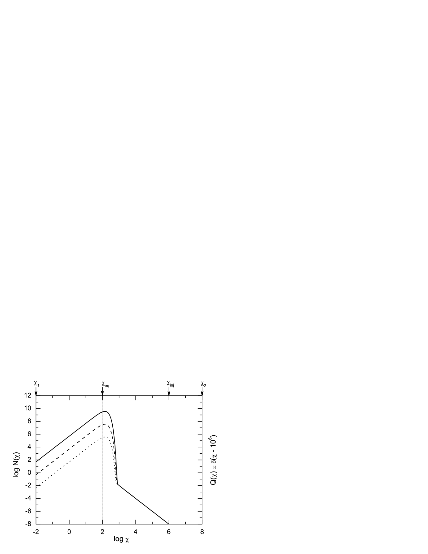
Figure 11: The same as Figure (10) except for $\chi_{\rm inj}=10^{6}$.

In the case when $\chi_{1}\ll\chi_{\rm eq}\ll\chi_{\rm inj}\ll\chi_{2}$ the asymptotic expansion of the Green’s function (60) yields

$$\left.\mathcal{G}(\chi,\chi_{\rm inj})\right|_{\rm esc,\,\chi_{\rm inj}>}^{q=1}\sim\left\{\begin{array}[]{ccc}2^{\eta-2}\,\Gamma(\eta)\,\chi_{\rm inj}^{-2\eta}\,\chi_{\rm eq}^{2\eta-2}\,\chi^{2}\,e^{-{1\over 2}\,(\chi/\chi_{\rm eq})^{2}}&{\rm for}&\chi_{1}<\chi\lesssim\chi_{\rm eq}\\ \chi_{\rm inj}^{-2\eta}\,\chi_{\rm eq}^{2}\,\chi^{2\eta-2}&{\rm for}&\chi_{\rm eq}\ll\chi<\chi_{\rm inj}\\ \chi_{\rm inj}^{2\eta-4}\,\chi_{\rm eq}^{2}\,\chi^{2\eta-2}\,e^{{1\over 2}\,(\chi_{\rm inj}/\chi_{\rm eq})^{2}}\,e^{-{1\over 2}\,(\chi/\chi_{\rm eq})^{2}}&{\rm for}&\chi_{\rm inj}\lesssim\chi<\chi_{2}\end{array}\right.\,.$$ (62)

Again as above, the spectrum is different in the case of high energy injection. For example, as shown in Figure (11), for the monoenergetic injection $Q(\chi)\propto\delta(\chi-\chi_{\rm inj})$ with $\chi_{\rm inj}>\chi_{\rm eq}$ the resulting electron energy distribution is of the form $N(\chi)\propto\chi^{2}\,\exp\left[-{1\over 2}(\chi/\chi_{\rm eq})^{2}\right]$ for $\chi\lesssim\chi_{\rm eq}$, while $N(\chi)\propto\chi^{2\eta-2}$ for $\chi_{\rm eq}\ll\chi<\chi_{\rm inj}$. It is interesting to note that the Bohm limit case behaves differently from the $q=2$ case and analogous injection condition. The escape timescale affecs now (via the parameter $\chi_{\rm esc}$, or $\eta$) the normalization of the low-energy ($\chi<\chi_{\rm eq}$) segment of the particle spectrum but not its power-law slope. It determines, on the other hand, the ‘radiatively-cooled’ part of the particle distribution in the range $\chi_{\rm eq}<\chi<\chi_{\rm inj}$, which is, however, very close to the standard $\propto\chi^{-2}$ for any $\chi_{\rm esc}\gg\chi_{\rm eq}$ (or $\eta\ll 1$). Here, as before, we fixed normalization of the monoenergetic injection $\int dp\,\widetilde{Q}(p)$, and the acceleration and loss timescales, but varied the escape timescale such that $\chi_{\rm esc}=10^{5}$, $10^{6}$, and $10^{7}$ (dotted, dashed, and solid lines, respectively). Also we set $\chi_{1}=10^{-2}$, $\chi_{\rm inj}=1$, $\chi_{\rm eq}=10^{6}$, and $\chi_{2}=10^{8}$.

5 Emission Spectra

In the previous sections § 3 and § 4, we showed that stochastic interactions of radiating ultrarelativistic electrons (Lorentz factors $\gamma\equiv p/m_{\rm e}c\gg 1$) with turbulence characterized by a power-law spectrum $\mathcal{W}(k)\propto k^{-q}$ result in formation of a ‘universal’ high-energy electron energy distribution

$$n_{\rm e}(\gamma)=n_{0}\,\gamma^{2}\,\exp\left[-{1\over a}\,\left({\gamma\over\gamma_{\rm eq}}\right)^{a}\right]\,,$$ (63)

as long as particle escape from the system is inefficient and the radiative cooling rate scales with some power of electron energy. Here the equilibrium energy $\gamma_{\rm eq}$ is defined by the balance between acceleration and the energy losses timescales, while the parameter $a$ depends on the dominant radiative cooling process and the turbulence spectrum. In particular, for either synchrotron or IC/Thomson-regime cooling one has $a=3-q$. In the case of dominant IC/KN-regime energy losses (with $q<1.5$) one has instead $a=1.5-q$. Below we investigate in more details emission spectra resulting from such an electron distribution.

5.1 Synchrotron Emission

Assuming isotropic distribution of momenta of radiating electrons with energy spectrum $n_{\rm e}(\gamma)$, the synchrotron emissivity can be found as

$$j_{\rm\nu,\,syn}(\nu)={\sqrt{3}\,e^{3}B\over 4\pi\,m_{\rm e}c^{2}}\int\,d\gamma\,\mathcal{R}\!\left({\nu\over\nu_{c}\,\gamma^{2}}\right)\,n_{\rm e}(\gamma)\,$$ (64)

where $\nu_{c}=3eB/4\pi m_{\rm e}c$,

$$\mathcal{R}(x)={x^{2}\over 2}\,K_{4/3}\left({x\over 2}\right)\,K_{1/3}\left({x\over 2}\right)-0.3\,{x^{3}\over 2}\,\left[K_{4/3}^{2}\left({x\over 2}\right)-K_{1/3}^{2}\left({x\over 2}\right)\right]\,,$$ (65)

and $K_{\mu}\left(z\right)$ is a modified Bessel function of the second order (Crusius & Schlickeiser, 1986). Relatively complicated function (65) can be instead conveniently approximated by $\mathcal{R}(x)\approx 1.81\times\left(1.33+x^{-2/3}\right)^{-1/2}e^{-x}$ (Zirakashvili & Aharonian, 2007), allowing for some analytical investigation of the integral (64). In particular, one may find that the synchrotron emissivity in a frequency range $\nu<\nu_{\rm syn}\equiv\nu_{c}\,\gamma_{\rm eq}^{2}$ is of the form $j_{\rm\nu,\,syn}(\nu<\nu_{\rm syn})\propto\nu^{1/3}$, as expected in the case of a very hard (inverted) electron energy distribution at low energies, $n_{\rm e}(\gamma<\gamma_{\rm eq})\propto\gamma^{2}$. At higher frequencies, however, the synchrotron spectrum steepens. In order to evaluate such a high-frequency spectral component, we use the introduced approximation for $\mathcal{R}(x)$, electron spectrum as given in (63), and with these we re-write synchrotron emissivity (64) as

$$j_{\rm\nu,\,syn}(\nu)\approx{1.81\,\sqrt{3}\,e^{3}B\,\gamma_{\rm eq}^{3}n_{0}\over 4\pi\,m_{\rm e}c^{2}}\int\,dy\,g(\omega,y)\,\exp\left[-\omega\,h(\omega,y)\right]\,,$$ (66)

where $\omega\equiv\nu/\nu_{\rm syn}$, $y\equiv\gamma/\gamma_{\rm eq}$, $g(\omega,y)\equiv y^{2}\,(1.33+\omega^{-2/3}y^{4/3})^{-1/2}$, and $h(\omega,y)\equiv y^{-2}+y^{a}/(\omega\,a)$.

Figure 12: Synchrotron spectra resulting from the electron energy distribution (63) for fixed parameters $B$, $n_{0}$, and $\gamma_{\rm eq}$. Solid lines correspond to integration of the exact form of $\mathcal{R}(x)$ as given in equation (65), while dashed lines to the approximate formulae following from (67). Different cases for the parameter $a$ are considered in the plot, namely (a) $a=3-q$ with $q=1$, (b) $a=3-q$ with $q=2$, and (c) $a=1.5-q$ with $q=1$.

With such a form it can be noted that for large $\omega$, i.e. for $\nu>\nu_{\rm syn}$, the integral of interest can be perform approximately using the steepest descent method (see Petrosian, 1981). This gives

$$j_{\rm\nu,\,syn}(\nu>\nu_{\rm syn})\simeq{1.81\,\sqrt{3}\,e^{3}B\,\gamma_{\rm eq}^{3}n_{0}\over 4\pi\,m_{\rm e}c^{2}}\,\sqrt{{2\pi\over\omega\,h^{\prime\prime}(\omega,y_{\star})}}\,\,g(\omega,y_{\star})\,\exp\left[-\omega\,h(\omega,y_{\star})\right]\simeq$$

$$\simeq{0.54\,e^{3}B\,\gamma_{\rm eq}^{3}n_{0}\over m_{\rm e}c^{2}\,\sqrt{2+a}}\,\left({2\nu\over\nu_{\rm syn}}\right)^{{6-a\over 4+2a}}\,\left[1+\left({2\nu\over\nu_{\rm syn}}\right)^{-{2a\over 6+3a}}\right]^{-1/2}\,\exp\left[-{2+a\over 2a}\,\left({2\nu\over\nu_{\rm syn}}\right)^{{a\over 2+a}}\right]\,,$$ (67)

where $y_{\star}=(2\omega)^{1/(2+a)}$ is a global maximum of $h(\omega,y)$, and $h^{\prime\prime}(\omega,y)=\partial^{2}h(\omega,y)/\partial y^{2}$. Thus, the high-energy synchrotron component drops much less rapidly than suggested by the emissivity of a single electron, $\mathcal{R}(x)\propto e^{-x}$. For example, assuming synchrotron (and/or IC/Thompson-regime) dominance $a=3-q$, the synchrotron emissivity reads very roughly as

$$j_{\rm\nu,\,syn}\left(\nu>\nu_{\rm syn}\right)\propto\nu^{1/2}\,\exp\left[-1.4\,\left(\nu/\nu_{\rm syn}\right)^{1/2}\right]\,\,\,\,\,{\rm for}\,\,\,\,\,q=1,$$ (68)

or

$$j_{\rm\nu,\,syn}\left(\nu>\nu_{\rm syn}\right)\propto\nu^{5/6}\,\exp\left[-1.9\,\left(\nu/\nu_{\rm syn}\right)^{1/3}\right]\,\,\,\,\,{\rm for}\,\,\,\,\,q=2.$$ (69)

In the case of the IC/KN-regime dominance, $a=1.5-q$, the emerging high-energy exponential cut-off in the synchrotron continuum can be even smoother than this, for example $j_{\rm\nu,\,syn}\left(\nu>\nu_{\rm syn}\right)\propto\nu^{1.1}\,\exp\left[-2.9\,\left(\nu/\nu_{\rm syn}\right)^{0.2}\right]$ for $q=1$. These spectra are shown in Figure (12) for fixed parameters $B$, $n_{0}$, and $\gamma_{\rm eq}$, where both integration of the exact form of $\mathcal{R}(x)$ as given in equation (65) was performed (solid lines), and also approximate formulae following from (67) were evaluated for comparison (dashed lines). Different cases for the parameter $a$ are considered in the plot, namely (a) $a=3-q$ with $q=1$, (b) $a=3-q$ with $q=2$, and (c) $a=1.5-q$ with $q=1$. As shown, synchrotron spectra are curved and extend far beyond equilibrium frequency $\nu_{\rm syn}$. In the case of the dominant IC/KN-regime cooling with $q=1$, the $\nu j_{\nu}(\nu)-\nu$ synchrotron spectrum peaks around $\sim 10^{3}\nu_{\rm syn}$. We emphasize that the approximation (67), although obviously not accurate in a range $\nu\lesssim\nu_{\rm syn}$, works relatively well at higher frequencies, where the standard $\delta$-approximation for the synchrotron emissivity, $\nu j_{\rm\nu,\,syn}(\nu)\propto[\gamma^{3}\,n_{\rm e}(\gamma)]_{\gamma\propto\nu^{1/2}}$, fails.

5.2 Inverse-Compton Emission

Let us consider inverse-Compton emission of isotropic electrons up-scattering monoenergetic and isotropic photon field with energy density $u_{\rm ph}$ and dimensionless photon energy $\epsilon_{0}\equiv h\nu_{0}/m_{\rm e}c^{2}$. The appropriate emissivity can be then found from

$$j_{\rm\nu,\,ic}(\nu)={3\,ch\sigma_{\rm T}\over 16\pi\,m_{\rm e}c^{2}}\,u_{\rm ph}\int_{{1\over 2}\epsilon\,\left(1+\sqrt{1+(\epsilon\,\epsilon_{0})^{-1}}\right)}d\gamma\,{\epsilon\over\gamma^{2}\epsilon_{0}^{2}}\,\mathcal{J}(\epsilon,\epsilon_{0},\gamma)\,n_{\rm e}(\gamma)\,,$$ (70)

where $\epsilon\equiv h\nu/m_{\rm e}c^{2}$, and $\mathcal{J}(\epsilon,\epsilon_{0},\gamma)$ is the IC kernel

$$\mathcal{J}(\epsilon,\epsilon_{0},\gamma)=2\,\mathcal{I}\,\ln\mathcal{I}+\mathcal{I}+1-2\,\mathcal{I}^{2}+{\mathcal{L}^{2}\mathcal{I}^{2}\,(1-\mathcal{I})\over 2\,(1-\mathcal{L}\,\mathcal{I})}\quad{\rm with}\quad\mathcal{L}\equiv 4\epsilon_{0}\gamma\quad{\rm and}\quad\mathcal{I}\equiv{\epsilon\over\mathcal{L}\,(\gamma-\epsilon)}$$ (71)

(e.g., Blumenthal & Gould, 1970).

Figure 13: Inverse-Compton spectra produced in the Thomson regime, resulting from the electron energy distribution (63) for fixed parameters $B$, $n_{0}$, and $\gamma_{\rm eq}$. Solid lines correspond to the formulae (72), and dashed lines to the rough approximation (74). Two different parameters $a=3-q$ are considered in the plot, corresponding to the turbulence energy index $q=1$ and $q=2$ (cases (a) and (b), respectively).

Figure 14: Inverse-Compton spectra produced in the KN regime, resulting from the electron energy distribution (63) for fixed parameters $B$, $n_{0}$, and $\gamma_{\rm eq}$. Solid lines correspond to the exact evaluation of the integral (70), and dashed lines to the rough approximation (75). Different cases for the parameter $a$ are considered in the plot, namely (a) $a=3-q$ with $q=1$, (b) $a=3-q$ with $q=2$, and (c) $a=1.5-q$ with $q=1$. For illustration $\gamma_{\rm cr}/\gamma_{\rm eq}=0.01$ has been selected.

Let us discuss first the case when the KN effects are negligible. The IC kernel can then be approximated by $\mathcal{J}(\epsilon,\epsilon_{0},\gamma)\approx{2\over 3}(1-\omega/y^{2})$, with $y\equiv\gamma/\gamma_{\rm eq}$, $\omega\equiv\epsilon/\epsilon_{\rm ic/Th}$, and $\epsilon_{\rm ic/Th}\equiv 4\epsilon_{0}\,\gamma_{\rm eq}^{2}$ which is the characteristic energy of soft photon inverse-Compton up-scattered in a Thomson regime by electrons with Lorentz factor $\gamma_{\rm eq}$. Hence, with the electron energy distribution of the form (63), one can find that

$$\epsilon j_{\rm\epsilon,\,ic/Th}(\epsilon)={2\over\pi}\,c\sigma_{\rm Th}\,u_{\rm ph}\,n_{0}\,\gamma_{\rm eq}^{5}\,\int_{\sqrt{x}}\,dy\,\omega^{2}\,\left(1-{\omega\over y^{2}}\right)\,\exp\!\left[-{1\over a}\,y^{a}\right]\approx$$

$$\approx{2\over\pi}\,c\sigma_{\rm T}\,u_{\rm ph}\,n_{0}\,\gamma_{\rm eq}^{5}\,a^{-1}\omega^{2}\,\left\{a^{1/a}\,\Gamma\!\left[a^{-1},a^{-1}\,\omega^{a/2}\right]-a^{-1/a}\,\omega\,\Gamma\!\left[-a^{-1},a^{-1}\,\omega^{a/2}\right]\right\}\,,$$ (72)

where $\Gamma[a,z]$ is incomplete Gamma function. With the expansion $\Gamma[a,z]\sim\Gamma[a]$ for $z\rightarrow 0$ (Abramowitz & Stegun, 1964), one can approximate further

$$\epsilon j_{\rm\epsilon,\,ic/Th}(\epsilon<\epsilon_{\rm ic/Th})\sim{2\over\pi}\,c\sigma_{\rm Th}\,u_{\rm ph}\,n_{0}\,\gamma_{\rm eq}^{5}\,a^{{1-a\over a}}\,\Gamma\!\left(a^{-1}\right)\,\left({\epsilon\over\epsilon_{\rm ic/Th}}\right)^{2}\,.$$ (73)

In other words, the IC emissivity at low photon energies is of the form $j_{\rm\epsilon,\,ic/Th}(\epsilon<\epsilon_{\rm ic/Th})\propto\epsilon$. This is the flattest IC/Thomson-regime spectrum, being analogous to the flattest synchrotron one $j_{\rm\nu,\,syn}(\nu<\nu_{\rm syn})\propto\nu^{1/3}$. At higher photon energies, noting that $\Gamma[a,z]\sim z^{a-1}\,e^{-z}$ for $z\rightarrow\infty$, one may find instead

$$\epsilon j_{\rm\epsilon,\,ic/Th}(\epsilon>\epsilon_{\rm ic/Th})\sim{2\over\pi}\,c\sigma_{\rm Th}\,u_{\rm ph}\,n_{0}\,\gamma_{\rm eq}^{5}\,\left({\epsilon\over\epsilon_{\rm ic/Th}}\right)^{{5-a\over 2}}\,\exp\left[-{1\over a}\,\left({\epsilon\over\epsilon_{\rm ic/Th}}\right)^{{a\over 2}}\right]\,.$$ (74)

Therefore, the exponential cut-off of the IC/Thomson-regime component is now steeper than the exponential cut-off of the synchrotron component originating from the same particle distribution. In particular, with $a=3-q$ one gets $j_{\rm\epsilon,\,ic/Th}(\epsilon>\epsilon_{\rm ic/Th})\propto\epsilon^{1/2}\,\exp[-{1\over 2}\,(\epsilon/\epsilon_{\rm ic/Th})]$ for $q=1$, while $j_{\rm\epsilon,\,ic/Th}(\epsilon>\epsilon_{\rm ic/Th})\propto\epsilon\,\exp[-(\epsilon/\epsilon_{\rm ic/Th})^{1/2}]$ for $q=2$ (that can be compared with the corresponding synchrotron emissivities provided above). These spectra are shown in Figure (13) for fixed parameters $B$, $n_{0}$, and $\gamma_{\rm eq}$. Here the solid lines correspond to the formulae (72), and dashed lines to the rough approximation (74). Two different parameters $a=3-q$ are considered in the plot, corresponding to the turbulence energy index $q=1$ and $q=2$ (cases (a) and (b), respectively).

Finally, we comment on the emission spectra produced in a deep KN regime of the IC scattering, i.e. when $\gamma>\gamma_{\rm cr}\equiv 1/4\epsilon_{0}$, by the highest-energy electrons $\gamma\gtrsim\gamma_{\rm eq}$. In such a case, the emissivity has to be evaluated by performing the integral (70) with the exact IC kernel as given in equation (71). A rather crude approximation for such can be obtained by utilizing the $\delta$-approximation for the resulting IC/KN-regime photon energy, namely $\epsilon=\gamma$. In particular, with the electron energy distribution as given in (63), and with all the previous assumptions regarding monoenergetic and isotropic soft photon field, one finds

$$\epsilon j_{\rm\epsilon,\,ic/KN}(\epsilon\gtrsim\gamma_{\rm eq})\simeq{m_{\rm e}c^{2}\over 4\pi}\left.{\gamma^{2}\,n_{\rm e}(\gamma)\over t_{\rm IC}(\gamma)}\right|_{\gamma=\epsilon}\simeq$$

$$\simeq{1\over 3\pi}\,c\sigma_{\rm T}\,u_{\rm ph}\,n_{0}\,\gamma_{\rm eq}^{5}\,\left({\epsilon\over\gamma_{\rm eq}}\right)^{5}\,\left(1+{\epsilon\over\gamma_{\rm eq}}\,{\gamma_{\rm eq}\over\gamma_{\rm cr}}\right)^{-1.5}\,\exp\left[-{1\over a}\,\left({\epsilon\over\gamma_{\rm eq}}\right)^{a}\right]\,,$$ (75)

where $t_{\rm IC}(\gamma)$ is the inverse-Compton cooling timescale as introduced previously in equation (30). As shown in Figure 14, as a result the IC/KN-regime spectra cut-off sharply above $\epsilon=\gamma_{\rm eq}$ photon energies, imitating exponential cut-off in the energy distribution of radiating particles. Here the exact calculations are plotted as solid lines, and rough approximation (75) as dashed ones. We fix parameters $B$, $n_{0}$, $\gamma_{\rm eq}$, $\gamma_{\rm cr}/\gamma_{\rm eq}=0.01$, and again, different cases for the parameter $a$ are considered; (a) $a=3-q$ with $q=1$, (b) $a=3-q$ with $q=2$, and (c) $a=1.5-q$ with $q=1$. We also choose for illustration $\gamma_{\rm cr}/\gamma_{\rm eq}=0.01$.

6 Discussion and Conclusions

In this paper we study steady-state spectra of ultrarelativistic electrons undergoing momentum diffusion due to resonant interactions with turbulent MHD waves. We assume a given power spectrum $\mathcal{W}(k)\propto k^{-q}$ for magnetic turbulence within some finite range of turbulent wavevectors $k$, and consider variety of turbulence spectral indices $1\leq q\leq 2$. For example, $q=1$ corresponds to the ‘Bohm limit’ of the stochastic acceleration processes, $q=2$ represents the ‘hard-sphere approximation’, while $q=5/3$ and $q=3/2$ to the Kolmogorov or Kreichnan turbulence, respectively. Within the anticipated quasilinear approximation for particle-wave interactions, such a turbulent spectrum gives the momentum and pitch angle diffusion rates $\propto p^{q-2}$, or the acceleration and escape timescales $t_{\rm acc}\propto p^{2-q}$ and $t_{\rm esc}\propto p^{q-2}$. In the analysis, we also include radiative energy losses, being an arbitrary function of the electrons’ energy. In most of the cases, however, or at least in some particular energy ranges, the appropriate timescale for the radiative cooling scales simply with some power of the particle momentum, $t_{\rm loss}\propto p^{r}$. For example, $r=-1$ corresponds to synchrotron or inverse-Compton/Thomson-regime energy losses, $r=0$ (roughly) to the bremsstrahlung emission, $r=+1$ (roughly) to the Coulomb interactions of ultrarelativistic electrons, while $r=1/2$ may conveniently approximate inverse-Compton cooling in the Klein-Nishina regime on monoenergetic background soft photon field.

We find that when the particles are confined to the turbulent acceleration region ($t_{\rm esc}\rightarrow\infty$), the resulting steady-state particle spectra (for a finite momentum range of interacting electrons) are in general of the modified ultrarelativistic Maxwellian type, $n_{\rm e}(p)\propto p^{2}\,\exp\left[-{1\over a}\,\left(p/p_{\rm eq}\right)^{a}\right]$, where $a=2-q-r\neq 0$. Here $p_{\rm eq}$ is the momentum at which the acceleration and radiative loss timescales are equal, $t_{\rm acc}(p_{\rm eq})=t_{\rm loss}(p_{\rm eq})$. This form is independent of the initial energy distribution of the electrons as long as this distribution is not very broad and the bulk of initial particles have $p<p_{\rm eq}$. However, if high energy particles with $p>p_{\rm eq}$ are injected to the system, there will be significant deviations from this simple form. For example, for a $\delta$-function initial distribution the spectrum will have a power-law tail $\propto p^{r-1}$ in addition to the modified Maxwellian bump. Also, if the ratio of acceleration and energy losses timescales is independent of the electron energy, in other words, if $2-q=r$, then the resulting particle spectra are of the form $n_{\rm e}(p)\propto p^{-\sigma^{\prime}}$, where $\sigma^{\prime}\equiv(t_{\rm acc}/t_{\rm loss})-2$. Finally, if the particle escape from the acceleration site is finite but still inefficient, a power-law tail $\propto p^{1-q}$ may be present in the momentum range $p_{\rm inj}<p\ll p_{\rm eq}$, again in addition to the modified Maxwellian component. When the radiative losses timescale is not a simple power-law function of the electron energy, the emerging spectra may be of a more complex (e.g., concave) form.

We also analyze in more details synchrotron and inverse-Compton emission spectra of the electrons characterized by the modified ultrarelativistic Maxwellian energy distribution. In order to summarize briefly our findings, let us define the critical synchrotron frequency of the electrons with the equilibrium Lorentz factor $\gamma_{\rm eq}\equiv p_{\rm eq}/m_{\rm e}c$, namely $\nu_{\rm syn}\equiv(3eB/4\pi m_{\rm e}c)\,\gamma_{\rm eq}^{2}$, and the critical dimensionless energy of the monochromatic ($h\nu_{0}\equiv\epsilon_{0}\,m_{\rm e}c^{2}$) soft photon field inverse-Compton up-scattered (in the Thomson regime) by the $\gamma_{\rm eq}$ electrons, $\epsilon_{\rm ic/Th}=4\,\epsilon_{0}\,\gamma_{\rm eq}^{2}$. With these, one can note that the low-frequency synchrotron emissivity is of the form $j_{\rm\nu,\,syn}(\nu<\nu_{\rm syn})\propto\nu^{1/3}$, as expected in the case of a very flat (or inverted) electron energy distribution $n_{\rm e}(\gamma<\gamma_{\rm eq})\propto\gamma^{2}$. Such flat electron spectra seem to be required to explain several emission properties of relativistic jets in active galactic nuclei (Tsang & Kirk, 2007a, b). At higher frequencies, we find a rough approximation $j_{\rm\nu,\,syn}(\nu>\nu_{\rm syn})\propto\nu^{(6-a)/(4+2a)}\,\exp\left[-{2+a\over 2a}\,\left(2\nu/\nu_{\rm syn}\right)^{a/(2+a)}\right]$. Thus, the high-energy synchrotron component drops much less rapidly than suggested by the emissivity of a single electron, and the emerging high-frequency tail of the synchrotron spectrum is of a smoothly curved shape. It is therefore very interesting to note that almost exactly this kind of curvature is observed at synchrotron X-ray frequencies in several BL Lac objects (Massaro et al., 2004, 2006; Perlman et al., 2005; Tramacere et al., 2007a, b; Giebels et al., 2007), in particular those detected also at TeV photon energies.

As for the inverse-Compton emission of ultrarelativistic electrons characterized by the modified Maxwellian energy distribution, we find that in the Thomson regime it is of the form $j_{\rm\epsilon,\,ic/Th}(\epsilon<\epsilon_{\rm ic/Th})\propto\epsilon$, and $j_{\rm\epsilon,\,ic/Th}(\epsilon>\epsilon_{\rm ic/Th})\propto\epsilon^{(3-a)/2}\,\exp\left[-{1\over a}\,\left(\epsilon/\epsilon_{\rm ic/Th}\right)^{a/2}\right]$. Both very flat low-energy part of this component and also its curved high-energy segment may contribute to the observed $\gamma$-ray emission of some TeV blazars (Katarzyński et al., 2006a; Giebels et al., 2007). We also note, that the curvature of the high frequency segments of the synchrotron and inverse-Compton spectra, event though being produced by the same energy electrons and in the Thomson regime, are different. Such a difference is even more pronounce when the Klein-Nishina effects play a role, since in such a case an exponential decrease of the high-energy photon spectra is the strongest, $j_{\rm\epsilon,\,ic/KN}(\epsilon>\gamma_{\rm eq})\propto\epsilon^{7/2}\,\exp\left[-{1\over a}\,\left(\epsilon/\gamma_{\rm eq}\right)^{a}\right]$, imitating exponential cut-off in the energy distribution of radiating particles.

References

- Abramowitz & Stegun (1964) Abramowitz, M., & Stegun, I.A. 1964, ‘Handbook of Mathematical Functions with Formulas, Graphs, and Mathematical Tables’; Dover, New York (1964)
- Achterberg (1979) Achterberg, A. 1979, A&A, 76, 276
- Achterberg (1981) Achterberg, A. 1981, A&A, 97, 259
- Becker et al. (2006) Becker, P.A., Le, T., & Dermer, C.D. 2006, ApJ, 647, 539
- Beckert & Duschl (1997) Beckert, T., & Duschl, W.J. 1997, A&A, 328, 95
- Birk et al. (2001) Birk, G.T., Crusius-Wätzel, A.R., & Lesch, H. 2001, ApJ, 559, 96
- Blandford & Eichler (1987) Blandford, R.D., & Eichler, D. 1987, Phys. Rep., 154, 1
- Blumenthal & Gould (1970) Blumenthal, G.R., & Gould, R.J. 1970, Rev.Mod.Phys., 42, 237
- Bogdan & Schlickeiser (1985) Bogdan, T.G., & Schlickeiser, R. 1985, A&A, 143, 23
- Borovsky & Eilek (1986) Borovsky, J.E., & Eilek, J.A. 1986, ApJ, 308, 929
- Brunetti & Lazarian (2007) Brunetti, G., & Lazarian, A. 2007, MNRAS, 378, 245
- Crusius & Schlickeiser (1986) Crusius, A., & Schlickeiser, R. 1986, A&A, 164, L16
- Davis (1956) Davis, L. 1956, Phys. Rev., 101, 351
- Dermer et al. (1997) Dermer, C.D., Sturner, S.J., & Schlickeiser, R. 1997, ApJS, 109, 103
- Dröge & Schlickeiser (1986) Dröge, W., & Schlickeiser, R. 1986, ApJ, 305, 909
- Fermi (1949) Fermi, E. 1949, Phys. Rev., 75, 1169
- Gallegos-Cruz & Perez-Peraza (1995) Gallegos-Cruz, A., & Perez-Peraza, J. 1995, ApJ, 446, 400
- Giebels et al. (2007) Giebels, B., Dubus, G., & Khélifi, B. 2007, A&A, 462, 29
- Hall & Sturrock (1967) Hall, D.E., & Sturrock, P.A. 1967, Phys. Fluids, 10, 2620
- Hardcastle et al. (2007) Hardcastle, M.J., et al. 2007, ApJL, 670, L81
- Jester et al. (2001) Jester, S., Röser, H.-J., Meisenheimer, K., Perley, R., & Conway, R. 2001, A&A, 373, 447
- Jones (1970) Jones, F.C. 1970, Phys. Rev. D, 2, 2787
- Kardashev (1962) Kardashev, N.S. 1962, Sov. Astron.-AJ, 6, 317
- Kataoka et al. (2006) Kataoka, J., Stawarz, Ł., Aharonian, F., Takahara, F., Ostrowski, M., & Edwards, P.G. 2006, ApJ, 641, 158
- Katarzyński et al. (2006a) Katarzyński, K., Ghisellini, G., Tavecchio, F., Gracia, J., & Maraschi, L. 2006a, MNRAS, 368, L52
- Katarzyński et al. (2006b) Katarzyński, K., Ghisellini, G., Mastichiadis, A., Tavecchio, F., & Maraschi, L. 2006b, A&A, 453, 47
- Kulsrud & Pearce (1969) Kulsrud, R.M., & Pearce, W.P. 1969, ApJ, 156, 445
- Kulsrud & Ferrari (1971) Kulsrud, R.M., & Ferrari, A. 1971, Ap&SS, 12, 302
- Kusunose & Takahara (2005) Kusunose, M., & Takahara, F. 2005, ApJ, 621, 285
- Lacombe (1979) Lacombe, C. 1979, A&A, 71, 169
- Lemoine et al. (2006) Lemoine, M., Pelletier, G., & Revenu, B. 2006, ApJ, 645, L129
- Liu et al. (2004) Liu, S., Petrosian, V., & Melia, F. 2004, ApJ, 611, L101
- Liu et al. (2006) Liu, S., Petrosian, V., Melia, F., & Fruer, C.L. 2006, ApJ, 648, L1020
- Manolakou et al. (2007) Manolakou, K., Horns, D., & Kirk, J.G., 2007, A&A, 474, 689
- Massaro et al. (2004) Massaro, E., Perri, M., Giommi, P., & Nesci, R. 2004, A&A, 413, 489
- Massaro et al. (2006) Massaro, E., Tramacere, A., Perri, M., Giommi, P., & Tosti, G. 2006, A&A, 448, 861
- Melrose (1968) Melrose, D.B. 1968, Ap&SS, 2, 171
- Melrose (1969) Melrose, D.B. 1969, Ap&SS, 5, 131
- Melrose (1980) Melrose, D.B. 1980, ‘Plasma Astrophysics’, New York: Gordon & Breach
- Moderski et al. (2005) Moderski, R., Sikora, M., Coppi, P.S., & Aharonian, F.A. 2005, MNRAS, 363, 954
- Niemiec & Ostrowski (2006) Niemiec, J., & Ostrowski, M. 2006, ApJ, 641, 984
- Niemiec et al. (2006) Niemiec, J., Ostrowski, M., & Pohl, M. 2006, ApJ, 650, 1020
- Ostorero et al. (2006) Ostorero, L., et al. 2006, A&A, 451, 797
- Park & Petrosian (1995) Park, B.T., & Petrosian, V. 1995, ApJ, 446, 699
- Petrosian (1973) Petrosian, V. 1973, ApJ, 186, 291
- Petrosian (1981) Petrosian, V. 1981, ApJ, 251, 727
- Petrosian (2001) Petrosian, V. 2001, ApJ, 557, 560
- Petrosian & Donaghy (1999) Petrosian, V., & Donaghy, T.Q. 1999, ApJ, 527, 945
- Petrosian & Liu (2004) Petrosian, V., & Liu, S. 2004, ApJ, 610, 550
- Perlman et al. (2005) Perlman, E.S., Madejski, G., Georganopoulos, M., Andersson, K., Daugherty, T., Krolik, J.H., Rector, T., Stocke, J.T., Koratkar, A., Wagner, S., Aller, M., Aller, H., & Allen, M.G. 2005, ApJ, 625, 727
- Schlickeiser (1984) Schlickeiser, R. 1984, A&A, 136, 227
- Schlickeiser (1985) Schlickeiser, R. 1985, A&A, 143, 431
- Schlickeiser (1989) Schlickeiser, R. 1989, ApJ, 336, 243
- Schlickeiser (2002) Schlickeiser, R. 2002, ‘Cosmic Ray Astrophysics’, Springer-Verlag, Berlin-Heidelberg
- Schlickeiser & Miller (1998) Schlickeiser, R., & Miller, J.A. 1998, ApJ, 492, 352
- Schlickeiser et al. (1987) Schlickeiser, R., Sievers, A., & Thiemann, H. 1987, A&A, 182, 21
- Stawarz & Ostrowski (2002) Stawarz, Ł., & Ostrowski, M. 2002, ApJ, 578, 763
- Stawarz et al. (2004) Stawarz, Ł., Sikora, M., Ostrowski, M., & Begelman, M.C. 2004, ApJ, 608, 95
- Steinacker et al. (1988) Steinacker, J., Schlickeiser, R., & Dröge, W. 1988, Solar Phys., 115, 313
- Stern & Poutanen (2004) Stern, B.E., & Poutanen, J. 2004, MNRAS, 352, L25
- Tademaru et al. (1971) Tademaru, E., Newman, C.E., & Jones, F.C. 1971, Ap&SS, 10, 453
- Tramacere et al. (2007a) Tramacere, A., Giommi, P., Massaro, E., Perri, M., Nesci, R., Colafrancesco, S., Tagliaferri, G., Chincarini, G., Falcone, A., Burrows, D.N., Roming, P., McMath C.M., & Gehrels, N. 2007a, A&A, 467, 501
- Tramacere et al. (2007b) Tramacere, A., Massaro, F., & Cavaliere, A. 2007b, A&A, 466, 521
- Tsang & Kirk (2007a) Tsang, O., & Kirk, J.G. 2007a, A&A, 463, 145
- Tsang & Kirk (2007b) Tsang, O., & Kirk, J.G. 2007b, A&A, 476, 1151
- Tsytovich (1977) Tsytovich, V.N. 1977, ‘Theory of Turbulent Plasma’, Plenum Press, New York
- Zirakashvili & Aharonian (2007) Zirakashvili, V.N., & Aharonian, F. 2007, A&A, 465, 695