Generating correlated (2+1)-photon in an active Raman gain medium

Abstract

A scheme of generating controllable (2+1) photons in a double-$\Lambda$ atomic system based on active-Raman-gain is presented in this paper. Such (2+1) photons can be a potential candidate to generate a correlated photon pair as one photon of 2 photons acts as a trigger. Our proposal is an alternative approach to generate photon pairs where the frequencies are tunable for subsequent atomic system experiments compared to spontaneous parametric down-conversion case. Compared to other schemes of generating correlated photon pairs, our scheme exhibits several features due to the exploit of the stimulated Raman process and injection-seeding mechanism.

I Introduction

Spontaneous parametric down-conversion (SPDC) is a widely used method for producing correlated and entangled photon pairs. Due to the spontaneous emission nature of the process, SPDC-based photon sources usually have limited applications because of broadband spectrum, low efficiency, short coherence time and coherence length. Different approaches to generation of photon pairs have been demonstrated experimentally by a few groups Kuzmich ; Wal ; Matsukevich104 ; Balic ; Kolchin ; Thompson ; Du ; Pan08 . A few years ago, Kimble and co-workers working with a magneto-optical trap Kuzmich and Lukin and co-workers working with hot atoms Wal have shown the generation of nonclassical photon pairs. Matsukevich and Kuzmich Matsukevich104 realized the nonclassical photon pairs using the two distinct pencil-shaped components of an atomic ensemble. Harris and co-workers Balic demonstrated the generation of counter-propagating paired photons in a double-$\Lambda$ four wave mixing (FWM) scheme where the anti-Stokes/FWM field is generated under the electromagnetically induced transparency (EIT) condition. With a modified scheme Kolchin et al. Kolchin showed the generation of narrowband photon pairs using a standing wave produced by a single intense driving laser. Thompson et al. Thompson reported the generation of narrowband pairs of photons from a laser-cooled atomic ensemble inside an optical cavity. Du et al. Du reported the production of biphotons in a two-level atomic system. Pan and co-workers Pan08 demonstrated polarization-entangled photon pairs using only simple linear optical elements and single photons. A key element of these experiments Kuzmich ; Wal ; Matsukevich104 ; Balic ; Kolchin ; Thompson ; Du is that one photon is generated by the spontaneous Raman emission process whereas the second photon is generated via an EIT-assisted two-wave mixing process. Alternatively, the process can be viewed as a FWM generation with one spontaneous emission step in the wave mixing loop.

In this paper, we present a far-detuned, active Raman gain (ARG) scheme Payne ; Jiang ; Deng ; Wang for the generation of a group of correlated (2+1) photons. Our goal is to present a different and alternative approach to generate photon pairs where the frequencies are tunable for subsequent atomic system experiments compared to SPDC case. Especially, when a perfect single source is on demand our scheme will have potential applications. At the first glance the scheme reported here is very similar to those studied in Refs. Wal ; Kuzmich ; Matsukevich104 ; Kolchin ; Balic ; Thompson ; Du . However, it is operated under a very different principle. Instead of relying on a spontaneous Raman process to generate the first photon, we inject a probe photon which leads to stimulated Raman generation. Two features are evident in this scheme: (1)injection seeding of the probe photon leads to highly directional generation of probe photons and FWM photons, (2) stimulated Raman process ensures that the more photons appear in the same frequency mode and the gain can be easily controllable. The first feature effectively increases detection efficiency in comparison with a process that relies on spontaneous emission of the first photon. Due to stimulated emission the generated probe field has the band width and frequency characteristics exactly as the inject-seeding field. The second feature can lead to the generation of photon-number Fock state, which will be explained in Sec. V. The precisely controllable directions of photons due to injection-seeding mechanism in our scheme offer a larger flexibility for different applications than the undetermined directions of photons in SPDC case.

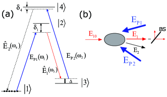
Figure 1: (Color online) (a) Schematic atomic level diagram. $E_{P1}(\omega_{1})$ and $E_{P2}(\omega_{2})$ are the pump fields, and $\hat{E}_{1}(\omega_{3})$ is the probe field. $\hat{E}_{2}(\omega_{4})$ describes the process of another photon $(\omega_{4})$ generated by FWM. (b) Schematic of the experiment for 2+1 photons generation.

Carefully choosing the detuning and intensity of the second pump field, our scheme generates a group of (2+1) photons where two photons are in the same probe frequency mode whereas one photon is in the FWM frequency mode. The schematic of the process is shown in Fig. 1. We consider an ensemble of identical lifetime broadened four-state atoms initially prepared in their ground states $|1\rangle$ by suitable optical pumping method. A cw pump field $(E_{P1})$ couples the ground state $|1\rangle$ to an excited state $|2\rangle$ with a large one-photon detuning $\delta_{1}$. A second strong cw laser field $(E_{P2})$ couples the state $|3\rangle$ to an excited state $|4\rangle$ with the detuning $\Delta+\delta_{4}$. A single-photon probe field $\hat{E}_{1}$ (with central frequency $\omega_{3}$), which couples the state $|2\rangle$ to a lower excited state $|3\rangle$, is then introduced to the medium. Consequently, a two-photon Raman transition can occur, causing an atom to absorb a pump photon and emit a photon into the probe field frequency mode. The presence of the second pump field subsequently pumps the atom to state $|4\rangle$ and a FWM process occurs, leading to the generation of a new photon at the frequency $\omega_{4}=\omega_{1}-\omega_{3}+\omega_{2}$. In such a process two photons at $\omega_{3}$ as well as one photon at $\omega_{4}$ are simultaneously generated, yielding a group of (2+1) correlated photons timing .

The paper is organized as follows. In Sec. II we first derive the equations of motion for atomic dynamics and field propagation equations. With analytical solutions we first examine a limiting case where our scheme reduces to a well-known single $\Lambda$ gain scheme. We then investigate group velocities of various propagation modes and corresponding propagation parameters for the injection-seeded double-$\Lambda$ scheme. In Sec. III, we consider the case where a single-photon quantum probe field is injected into the medium and we investigate the generation of the two probe photons and one FWM photon under the condition of weak gain. We also analyze the two-photon intensity correlation function and coincidence count rate. We also describe the case where the input probe field is a coherent state and obtain the single-photon-added coherent state. In Sec. IV, we show the conversion efficiency of our scheme and compare the efficiencies between our scheme and SPDC case. In Sec. V, we describe how to make our scheme be an alternative approach to generate the photon pair and the possible applications. In Sec. VI, we discuss possible complications due to various ac Stark effects. We also discuss the bandwidth of the Raman gain and the efficiency and bandwidth of single photon source. A summary is given in Sec. VII.

II Model and analysis

II.1 Theoretical model

In the electric-dipole and rotating-wave approximations, the interaction Hamiltonian of $N$ identical four-state atoms interacting with laser fields (see Fig. 1) is given as

$$\hat{H}_{I}^{j}=-\hbar(\Omega_{1}e^{i\vec{k}_{1}\cdot\vec{r}_{j}-i\omega_{1}t}\hat{\sigma}_{21}^{j}+\Omega_{2}e^{i\vec{k}_{2}\cdot\vec{r}_{j}-i\omega_{2}t}\hat{\sigma}_{43}^{j}$$

$$+g_{1}\hat{E}_{1}^{(+)}e^{i\vec{k}_{3}\cdot\vec{r}_{j}-i\omega_{3}t}\hat{\sigma}_{23}^{j}+g_{2}\hat{E}_{2}^{(+)}e^{i\vec{k}_{4}\cdot\vec{r}_{j}-i\omega_{4}t}\hat{\sigma}_{41}^{j}+\mathtt{H.c}),$$

where $\hat{E}_{q}^{(+)}$ is the slowly varying quantum field operator ($q=1,2$ are for probe and FWM field, respectively), $\hat{E}_{q}^{(-)}=(\hat{E}_{q}^{(+)})^{{\dagger}}$, and $\hat{\sigma}_{kl}^{j}=|k\rangle_{jj}\langle l|$ ($k,l=1,2,3,4$). In addition, $2\Omega_{1}=\mu_{21}E_{P1}/\hbar$ and $2\Omega_{2}=\mu_{43}E_{P2}/\hbar$ are Rabi frequencies of pump fields with $\mu_{nn^{\,{}^{\prime}}}$ being the dipole matrix element for the $|n\rangle-|n^{\,{}^{\prime}}\rangle$ transition and $E_{P1,P2}$ being the amplitudes of the two classical pump fields. $g_{1}$ and $g_{2}$ are the atom-photon coupling constants, and $\omega_{m}$ and $\vec{k}_{m}$ $(m=1,2,3,4)$ are the carrier frequency and wave vector of the $m-th$ optical field, respectively.

We define continuum atomic operators $\hat{\sigma}_{\mu\nu}$ by summing over the individual atoms in a small volume $V$, and introduce slowly varying atomic operators $\tilde{\sigma}_{\mu\nu}$: $\sigma_{12}=e^{-i\omega_{1}t}\tilde{\sigma}_{12},\sigma_{13}=e^{i(\omega_{3}-\omega_{1})t}\tilde{\sigma}_{13}=e^{i(\omega_{2}-\omega_{4})t}\tilde{\sigma}_{13},\sigma_{14}=e^{-i\omega_{4}t}\tilde{\sigma}_{14},\sigma_{23}=e^{i\omega_{3}t}\tilde{\sigma}_{23},\sigma_{24}=e^{-i(\omega_{4}-\omega_{1})t}\tilde{\sigma}_{24}=e^{-i(\omega_{2}-\omega_{3})t}\tilde{\sigma}_{24},\sigma_{34}=e^{-i\omega_{2}t}\tilde{\sigma}_{34}$, the equations for the atomic operators in the Heisenberg picture are

$$\dot{\tilde{\sigma}}_{21} = -(\gamma_{21}-i\delta_{1})\tilde{\sigma}_{21}+i\Omega_{1}^{*}e^{-i\vec{k}_{1}\cdot\vec{r}}(\sigma_{22}-\sigma_{11})$$ (2a)

$$+ ig_{2}\hat{E}_{2}^{(-)}e^{-i\vec{k}_{4}\cdot\vec{r}}\tilde{\sigma}_{24}-ig_{1}\hat{E}^{(-)}_{1}e^{-i\vec{k}_{3}\cdot\vec{r}}\tilde{\sigma}_{31},$$

$$\dot{\tilde{\sigma}}_{34} = -(\gamma_{34}+i\delta_{2})\tilde{\sigma}_{34}-i\Omega_{2}e^{i\vec{k}_{2}\cdot\vec{r}}(\sigma_{44}-\sigma_{33})$$ (2b)

$$- ig_{1}\hat{E}_{1}^{(+)}e^{i\vec{k}_{3}\cdot\vec{r}}\tilde{\sigma}_{24}+ig_{2}\hat{E}_{2}^{(+)}e^{i\vec{k}_{4}\cdot\vec{r}}\tilde{\sigma}_{31},$$

$$\dot{\tilde{\sigma}}_{31} = -(\gamma_{31}-i\Delta)\tilde{\sigma}_{31}+i\Omega_{1}^{*}e^{-i\vec{k}_{1}\cdot\vec{r}}\tilde{\sigma}_{32}-i\Omega_{2}e^{i\vec{k}_{2}\cdot\vec{r}}\tilde{\sigma}_{41}$$ (2c)

$$- ig_{1}\hat{E}_{1}^{(+)}\tilde{\sigma}_{21}e^{i\vec{k}_{3}\cdot\vec{r}}+ig_{2}\hat{E}_{2}^{(-)}e^{-i\vec{k}_{4}\cdot\vec{r}}\tilde{\sigma}_{34},$$

$$\dot{\tilde{\sigma}}_{41} = -(\gamma_{41}-i\delta_{4})\tilde{\sigma}_{41}+i\Omega_{1}^{*}e^{-i\vec{k}_{1}\cdot\vec{r}}\tilde{\sigma}_{42}-i\Omega_{2}^{*}e^{-i\vec{k}_{2}\cdot\vec{r}}\tilde{\sigma}_{31}$$ (2d)

$$- ig_{2}\hat{E}_{2}^{(-)}(\sigma_{11}-\sigma_{44})e^{-i\vec{k}_{4}\cdot\vec{r}},$$

$$\dot{\tilde{\sigma}}_{32} = -(\gamma_{32}+i\delta_{3})\tilde{\sigma}_{32}+i\Omega_{1}e^{i\vec{k}_{1}\cdot\vec{r}}\tilde{\sigma}_{31}-i\Omega_{2}e^{i\vec{k}_{2}\cdot\vec{r}}\tilde{\sigma}_{42}$$ (2e)

$$- ig_{1}\hat{E}_{1}^{(+)}(\sigma_{22}-\sigma_{33})e^{i\vec{k}_{3}\cdot\vec{r}},$$

$$\dot{\tilde{\sigma}}_{42} = -[\gamma_{42}-i(\delta_{1}-\delta_{4})]\tilde{\sigma}_{42}+i\Omega_{1}\tilde{\sigma}_{41}e^{i\vec{k}_{1}\cdot\vec{r}}-i\Omega_{2}^{*}\tilde{\sigma}_{32}$$ (2f)

$$\times e^{-i\vec{k}_{2}\cdot\vec{r}}+ig_{1}\hat{E}_{1}^{(+)}\tilde{\sigma}_{43}e^{i\vec{k}_{3}\cdot\vec{r}}$$

$$- ig_{2}\hat{E}_{2}^{(-)}\tilde{\sigma}_{12}e^{-i\vec{k}_{4}\cdot\vec{r}},$$

where $$\delta_{1}=\omega_{21}-\omega_{1},\delta_{2}=\omega_{43}-\omega_{2} \delta_{3}=\omega_{23}-\omega_{3},\delta_{4}=\omega_{41}-\omega_{4} \Delta=\delta_{3}-\delta_{1}=\delta_{2}-\delta_{4} \omega_{kl}=\omega_{k}-\omega_{l} |k\rangle\leftrightarrow|l\rangle \gamma_{kl} \gamma_{kl}=\gamma_{lk} |k\rangle |l\rangle$$, , , and is the frequency of the transition. () is the dephasing rate between state and state .

We consider a pencil-shaped atomic ensemble and assume the atomic sample is optically thin in the transverse direction. Using the slowly varying envelope and unfocused plane-wave approximations, we obtain the following propagation equations for the quantum field operators:

$$\left[\left(c\frac{\partial}{\partial z}+\frac{\partial}{\partial t}\right)\hat{E}_{1}^{(+)}(z,t)\right]e^{i\vec{k}_{3}\cdot\vec{z}}=ig_{1}N\tilde{\sigma}_{32},$$ (3)

$$\left[\left(c\frac{\partial}{\partial z}+\frac{\partial}{\partial t}\right)\hat{E}_{2}^{(-)}(z,t)\right]e^{-i\vec{k}_{4}\cdot\vec{z}}=-ig_{2}N\tilde{\sigma}_{41},$$ (4)

where $N$ is the total number of atoms in the atomic ensemble. Under the condition that the probe field is much weaker than the pump fields, and using the assumption that pump fields propagate without depletion, Eqs. (2a) and (2f) can be evaluated adiabatically,

$$\tilde{\sigma}_{21}^{(0)}\approx\frac{\Omega_{1}^{\ast}e^{-i\vec{k}_{1}\cdot\vec{z}}}{\delta_{1}+i\gamma_{21}},~{}\tilde{\sigma}_{42}^{(0)}\approx\frac{\Omega_{2}^{\ast}\tilde{\sigma}_{32}e^{-i\vec{k}_{2}\cdot\vec{z}}-\Omega_{1}\tilde{\sigma}_{41}e^{i\vec{k}_{1}\cdot\vec{z}}}{\delta_{1}+i\gamma_{42}}.$$ (5)

Considering $\sigma_{22}^{(0)}=\sigma_{33}^{(0)}=\sigma_{44}^{(0)}=\tilde{\sigma}_{34}^{(0)}\approx 0$, and substituting these values of the density matrix elements into Eqs. (2c)-(2e), we obtain the following set of coupled equations:

$$\left\{\begin{aligned} \overset{.}{\tilde{\sigma}}_{31}&=-(\gamma_{31}-i\Delta)\tilde{\sigma}_{31}+i\Omega_{1}^{\ast}e^{-i\vec{k}_{1}\cdot\vec{z}}\tilde{\sigma}_{32}\\ &-i\Omega_{2}e^{i\vec{k}_{2}\cdot\vec{z}}\tilde{\sigma}_{41}-ig_{1}\tilde{\sigma}_{21}\hat{E}_{1}^{(+)}(z,t)e^{i\vec{k}_{3}\cdot\vec{z}},\\ \overset{.}{\tilde{\sigma}}_{41}&=-(\gamma_{41}-i\delta_{4})\tilde{\sigma}_{41}+i\Omega_{1}^{*}e^{-i\vec{k}_{1}\cdot\vec{z}}\tilde{\sigma}_{42}\\ &-i\Omega_{2}^{\ast}e^{-i\vec{k}_{2}\cdot\vec{z}}\tilde{\sigma}_{31}-ig_{2}\hat{E}_{2}^{(-)}(z,t)e^{-i\vec{k}_{4}\cdot\vec{z}},\\ \overset{.}{\tilde{\sigma}}_{32}&=-(\gamma_{32}+i\delta_{3})\tilde{\sigma}_{32}+i\Omega_{1}\tilde{\sigma}_{31}e^{i\vec{k}_{1}\cdot\vec{z}}-i\Omega_{2}e^{i\vec{k}_{2}\cdot\vec{z}}\tilde{\sigma}_{42}.\end{aligned}\right.$$ (6)

Substituting Eq. (5) into Eq. (6), we make the Fourier transform and obtain the solutions for $\tilde{\sigma}_{32}$ and $\tilde{\sigma}_{41}$ in the frequency domain

$$\Sigma_{32} = \frac{g_{1}|\Omega_{1}|^{2}}{d_{1}D(\omega)}[(\omega+d_{4})+\frac{|\Omega_{2}|^{2}-|\Omega_{1}|^{2}}{d_{5}}]\;\hat{\epsilon}_{1}(z,\omega)e^{i\vec{k}_{3}\cdot\vec{z}}$$ (7)

$$+\frac{g_{2}\Omega_{1}\Omega_{2}}{D(\omega)d_{5}}(\omega+d_{5})\;\hat{\epsilon}_{2}^{\dagger}(z,-\omega)e^{i(\vec{k}_{1}+\vec{k}_{2}-\vec{k}_{4})\cdot\vec{z}},$$

$$\Sigma_{41} = -\frac{g_{1}\Omega_{1}^{\ast}\Omega_{2}^{\ast}}{d_{1}D(\omega)}(\omega-d_{3})\;\hat{\epsilon}_{1}(z,\omega)e^{-i(\vec{k}_{1}+\vec{k}_{2}-\vec{k}_{3})\cdot\vec{z}}$$

$$-\frac{g_{2}[(\omega+d_{2})(\omega-d_{3})-|\Omega_{1}|^{2}\ ]}{D(\omega)}\;\hat{\epsilon}_{2}^{\dagger}(z,-\omega)e^{-i\vec{k}_{4}\cdot\vec{z}},$$

where $d_{1}=\delta_{1}+i\gamma_{21}$, $d_{2}=\Delta+i\gamma_{31}$, $d_{3}=\delta_{3}-i\gamma_{32}$, $d_{4}=\delta_{4}+i\gamma_{41}$, $d_{5}=\delta_{1}+i\gamma_{42}$, and $D(\omega)=(\omega+d_{2})(d_{3}-\omega)(\omega+d_{4})+|\Omega_{1}|^{2}(\omega+d_{4})+|\Omega_{2}|^{2}(\omega-d_{3})+|\Omega_{1}\Omega_{2}|^{2}(\omega+2d_{5})/d_{5}^{2}$. Here we ignore some small terms under the condition $\delta_{1}(\delta_{3})\gg\delta_{4},\Delta,\Omega_{1},\Omega_{2}$. In addition, $\hat{\epsilon}_{j}(z,\omega)=\int_{-\infty}^{\infty}\hat{E}_{j}^{(+)}(z,t)e^{i\omega t}dt$, and $\Sigma_{32}(z,\omega)$ and $\Sigma_{41}(z,\omega)$ are Fourier transforms of $\sigma_{32}(z,t)$ and $\sigma_{41}(z,t)$, with $\omega$ being the transform variable, respectively. Making the Fourier transform of Eqs. (3) and (4) and using Eqs. (7) and (II.1) we obtain

$$\frac{\partial}{\partial z}\hat{\epsilon}_{1}(z,\omega) = \frac{i\omega}{c}\hat{\epsilon}_{1}(z,\omega)+iD_{1}(\omega)\hat{\epsilon}_{1}(z,\omega)$$ (9)

$$+iD_{2}(\omega)\hat{\epsilon}_{2}^{\dagger}(z,-\omega)e^{i\Delta\vec{k}\cdot\vec{z}},$$

$$\frac{\partial}{\partial z}\hat{\epsilon}_{2}^{\dagger}(z,-\omega) = \frac{i\omega}{c}\hat{\epsilon}_{2}^{\dagger}(z,-\omega)+iD_{3}(\omega)\hat{\epsilon}_{1}(z,\omega)e^{-i\Delta\vec{k}\cdot\vec{z}}$$ (10)

$$+iD_{4}(\omega)\hat{\epsilon}_{2}^{\dagger}(z,-\omega),$$

where

$$D_{1}(\omega) = \frac{K_{1}|\Omega_{1}|^{2}}{d_{1}d_{5}D(\omega)}[(\omega+d_{4})d_{5}+|\Omega_{2}|^{2}-|\Omega_{1}|^{2}],~{}$$

$$D_{2}(\omega) = \frac{K_{12}\Omega_{1}\Omega_{2}(\omega+d_{5})}{D(\omega)d_{5}},D_{3}(\omega)=\frac{K_{12}\Omega_{1}^{\ast}\Omega_{2}^{\ast}(\omega-d_{3})}{D(\omega)d_{1}},$$

$$D_{4}(\omega) = \frac{K_{2}[(\omega+d_{2})(\omega-d_{3})-|\Omega_{1}|^{2}]}{D(\omega)},$$ (11)

in which $K_{1}=N|g_{1}|^{2}/c,K_{2}=N|g_{2}|^{2}/c,K_{12}=Ng_{1}g_{2}/c,$ and phase mismatch $\Delta\vec{k}=\vec{k}_{4}-\vec{k}_{3}+\vec{k}_{2}-\vec{k}_{1}$. Equations (9) and (10) can be solved analytically for arbitrary initial conditions. For simplicity, we let the phase mismatch $\Delta k=0$. The solutions of Eqs. (9) and (10) are as follows

$$\hat{\epsilon}_{1}(z,\omega) = \frac{1}{U_{+}-U_{-}}[(U_{+}e^{i\lambda_{+}z}-U_{-}e^{i\lambda_{-}z})\hat{\epsilon}_{1}(0,\omega)$$ (12)

$$+ U_{+}U_{-}(e^{i\lambda_{-}z}-e^{i\lambda_{+}z})\hat{\epsilon}_{2}^{\dagger}(0,-\omega)],$$

$$\hat{\epsilon}_{2}^{\dagger}(z,-\omega) = \frac{1}{U_{+}-U_{-}}[(e^{i\lambda_{+}z}-e^{i\lambda_{-}z})\hat{\epsilon}_{1}(0,\omega)$$ (13)

$$+ (U_{+}e^{i\lambda_{-}z}-U_{-}e^{i\lambda_{+}z})\hat{\epsilon}_{2}^{\dagger}(0,-\omega)],$$

where

$$\lambda_{\pm} = \frac{\omega}{c}+\frac{1}{2}[D_{1}(\omega)+D_{4}(\omega)\mp D_{5}(\omega)],$$

$$U_{\pm} = \frac{2D_{2}(\omega)}{D_{4}(\omega)-D_{1}(\omega)\mp D_{5}(\omega)},$$

$$D_{5}(\omega) = \sqrt{(D_{1}(\omega)-D_{4}(\omega))^{2}+4D_{2}(\omega)D_{3}(\omega)}.$$ (14)

We focus our attention on the adiabatic regime Deng1 , where $\lambda_{\pm}$ and $U_{\pm}$ can be expanded into a rapidly converging power series of dimensionless transform variable $\zeta=\omega\tau_{p}$ where $\tau_{p}$ is the pulse duration of the weak probe field. In this regime Deng1 , $U_{\pm}=W_{\pm}+\mathcal{O}(\zeta)$ and $\lambda_{\pm}=(\lambda_{\pm})_{\zeta=0}+\zeta/\tau_{p}V_{g\pm}+\mathcal{O}(\zeta^{2})$ can accurately describe the FWM generation and propagation process. The expansions can be well valid close to the central frequency component of the field. The inverse Fourier transform of Eqs. (12) and (13) is given by

$$\hat{E}_{1}^{(+)}(z,t) = [A_{1}\hat{E}_{1}^{(+)}(\eta_{+})-A_{2}\hat{E}_{2}^{(-)}(\eta_{+})]e^{\beta_{+}z}$$ (15)

$$+[A_{2}\hat{E}_{2}^{(-)}(\eta_{-})-A_{3}\hat{E}_{1}^{(+)}(\eta_{-})]e^{\beta_{-}z},$$

$$\hat{E}_{2}^{(-)}(z,t) = [A\hat{E}_{1}^{(+)}(\eta_{+})-A_{3}\hat{E}_{2}^{(-)}(\eta_{+})]e^{\beta_{+}z}$$ (16)

$$+[A_{1}\hat{E}_{2}^{(-)}(\eta_{-})-A\hat{E}_{1}^{(+)}(\eta_{-})]e^{\beta_{-}z},$$

where$\ A=1/(W_{+}-W_{-})$, $A_{1}=W_{+}A$, $A_{2}=W_{+}W_{-}A$, $A_{3}=W_{-}A$, and $\eta_{\pm}=t-z/V_{g\pm}$, $\beta_{\pm}=i(\lambda_{\pm})_{\omega=0}$ and

$$W_{\pm} = 2D_{2}(0)/(D_{4}(0)-D_{1}(0)\mp D_{5}(0)),$$

$$\beta_{\pm} = i[D_{1}(0)+D_{4}(0)\mp D_{5}(0)]/2,$$

$$\frac{1}{{V_{g}}_{\pm}} = \frac{1}{c}+\frac{D_{1p}(0)+D_{4p}(0)\mp D_{5p}(0)}{2},$$ (17)

in which

$$D_{p}(0) = \left|\Omega_{1}\right|^{2}+\left|\Omega_{2}\right|^{2}+d_{3}d_{4}-d_{2}d_{4}+d_{2}d_{3},$$

$$D_{1p}(0) = \frac{K_{1}|\Omega_{1}|^{2}}{d_{1}d_{5}D(0)}[d_{5}-(d_{4}d_{5}+|\Omega_{2}|^{2}-|\Omega_{1}|^{2})\frac{D_{p}(0)}{D(0)}],$$

$$D_{2p}(0) = -K_{12}\Omega_{1}\Omega_{2}(D(0)+d_{5}D_{p}(0))/d_{5}D^{2}(0),$$

$$D_{3p}(0) = K_{12}\Omega_{1}^{\ast}\Omega_{2}^{\ast}D_{p}(0)(D(0)+d_{3}D_{p}(0))/d_{1}D^{2}(0),$$

$$D_{4p}(0) = \frac{K_{2}}{D^{2}(0)}[(d_{2}-d_{3})D(0)+D_{p}(0)(d_{2}d_{3}+|\Omega_{1}|^{2})],$$

$$D_{5p}(0) = [(D_{1}(0)-D_{4}(0))(D_{1p}(0)-D_{4p}(0))$$

$$+2D_{2p}(0)D_{3}(0)+2D_{2}(0)D_{3p}(0)]/\sqrt{D_{5}(0)}.$$

Here $D_{j}(0)\equiv D_{j}(\omega)|_{\omega=0},(j=1,\cdots,5)$ and $D(0)\equiv D(\omega)|_{\omega=0}$. Equations (15) and (16) indicate that in general each frequency component of the probe and the generated FWM fields contains two propagation modes (wave packets) that travel with different yet individually matched group velocities. In addition, both propagation modes (wave packets) retain a pulse shape identical to that of the input probe field in the adiabatic regime Deng1 .

II.2 Analysis of group velocities and propagation parameters

Figure 2: (Color online) The schematic diagram of fields $\hat{E}_{1}$ and $\hat{E}_{2}$ propagation. Two propagation modes are characterized by the different group velocities ${V_{g}}_{\pm}$ where one mode gains and the other mode attenuates.

Before a detailed analysis we first consider a limiting case where $\Omega_{2}=0$ and $g_{2}=0$. In this limit, our scheme reduces to that of a single $\Lambda$ scheme. Using Eq. (9) we immediately obtain [note that when $g_{2}=0$, $D_{2}(\omega)=0$], thus $\hat{\epsilon}_{1}(z,\omega)=\hat{\epsilon}_{1}(0,\omega)e^{-i\lambda_{0}z}$ where $\lambda_{0}=\omega/c+D_{1}(\omega)$. This leads to a single group velocity

$$V_{g_{0}}=\frac{c}{1-\frac{cK_{1}|\Omega_{1}|^{2}}{d_{1}^{2}d_{2}^{2}}}\approx\frac{-d_{1}^{2}d_{2}^{2}}{K_{1}|\Omega_{1}|^{2}},\left(\left|\frac{cK_{1}|\Omega_{1}|^{2}}{d_{1}^{2}d_{2}^{2}}\right|\gg 1\right).$$ (19)

Alternatively, one can also obtain this result using Eq. (12). Note that with $\Omega_{2}=0$ and $g_{2}=0$, we have $D_{2}(\omega)=D_{3}(\omega)=D_{4}(\omega)=0$, $D_{5}(\omega)=D_{1}(\omega)$, $U_{+}=U_{-}=0$, and $\lambda_{-}=\lambda_{0}=\omega/c+D_{1}(\omega)$ and $\hat{\epsilon}_{1}(z,\omega)=\hat{\epsilon}_{1}(0,\omega)e^{-i\lambda_{0}z}$. Equation (19) is the exact same superluminal group velocity obtained by Payne and Deng Payne in an atomic amplitude treatment of a single $\Lambda$ active-Raman-gain scheme.

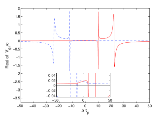
Figure 3: (Color online) Group velocities Re$[V_{g_{+}}/c]$ (solid line) and Re$[V_{g_{-}}/c]$ (dashed line) as function of dimensionless two-photon detuning $\Delta\tau_{p}$ for $K_{1}=K_{2}=K_{12}=1\times 10^{9}$/(m$\cdot$s), $|\Omega_{1}|=\gamma$, $|\Omega_{2}|=5\gamma$, $\tau_{p}=10~{}\mu s$, $\delta_{1}=100\gamma$, $\delta_{4}=0.1\gamma$, $\gamma_{31}=3\times 10^{-5}\gamma$, $\gamma_{21}=\gamma_{23}=\gamma_{41}=\gamma_{43}=\gamma=10$ MHz, and $\gamma_{42}=2\gamma$. The inset shows a magnification of the region for small $V_{g_{+}}$ and $V_{g_{-}}$.

In general, for an injection-seeded double-$\Lambda$ active gain system presented here, each field consists, as indicated in Eqs. (12) and (13), of two propagation modes characterized by the eigenvalues $\lambda_{\pm}$, and therefore different group velocities $V_{g_{\pm}}$ and decay rates. In the adiabatic regime, the propagation of the fields is simply governed by Eqs. (15) and (16). The schematic diagram of fields $\hat{E}_{1}$ and $\hat{E}_{2}$ propagation is showed in Fig. 2. For a short propagation distance where the decay of individual mode is not significant, these modes will overlap each other. Theoretically, for a sufficiently long propagation distance, however, modes with different propagation velocities will separate and the fast decay components decay out completely. Consequently, one obtains a pair of well-matched waves traveling with the identical group velocity and have the identical decay behavior.

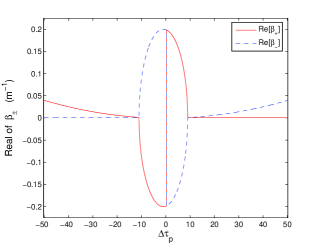
Figure 4: (Color online) The coefficients Re$[\beta_{\pm}]$ versus the dimensionless two-photon detuning $\Delta\tau_{p}$. The parameters are chosen as those using in Fig. 3.

In Fig. 3 we plot group velocities of each propagation mode (wave packet) as a function of dimensionless two-photon detuning $\Delta\tau_{p}$ (i.e., the ratio of two-photon detuning to the bandwidth of the probe field) for a typical cold alkali vapor where states $|2\rangle$ and $|4\rangle$ belong to the same hyperfine manifold. When the two-photon detuning is large, i.e., $\Delta\tau_{p}>22.4$ or $\Delta\tau_{p}<-24.3$ for this specific example, one wave-packet mode travels with a negative (superluminal) group velocity and the other wave-packet mode travels with a positive (subluminal) group velocity that can be substantially smaller than the speed of light in vacuum. In this case, the fast and slow modes separate quickly even before the differential decays become significant. Consequently, one obtains two group velocity-matched probe-FWM field pairs arriving at the detector at a delayed time Deng2 . When the two-photon detuning is small both propagation modes travel with positive group velocities. Under the condition where the two group velocities are equal, one may obtain only one pair of group-velocity matched fields.

To further understand the propagation behavior of probe and generated fields, we examine the propagation parameters $\beta_{\pm}$ in Eqs. (15) and (16). The case of Re[$\beta_{\pm}]>0$ corresponds to gain whereas Re[$\beta_{\pm}]<0$ indicates field attenuation through propagation. In Fig. 4 we show these propagation parameters as functions of the dimensionless two-photon detuning $\Delta\tau_{p}$. In the region ($-10.8<\Delta\tau_{p}<8.8$) where both propagation modes (wave packets) travel with positive group velocities one propagation mode experiences amplification whereas the other propagation mode is attenuated. Note also that near $\Delta\tau_{p}\approx 0.305$ the signs of propagation constant change and the amplified (attenuated) mode becomes attenuated (amplified). These features are very different from the conventional EIT based FWM schemes where probe attenuation and FWM gain always occur. This is precisely due to the fact that EIT process is based on the weak absorption of the probe field and stimulated generation of the FWM field. In the case of active-Raman-gain medium, the probe field serves as an injection seeding source and it works in a stimulated emission mode. Consequently, simultaneous gain to both probe and FWM fields is possible. Indeed, if parameters are chosen such as Re$[\beta_{+}]>0$ and Re$[\beta_{-}]<0$, then after a sufficient propagation distance, both the probe and FWM fields have the same gain feature characterized by Re$[\beta_{+}]>0$. The energy that supports this bi-field increase comes from the two CW classical fields $E_{P1}$ and $E_{P2}$.

III Generation of grouped and paired photons

In this section, we consider the case where the quantum state of the injected probe field corresponds to a single-photon wave-packet state Titulaer ; Raymer :

$$|1\rangle_{\varpi}=\int_{-\infty}^{\infty}d\omega^{{}^{\prime}}P_{p1}(\varpi+\omega^{{}^{\prime}})\hat{a}^{{\dagger}}(\omega^{{}^{\prime}})|0\rangle,$$ (20)

where the amplitudes $P_{p1}(\varpi+\omega^{{}^{\prime}})$ are normalized such that $\int_{-\infty}^{\infty}d\omega^{{}^{\prime}}|P_{p1}(\varpi+\omega^{{}^{\prime}})|^{2}=1$ and the $\varpi$ is central frequency of wave packet. Hence the initial state for the system is

$$|\psi_{in}\rangle=|1\rangle_{3}|0\rangle_{4},$$ (21)

where subscripts $3$ and $4$ denote single photon wave packet of central frequency $\omega_{3}$ and $\omega_{4}$, respectively. In general, the generated quantum state of the system at time $t$ can be expanded in terms of boson Fock space as

$$|\psi_{out}\rangle=\sum_{nm}\alpha_{nm}(t)|n\rangle_{3}|m\rangle_{4},$$ (22)

where $n$ and $m$ denote the photon numbers of the fields with the central frequency $\omega_{3}$ and $\omega_{4}$, respectively and $\sum_{nm}|\alpha_{nm}(t)|^{2}=1$.

When the generated photon numbers $\{n,m\}$ are small enough in the low gain case, we can work out the coefficients $\{\alpha_{nm}\}$ in terms of the moments of the probe and FWM field operators with the forms

$$\langle\psi_{out}|F(\hat{E}_{i}^{(-)}(0),\hat{E}_{i}^{(+)}(0),\hat{E}_{j}^{(-)}(0),$$

$$\hat{E}_{j}^{(+)}(0),\cdots)|\psi_{out}\rangle=\langle\psi_{in}|F(\hat{E}_{i}^{(-)}(L),$$

$$\hat{E}_{i}^{(+)}(L),\hat{E}_{j}^{(-)}(L),\hat{E}_{j}^{(+)}(L),\cdots)|\psi_{in}\rangle,$$ (23)

where $F(\cdots)$ denotes the combinations of products of the field operators required to calculate the coefficients $\{\alpha_{nm}\}$. $\hat{E}_{i}^{(\pm)}(0)$ and $\hat{E}_{i}^{(\pm)}(L)$ are the quantum field operators at the entrance $z=0$ and at the output end $z=L$, respectively.

Figure 5: (Color online) The ratio of ln$|\alpha_{32}|/$ln$|\alpha_{21}|$ versus the $z/z_{m}$ for $\Delta\tau_{p}=-1$ and $z_{m}=1$ cm (solid line). The other parameters are chosen as those using in Fig. 3. The dashed line is for the case the ratio is $2$ (SPDC case).

III.1 Generation and analysis of (2+1) photon group

To generate a (2+1)-group of photons we consider the weak gain limit in which the injected single-probe photon will generate only one photon in the probe frequency mode by stimulated Raman process, accompanied by another photon in the FWM mode. In this case, we only need take account of the low photon numbers: $n,m\in\{0,1,2\}$ in the expansion of Eq. (22). As a result, the final state can be written as

$$|\psi(t)\rangle=\alpha_{10}\left|1\right\rangle_{3}\left|0\right\rangle_{4}+\alpha_{20}\left|2\right\rangle_{3}\left|0\right\rangle_{4}+\alpha_{21}\left|2\right\rangle_{3}\left|1\right\rangle_{4}.$$ (24)

Here, the physical meaning of each term is very clear. $\alpha_{10}$ represents the probability amplitude of the injected single-probe photon not initiating a stimulated emission. $\alpha_{20}$ describes one photon generated through the stimulated emission in the probe mode but without photon generated in the FWM mode. $\alpha_{21}$ is the probability amplitude of one photon generated through the stimulated emission in the probe mode, and simultaneously one photon generated in the FWM mode. The second term in Eq. (24) only exists for a pump field $\Omega_{2}$ which is too weak to excite the FWM process. When the second pump field is strong enough to generate the FWM photon Notation , this amplitude $\alpha_{20}$ tends to zero, and the second term in Eq. (24) vanishes. Further we assume this case to ensure the generation of a (2+1)-group of photons. Then the state vector simply reduces to the form

$$|\psi(t)\rangle=|\alpha_{10}||1\rangle_{3}|0\rangle_{4}+e^{i\phi}|\alpha_{21}||2\rangle_{3}|1\rangle_{4}.$$ (25)

With the help of Eq. (23), one can work out

$$|\alpha_{10}|^{2} = [|A_{1}e^{\beta_{+}L}-A_{3}e^{\beta_{-}L}|^{2}+|A_{2}|^{2}|e^{\beta_{+}L}-e^{\beta_{-}L}|^{2}$$

$$- 4 |A|^{2}|e^{\beta_{+}L}-e^{\beta_{-}L}|^{2}]P_{p1}^{2}(t-L/V_{g}-(z-L)/c),$$

$$|\alpha_{21}|^{2} = 2|A|^{2}|e^{\beta_{+}L}-e^{\beta_{-}L}|^{2}P_{p1}^{2}(t-L/V_{g}-(z-L)/c),$$

$$\phi = \arg[(A_{1}e^{\beta_{+}L}-A_{3}e^{\beta_{-}L})(e^{\beta_{+}L}-e^{\beta_{-}L})^{\ast}A^{\ast}],$$

where we consider the case with the group velocities $V_{g+}=V_{g-}=V_{g}$, and the pulse is assumed to maintain its shape with the profile $P_{p1}(t-L/V_{g}-(z-L)/c)$ during propagation. It is worth of pointing out that for a slightly higher gain, the higher order terms, such as $\alpha_{32}|3\rangle_{3}|2\rangle_{4}$, describing the multiphoton processes will appear in Eq. (25). Similarly, multiphoton processes also exist in the SPDC case in the regime of high gain. For an ideal SPDC case, the quantum state of photons can be expanded in the form $|\psi\rangle=|0\rangle+g|1_{i},1_{s}\rangle+g^{2}|2_{i},2_{s}\rangle+\cdots$, and the probability amplitude of two-photon pairs reduces in the square law for $g<<1$. For comparison, we numerically estimate the corresponding probability amplitude $|\alpha_{32}|$ in our case. The result shown in Fig. 5 indicates that the probability amplitude $|\alpha_{32}|$ has a faster reduction than the square law for a length $z>2.5z_{m}$. This means that our scheme using stimulated Raman process with injection-seeding mechanism is slightly better than the SPDC case for compressing the multiphoton processes, and hence appropriate for generation of single-photon pair.

III.2 Two-photon intensity correlation function and coincidence count rate

To show the time correlation properties of the generated photon pairs, we now work out the Glauber intensity correlation function between the paired photons $(\omega_{3},~{}\omega_{4})$ with a time delay $\tau_{d}$,

$$G_{E_{1}-E_{2}}^{(2)}(\tau_{d})=\langle\hat{E}_{1}^{(-)}(t)\hat{E}_{2}^{(-)}(t+\tau_{d})\hat{E}_{2}^{(+)}(t+\tau_{d})\hat{E}_{1}^{(+)}(t)\rangle.$$ (27)

Note that the correlation function is calculated for the state of two photons (one in probe mode and the other in FWM mode), not the state of three photons. The values $\langle$ $\rangle$ is average of the initial state $|\psi_{in}\rangle=|1\rangle_{3}|0\rangle_{4}=|0\rangle_{4}\int d\omega P_{p1}(-\omega)\epsilon_{1}^{{\dagger}}(0,-\omega)|0\rangle_{3}$ where $P_{p1}(\omega)=1/\sqrt{2\pi}\int_{-\infty}^{\infty}dte^{i\omega t}P_{p1}(t)$ is the pulse shape function of the input photon.

Using the fields operators of Eqs. (12) and (13), one can work out $G_{E_{1}-E_{2}}^{(2)}(\tau_{d})$. In order to denote the result simply, Eqs. (12) and (13) can be written as

$$\hat{\epsilon}_{1}(z,\omega) = R_{1}\hat{\epsilon}_{10}(0,\omega)+S_{1}\hat{\epsilon}_{20}^{\dagger}(0,-\omega),$$ (28)

$$\hat{\epsilon}_{2}^{\dagger}(z,-\omega) = R_{2}\hat{\epsilon}_{10}(0,\omega)+S_{2}\hat{\epsilon}_{20}^{\dagger}(0,-\omega),$$ (29)

and the intensity correlation function $G_{E_{1}-E_{2}}^{(2)}(\tau_{d})$ has been derived as

$$G {}_{E_{1}-E_{2}}^{(2)}(\tau_{d})=\int\int\int\int d\omega_{1}d\omega_{2}d\omega_{3}d\omega_{4}e^{-i\omega_{1}t}$$ (30)

$$\times e^{-i\omega_{2}(t+\tau_{d})}e^{-i\omega_{3}(t+\tau_{d})}e^{-i\omega_{4}t}\langle\hat{\epsilon}_{1}^{\dagger}(z,-\omega_{1})$$

$$\times\hat{\epsilon}_{2}^{\dagger}(z,-\omega_{2})\hat{\epsilon}_{2}(z,\omega_{3})\hat{\epsilon}_{1}(z,\omega_{4})\rangle$$

$$= [\int d\omega P_{p1}^{2}(\omega)|R_{1}|^{2}+\int d\omega|S_{1}|^{2}]\int d\omega|R_{2}|^{2}$$

$$+\int d\omega P_{p1}^{2}|R_{2}|^{2}\int d\omega|S_{1}|^{2}+|\int d\omega e^{i\omega\tau_{d}}S_{1}^{\ast}S_{2}|^{2}$$

$$+\int d\omega e^{-i\omega\tau_{d}}P_{p1}^{2}(\omega)R_{1}^{\ast}R_{2}\times\int d\omega e^{-i\omega\tau_{d}}S_{1}S_{2}^{\ast}$$

$$+\int d\omega e^{i\omega\tau_{d}}P_{p1}^{2}(\omega)R_{1}R_{2}^{\ast}\times\int d\omega e^{i\omega\tau_{d}}S_{1}^{\ast}S_{2}$$

$$\approx G_{E_{1}}^{(1)}(0)G_{E_{2}}^{(1)}(0)+|\int d\omega e^{i\omega\tau_{d}}S_{1}^{\ast}S_{2}|^{2}$$

$$+\int d\omega e^{-i\omega\tau_{d}}P_{p1}^{2}(\omega)R_{1}^{\ast}R_{2}\times\int d\omega e^{-i\omega\tau_{d}}S_{1}S_{2}^{\ast}$$

$$+\int d\omega e^{i\omega\tau_{d}}P_{p1}^{2}(\omega)R_{1}R_{2}^{\ast}\times\int d\omega e^{i\omega\tau_{d}}S_{1}^{\ast}S_{2}.$$

The second-order normalized intensity correlation function is $g_{E_{1}-E_{2}}^{(2)}(\tau_{d})=G_{E_{1}-E_{2}}^{(2)}(\tau_{d})/G_{E_{1}}^{(1)}(0)G_{E_{2}}^{(1)}(0)$ where the peak value of normalized $g_{E_{1}-E_{2}}^{(2)}\gg 1$, the antibunching nature, which implies a finite time delay for the emission of the second quantum field photon $(\omega_{4})$. In other words, a nonclassical photon pair composed of frequencies $\omega_{3}$ and $\omega_{4}$ is generated in atomic vapors.

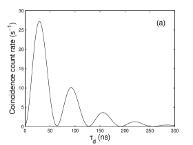
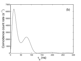
Figure 6: Coincidence count rate in a $1$ ns bin versus the delay time $\tau_{d}$ for $\Delta\tau_{p}=-1$ and $z/z_{m}=5$ at (a) $K=2\times 10^{8}$/(m$\cdot$s) and (b) $K=3\times 10^{9}$/(m$\cdot$s). The other parameters are chosen as those using in Fig. 3.

The coincidence count rate $R_{c}(\tau_{d})$ is obtained from the intensity correlation function as $R_{c}(\tau_{d})=\epsilon^{2}\Delta TG_{E_{1}-E_{2}}^{(2)}(\tau_{d})$ with a bin size $\Delta T=1$ ns much smaller than the correlation time. The factor $\epsilon$ accounts for the photon counter efficiency, the filter transmission, and fiber coupling. In Fig. 6, we show the coincidence count rate $R_{c}(\tau_{d})$ in a $1$ ns bin depending on the $K$. When $K$ is small, which occurs, for example, at low optical depth, the atomic system behaves like a single atom. In such a regime the intensity correlation function reveals the damped Rabi oscillations. By increasing the optical depth of the atomic sample, it becomes possible to achieve the $E_{1}$-$E_{2}$ correlation function with shorter time.

III.3 Single-photon added coherent state

Another possible extension of the stimulated Raman process with injected seed is to generate a single-photon added coherent state (SPACS) Agarwal . For this purpose, we consider injection of a weak coherent state $|\alpha\rangle_{3}$ into the medium instead of a probe single photon $|1\rangle_{3}$. Here, we also consider the weak gain limit where only one photon will be generated into the probe field by stimulated Raman process, accompanied by another photon in the FWM mode. With such an arrangement, we have the output state

$$\ |\psi\rangle=\beta_{1}|\alpha\rangle_{3}|0\rangle_{4}+\beta_{2}|\alpha,1\rangle_{3}|1\rangle_{4}.$$ (31)

When only a single photon in the frequency $\omega_{4}$ is detected, the state $|\psi\rangle$ will collapse to the SPACS $|\alpha,1\rangle$. The schematic is shown in Fig. 7. Again, our scheme using stimulated Raman process in atomic ensemble offers a direction-controllable way to generate a SPACS, compared to the present method demonstrated in the nonlinear crystal Zavatta .

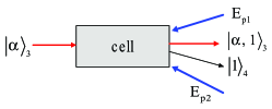
Figure 7: (Color online) The schematic of generating single-photon added coherent state (SPACS).

IV Conversion efficiency

In this section, we come to evaluate the output conversion efficiency of our photon pair. The intensity of the fields is given by Boyd

$$I=2n(\varepsilon_{0}/\mu_{0})^{1/2}|E|^{2}.$$ (32)

where $\varepsilon_{0}=8.85\times 10^{-12}$ F/m, $\mu_{0}=4\pi\times 10^{-7}$ H/m, and $n$ is the refractive index, and $E$ is measured in V/m. First, we calculate the intensities of pump fields $E_{P1}$ and $E_{P2}$. The relations of Rabi frequencies of pump fields with the transition matrix element are $2\Omega_{1}=\mu_{21}E_{P1}/\hbar$ and $2\Omega_{2}=\mu_{43}E_{P2}/\hbar$, so the intensity of $I_{Pj}$ in the undepleted pump approximation ($I_{Pj}(z)=I_{Pj}(0)$) is

$$I_{Pj}(0)=8n_{j}(\varepsilon_{0}/\mu_{0})^{1/2}|\hbar\Omega_{j}/\mu_{j}|^{2},\text{ \ }j=\{1,2\},$$ (33)

where $\mu_{1}$ and $\mu_{2}$ denote $\mu_{21}$ and $\mu_{43}$, respectively.

Next, the intensities of generation fields $E_{1}$ and $E_{2}$ at the boundary $L$ are

$$I_{E_{j}}=I_{0_{j}}\langle\hat{E}_{j}^{(-)}\hat{E}_{j}^{(+)}\rangle,\text{ \ \ \ }j=\{1,2\},$$ (34)

where $I_{0_{j}}=(\sqrt{\hbar\omega_{2+j}/2\varepsilon_{0}A_{\text{eff}}c\tau_{p}})^{2}$ ($j=1,2)$ Payne03 and $A_{\text{eff}}$ is the effective beam cross section, and the fields $\hat{E}_{1}$ and $\hat{E}_{2}$ are described by Eqs. (15) and (16) and average over initial the state $|1\rangle_{3}|0\rangle_{4}$. We consider the general case: only one of two modes $\beta_{+}$ and $\beta_{-}$ is obtained, such as $\beta_{+}$, then the peak intensity of the field $I_{E_{1}}$ is

$$I_{E_{1}}(L)=\frac{\hbar\omega_{3}}{2\varepsilon_{0}A_{\text{eff}}c\tau_{p}}[|A_{1}|^{2}+|A_{2}|^{2}]|e^{\beta_{+}L}|^{2},$$ (35)

and the peak intensity of the field $I_{E_{2}}$ under the same condition is

$$I_{E_{2}}(L)\simeq\frac{\hbar\omega_{4}}{\varepsilon_{0}A_{\text{eff}}c\tau_{p}}|A|^{2}|e^{\beta_{+}L}|^{2}.$$ (36)

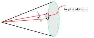
Figure 8: (Color online) The light emitted by SPDC experiment is collected from a small portion of solid angle.

The ideal efficiency $\eta_{j}$ ($j=1,2$) for conversion of power from the pump photons $\omega_{j}$ ($j=1,2$) to the photons $\omega_{2+j}$ ($j=1,2$) is

$$\eta_{1}=\frac{P_{3}(L)}{P_{1}(0)}=\frac{I_{E_{1}}(L)}{I_{P1}(0)},\text{ \ }\eta_{2}=\frac{P_{4}(L)}{P_{2}(0)}.$$ (37)

Considering the efficiency of the present available single-photon source $\eta_{s}\approx 9\%$ Hijlkema , we can have the total conversion efficiencies in our scheme $\eta_{\text{tot}_{j}}$ ($j=1,2$) is

$$\eta_{\text{tot}_{j}}=\eta_{j}\eta_{s},\text{ \ }j=\{1,2\}.$$ (38)

Now, we numerically evaluate the total conversion efficiency $\eta_{\text{tot}_{j}}$. As a numeric example with a particular ⁸⁷Rb atomic ensemble using, we assume the hyperfine levels involved: $\{|5^{2}S_{1/2},F=1,m_{F}=1\rangle,~{}|5^{2}S_{1/2},F=2,m_{F}=1\rangle,~{}|5^{2}P_{1/2},F^{\prime}=2,m_{F^{\prime}}=0\rangle$,  $|5^{2}P_{3/2},F^{\prime}=2,m_{F^{\prime}}=2\rangle\}$, which correspond to the levels $\{|1\rangle,~{}|3\rangle,~{}|2\rangle,~{}|4\rangle\}$ in our scheme. As a result, the transition dipole matrix elements $|\mu_{21}|=2.992$ $ea_{0}/\sqrt{12}$ and $|\mu_{43}|=4.227$ $ea_{0}/\sqrt{12}$, and the excited transitions $|2\rangle\rightarrow|3\rangle$ and $|4\rangle\rightarrow|1\rangle$ have the same Clebsch-Gordon coefficient $1/2$ Steck . The spot sizes of the probe and FWM laser beams $w_{0}$ are assumed to the same with $w_{0}\simeq 10$ $\mu$m in our calculation. The dimensionless two-photon detuning is chosen as $z=5z_{m}$ and $\Delta\tau_{p}=3$ corresponding to $\beta_{+}$ mode and the other parameters are chosen as the same as those using in the Fig. 3. Finally, we have the total conversion efficiencies for the atomic ensemble,

$$\eta_{\text{tot}_{1}}\approx 5.919\times 10^{-8}/\text{cm},$$ (39)

and

$$\eta_{\text{tot}_{2}}\approx 4.819\times 10^{-9}/\text{cm}.$$ (40)

For comparison, we also examine the conversion efficiency for the generation of photon pairs in SPDC case. A SPDC process is described by the Hamiltonian, $\hat{H}=i\hbar\eta A_{p}\hat{a}_{s}^{{\dagger}}\hat{a}_{i}^{{\dagger}}+$H.c.,with a strong classical field $A_{p}$ and the weak signal (idler) field $\hat{a}_{s}^{{\dagger}}$ ($\hat{a}_{i}^{{\dagger}}$). The output state in SPDC case can be approximated as $|\psi(t)\rangle=|0\rangle+g|1_{s},1_{i}\rangle$ for $g=\eta A_{p}t<<1$. The conversion efficiency of pump photons into correlated photon pairs integrated over all emission directions is on the order of $3\times 10^{-8}$ mm^-1sr^-1 for a typical nonlinear material Klyshko ; Ling08 . However, in practical operation, one photodetector can only collect photons from a small portion of solid angle as shown in Fig. 8. For example, in the experimentLing08 , the collection angle is $3.3\times 10^{-5}$ sr. This leads to a realistic conversion efficiency is about $1\times 10^{-12}$ mm^-1 of crystal length. Taking account of the reduction of efficiency due to collection angle in real detection for SPDC case, it is evident that the overall conversion efficiency in our case will be higher due to the determined direction of emitted photons by stimulated process. In this sense, our scheme can have some merits over SPDC case and provide a different method to generate photon pairs using atomic system.

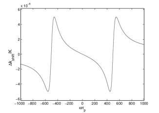
Figure 9: Phase mismatching induced by Stark shift $\Delta k_{\mathtt{shift}}$ as function of detuning $\omega\tau_{p}$ for $\Delta\tau_{p}=-1$. The other parameters are chosen as those using in Fig. 3.

V Applications of (2+1) photon source

In the section, we explore the possibilities for applications of our scheme. Firstly, the scheme can be used to generate photon pair due to the existence of the second term on the right side in Eq. (25). This term represents the situation of simultaneous existence of two photons in the probe frequency mode ($\omega_{3}$) and one photon in the FWM frequency mode ($\omega_{4}$). Detection of a trigger photon ($\omega_{3}$) will project this state into $|\phi\rangle=\alpha_{10}|0\rangle_{3}|0\rangle_{4}+e^{-i\phi}\alpha_{21}|1\rangle_{3}|1\rangle_{4}$. In the weak gain limit considered in the paper this state $|\phi\rangle$ has a large vacuum component $\alpha_{10}$ and a small admixture of the two photon state $\alpha_{21}$. Such a state shares a great similarity to that generated in SPDC experiments. Despite such a similarity between our scheme and the SPDC case, our scheme in generating photon pairs has its own reason for specialty. For example, the frequency of generated photon pairs can be widely tuned. The conversion efficiency can be achieved effectively higher than SPDC case due to the injection-seed mechanism and stimulated Raman process. The injection-seed mechanism ensures a highly directional photon emission which can increase the collecting efficiency of photons in the detection, compared to SPDC case. Stimulated Raman process somehow increases the emission probability. This is because, for an $N$-photon state input, we have the term $\hat{a}_{k}^{{\dagger}}\hat{a}_{l}^{{\dagger}}|N\rangle_{k}|0\rangle_{l}=\sqrt{N+1}|N+1\rangle_{k}|1\rangle_{l}$. As a result, the photon emission probability is $N+1$ times that of the spontaneous emission described by ($\hat{a}_{k}^{{\dagger}}\hat{a}_{l}^{{\dagger}}|0\rangle_{k}|0\rangle_{l}=|1\rangle_{k}|1\rangle_{l}$) Ou08 . Though the enhancement is low for our case limited by $N=1$, the generation probability is $2$ times of that from spontaneous emission. Furthermore, the one-photon emission enhancement due to stimulated emission was observed by Lamas-Linares et al. Lamas-Linares . On the other hand, what is more important is that if a perfect single photon is on demand, the conversion efficiency from pump photons into photon pairs will be significantly improved in our scheme. Hence our scheme can have the potential to take over the SPDC case if the single-photon-on-demand source is available in the future.

In additional to the generation of photon pairs, our (2+1) photon source can also be used to generate photon-number Fock state for quantum communication and other applications. Recently, Ou Ou08 presented a scheme with a number of ideas for efficient conversion between photons. In the scheme, one of the ideas is to use the four-wave mixing as a two-photon annihilator, the input of which requires a two-photon Fock state. Our (2+1) photon source can be a candidate for providing such a two-photon Fock state by projecting the state $|\psi(t)\rangle$ described in Eq. (25) into the state $|2\rangle_{3}$ with the detection of the trigger photon $|1\rangle_{4}$.

Figure 10: Frequency-dependent gain coefficient for the probe field as function of detuning $\omega\tau_{p}$ for $\Delta\tau_{p}=-1$. The other parameters are chosen as those using in Fig. 3.

VI Discussion

In this section we first discuss these ac Stark-type frequency shifts. From Eqs. (9) and (10), we obtain the phase mismatching induced by Stark shift

$$\Delta k_{\mathtt{shift}}=\mathtt{Re}[D_{1}(\omega)-D_{4}(\omega)].$$ (41)

Figure 9 shows phase mismatching induced by the Stark shift versus $\omega\tau_{p}$ by numerical calculations. It is clear from a comparison between Figs. 9 and 10 that the mismatching $\Delta k_{\mathtt{shift}}$ induced by Stark shift is very small with the exclusion of two maximal phase mismatches that occur in the regions where the gain coefficients are maximized. From Fig. 9 we also obtain that the magnitude of two maximal phase mismatches are small compared with that of the wave vector of light field, so the angle of departure of field $\hat{E}_{2}$ from the direction determine by $\Delta\vec{k}\cdot\vec{z}\approx 0$ is small.

Once the single-photon probe field is introduced, we can generate a correlated photon pair with probability $|\alpha_{21}|^{2}/2$ when only one photon $|1\rangle_{3}$ is detected. In order to obtain the desired result, the Raman gain (by the pump field Rabi frequency $\Omega_{1}$) should be kept very low to ensure the stimulated generation of one probe photon. Of course, the pump field Rabi frequency $\Omega_{2}$ should be kept appropriately to ensure the unit conversion from state $|3\rangle$ to state $|4\rangle$ which leads to the simultaneous generation of one FWM photon. Figure 9 depicted the Raman gain in the Fourier transform space for the parameters used. As expected, the gain is small and rather flat as required under the condition that the $\omega\tau_{p}$ is small.

We further note that with sufficient $\Omega_{2}$ our scheme has approximately a EIT-like behavior, as can be seen from Hamiltonian (II.1). In this case, our four-level system is a hybrid system which is composed of an effective EIT (for the FWM photon generation) and Raman gain (for the probe photon generation). Specifically, consider the limiting case where $\delta_{4}=0$, $\Delta=0$, $|\Omega|=|\Omega_{1}|=|\Omega_{2}|$, and very large one-photon detuning $\delta_{1}$, we find that the group velocity $1/{V_{g}}=1/{V_{g}}_{+}=1/{V_{g}}_{-}\approx 1/c+K/(2|\Omega|^{2})$ which is EIT-like.

Next, we discuss the bandwidth of the Raman gain and the spatial width of single photons wave packet. From Fig. 10 we know the magnitude of Raman gain bandwidth is 10 MHz. The injecting seed single-photon wave-packet should be microsecond or sub-microsecond pulse. Such single photon source has so far only been achieved with radiating object (atoms, quantum dots) in high-finesse microcavities because the efficiency of single photon source is hard to obtain high in free space due to the light-collecting lens covers only a fraction of the full 4$\pi$ solid angle. Using a single atom makes it possible to produce single photons with controlled waveform Kuhn ; McKeever ; Keller ; Hijlkema and polarization Wilk , which allows realizing deterministic protocols in quantum information science Wilk2 . The deterministic and high efficient single-photon source Hijlkema ; Wilk ; Matsukevich06 ; Chen06 can support the present scheme. The single-photon-generation probability is about $9\%$ by Rempe group Hijlkema . The low efficiency of single photon sources degrades our scheme. When a perfect single source is on demand our scheme will have potential applications.

Finally, we point out that the effect of quantum noises from the atomic system is ignored since the terms of Langevin-noise operators are excluded in Eq. (2). The ignorance of quantum noises is valid here as we exploit only the low-gain regime of the active-Raman-gain medium for the purpose of generation of correlated photons.

VII Conclusion

In conclusion, we have studied a (2+1)-photon generation scheme using a life-time broadened four-state atomic system. This scheme is based on a double-$\Lambda$ excitation configuration with the first $\Lambda$ branch forming an active-Raman-gain medium. This is very different from the conventional SPDC scheme. Furthermore, it is different from the spontaneous emission based biphoton generation scheme because of the injection-seeding mechanism. This injection-seeding technique leads to the highly directional generation of desired photons, resulting in high detection efficiency. An important feature of the present scheme is that two identical probe photons, because of the stimulated Raman emission process due to injection-seeding, and a FWM photon are generated simultaneously, yielding correlated and entangled (2+1) photons. Consequently, one of the probe photons can be used as a coincidence trigger whereas the remaining probe and FWM photons form a correlated or entangled pair that allows further experimental studies of paired propagation. In addition, (2+1)-photon source can also be used to generate photon-number Fock state. Hence if the single-photon-on-demand source is available in the future, our scheme can have the potential to take over the SPDC case and have potential applications.

References

- (1) A. Kuzmich, W. P. Bowen, A. D. Boozer, A. Boca, C. W. Chou, L.-M. Duan, and H. J. Kimble, Nature 423, 731 (2003); S. V. Polyakov, C. W. Chou, D. Felinto, and H. J. Kimble, Phys. Rev. Lett. 93, 263601 (2004).
- (2) C. H. van der Wal, M. D. Eisaman, A. André, R. L. Walsworth, D. F. Phillips, A. S. Zibrov, and M. D. Lukin, Science 301, 196 (2003).
- (3) D. N. Matsukevich and A. Kuzmich, Science 306, 663 (2004).
- (4) V. Balić, D. A. Braje, P. Kolchin, G.Y. Yin, and S. E. Harris, Phys. Rev. Lett. 94, 183601 (2005).
- (5) P. Kolchin, S. Du, C. Belthangady, G. Y. Yin, and S. E. Harris, Phys. Rev. Lett. 97, 113602 (2006).
- (6) J. K. Thompson, J. Simon, Huanqian Loh, V. Vuletić, Science 313, 74 (2006).
- (7) Shengwang Du, Jianming Wen, Morton H. Rubin, and G.Y. Yin, Phys. Rev. Lett. 98, 053601 (2007).
- (8) Qiang Zhang, Xiao-Hui Bao, Chao-Yang Lu, Xiao-Qi Zhou, Tao Yang, Terry Rudolph, and Jian-Wei Pan, Phys. Rev. A 77, 062316 (2008).
- (9) M. G. Payne and L. Deng, Phys. Rev. A 64, 031802(R) (2001). Note for we have .
- (10) K. J. Jiang, L. Deng, and M. G. Payne, Phys. Rev. A 74, 041803(R) (2006).
- (11) L. Deng and M. G. Payne, Phys. Rev. Lett. 98, 253902 (2007).
- (12) L. J. Wang, A. Kuzmich, and A. Dogariu, Nature (London) 406, 277 (2000).
- (13) It should be noted that the strong and far-detuned pump field can still generate a very weak spontaneous Raman emission at the frequency near the frequency of when the probe field is absent (in the vacuum state) in the atomic medium. This process, however, can be distinguished and discriminated by the usual time-gating techniques. The Raman gain due to the first pump field should be small in order to generate only one photon in stimulated process.
- (14) L. Deng, M. G. Payne, G.X. Huang, and E.W. Hagley, Phys. Rev. E 72, 055601(R) (2005); Y. Wu, M.G. Payne, E.W. Hagley, and L. Deng, Phys. Rev. A70, 063812 (2004).
- (15) L. Deng, M.G. Payne, and E.W. Hagley, Phys. Rev. A70, 063813 (2004).
- (16) U. M. Titulaer and R. J. Glauber, Phys. Rev. 145, 1041 (1966).
- (17) M. G. Raymer, Jaewoo Noh, K.Banaszek, and I.A.Walmsley, Phys. Rev. A 72, 023825 (2005).
- (18) This requires a to be on the order of and larger than .
- (19) G. S. Agarwal, and K. Tara, Phys. Rev. A 43, 492 (1991).
- (20) A. Zavatta, S. Viciani, and M. Bellini, Science 306, 660 (2004).
- (21) R.W. Boyd, Nonlinear Optics (Academic Press, San Diego, 2003), pp. 565-568.
- (22) M. G. Payne and L. Deng, Phys. Rev. Lett. 91, 123602 (2003).
- (23) M. Hijlkema, B. Weber, H. P. Specht, S. C. Webstern, A. Kuhn, and G. Rempe, Nature Phys. 3, 253 (2007).
- (24) For details of the transition probabilities of D line in Rb87, see http://steck.us/alkalidata.
- (25) D. N. Klyshko, Photons and Nonlinear Optics (Gordon and Breach Science Publishers, New York, 1988).
- (26) A. Ling, A. Lamas-Linares, and C. Kurtsiefer, Phys. Rev. A 77, 043834 (2008).
- (27) F. W. Sun, B. H. Liu, Y. X. Gong, Y. F. Huang, Z. Y. Ou, and G. C. Guo, Phys. Rev. Lett. 99, 043601 (2007); Z. Y. Ou, Phys. Rev. A 78, 023819 (2008).
- (28) A. Lamas-Linares, C. Simon, J.C. Howell, and D. Bouwmeester, Science 296, 712 (2002).
- (29) A. Kuhn, M. Hennrich, G. Rempe, Phys. Rev. Lett. 89, 067901 (2002).
- (30) J. McKeever, A. Boca, A. D. Boozer, R. Miller, J. R. Buck, A. Kuzmich, H. J. Kimble, Science 303, 1992 (2004).
- (31) M. Keller, B. Lange, K. Hayasaka, W. Lange, H. Walther, Nature 431, 1075 (2004).
- (32) T. Wilk, S. C. Webster, H. P. Specht, G. Rempe, A. Kuhn, Phys. Rev. Lett. 98, 063601 (2007).
- (33) T. Wilk, S. C. Webster, A. Kuhn, G. Rempe, Science 317, 488 (2007).
- (34) D. N. Matsukevich, T. Chanelière, S. D. Jenkins, S.-Y. Lan, T. A. B. Kennedy, and A. Kuzmich, Phys. Rev. Lett. 97, 013601 (2006).
- (35) S. Chen, Y. A. Chen, T. Strassel, Z. S. Yuan, B. Zhao, J. Schmiedmayer, and J. W. Pan, Phys. Rev. Lett. 97, 173004 (2006).