Topological properties of Abelian and non-Abelian quantum Hall states
from the pattern of zeros

Abstract

It has been shown that different Abelian and non-Abelian fraction quantum Hall states can be characterized by patterns of zeros described by sequences of integers $\{S_{a}\}$. In this paper, we will show how to use the data $\{S_{a}\}$ to calculate various topological properties of the corresponding fraction quantum Hall state, such as the number of possible quasiparticle types and their quantum numbers, as well as the actions of the quasiparticle tunneling and modular transformations on the degenerate ground states on torus.

I Introduction

Characterization and classification of wave functions with infinite variables are the key to gain a deeper understanding of quantum phases and quantum phase transitions. For a long time, people have used symmetry properties of the wave functions and the change of those symmetries to understand quantum phases and quantum phase transitions. However, the discovery of fractional quantum Hall (FQH) states Tsui et al. (1982); Laughlin (1983) suggests that the symmetry characterization is not enough to describe different FQH states. Thus FQH states contain a new kind of order – topological order.Wen and Niu (1990); Wen (1995) Topological order is so new that the conventional mathematical tools and the language developed for symmetry breaking orders are not adequate to describe it. Thus, looking for new mathematical framework to describe the topological order becomes an important task in advancing the theory of topological order.Freedman et al. (2004); Levin and Wen (2005); Kitaev (2006); BK Intuitively, topological order correspond to pattern of long-range quantum entanglement in the ground state, as revealed by the topological entanglement entropy.Kitaev and Preskill (2006); Levin and Wen (2006) Characterizing topological order is characterizing patterns of long-range entanglement.

In a recent paper,WWsymm the pattern of zeros is introduced to characterize and classify symmetric polynomials of infinite variables. Applying this result to FQH states, we find that the pattern of zeros characterizes and classifies many Abelian and non-Abelian FQH states. In other words, the pattern of zeros characterizes the topological order in FQH states.Wen (1995) This may lead to a deeper understanding of topological order in FQH states.

More concretely, a pattern of zeros that characterizes FQH ground state wave functions is described a sequence of integers $\{S_{a}\}$. Describing pattern of zeros through a sequence of integers $\{S_{a}\}$ generalizes the pseudo potential construction of ideal Hamiltonian and the associated zero-energy ground state.Haldane (1983); Greiter et al. (1992); Wen (1993); Read and Rezayi (1999); Read (2006); Simon et al. (2007) All the topological properties of FQH states should be determined by the data $\{S_{a}\}$. In this paper, we will show how to use the data $\{S_{a}\}$ to calculate those topological properties. They include the quantum number of possible quasiparticles and the ground state degeneracy on torus.Haldane (1985); Wen (1989) We also study the actions of quasiparticle tunneling and the modular transformation on the degenerate ground states.Wen (1990) The main results of the paper are summarized in Section V.

II Fusion and pattern of zeros

In LABEL:WWsymm, we have introduced the pattern of zeros of a wave function by bringing $a$ variables together. In this section, we will review the pattern of zeros within such an approach, but from a slightly different angle. For readers who are interested in the new results can go directly to section III.

II.1 Fusion of $a$ variables

To bring $a$ variables in a symmetric polynomial $\Phi(\{z_{i}\})$ together, let us view $z_{1},\cdots,z_{a}$ as variables and $z_{a+1},z_{a+2},\cdots$ as fixed parameters. We write $\Phi(z_{1},z_{2},\cdots)$ as

$$\Phi(\{z_{i}\})=\Phi(z_{1},\cdots,z_{a};z_{a+1},z_{a+2},\cdots)$$

where $\Phi(z_{1},\cdots,z_{a};z_{a+1},z_{a+2},\cdots)$ is a symmetric polynomial of $z_{1},\cdots,z_{a}$ parameterized by $(z_{a+1},z_{a+2},\cdots)$. Now let us rewrite

$$z_{i} =\lambda\xi_{i}+z^{(a)},\ \ \ z^{(a)}=\frac{z_{1}+\cdots+z_{a}}{a},$$

$$\sum_{i=1}^{a}\xi_{i}=0,\ \ \ i=1,\cdots,a,$$

and expand $\Phi(\lambda\xi_{1}+z^{(a)},\cdots,\lambda\xi_{a}+z^{(a)};z_{a+1},z_{a+2},\cdots)$ in powers of $\lambda$:

$$\ \ \ \Phi(\lambda\xi_{1}+z^{(a)},\cdots,\lambda\xi_{a}+z^{(a)};z_{a+1},z_{a+2},\cdots)$$

$$=\sum_{m=0}^{\infty}\lambda^{m}P_{m}[z^{(a)},(\xi_{1},\cdots,\xi_{a});z_{a+1},z_{a+2},\cdots]$$

where $P_{m}[z^{(a)},(\xi_{1},\cdots,\xi_{a});z_{a+1},z_{a+2},\cdots]$ is a homogenous symmetric polynomial of $\xi_{1},\cdots,\xi_{a}$ of degree $m$. $P_{m}[z^{(a)},(\xi_{1},\cdots,\xi_{a});z_{a+1},z_{a+2},\cdots]$ is also a polynomial of $z^{(a)}$ and $z_{a+1},z_{a+2},\cdots$. The minimal power of $z^{(a)}$ is zero.

The polynomial $P_{m}[z^{(a)},(\xi_{1},\cdots,\xi_{a});z_{a+1},z_{a+2},\cdots]$ is derived from $\Phi(\{z_{i}\})$ after fusing $a$ $z_{i}$-variables into a single $z^{(a)}$ variable. Different choices of $\xi_{1},\cdots,\xi_{a}$ represent different ways to fuse $z_{1},\cdots,z_{a}$ into $z^{(a)}$. As a polynomial of $z^{(a)},z_{a+1},z_{a+2},\cdots$, different ways of fusion can produce linearly independent $P_{m}[z^{(a)},(\xi_{1},\cdots,\xi_{a});z_{a+1},z_{a+2},\cdots]$. Thus $(\xi_{1},\cdots,\xi_{a})$ can be viewed as a label for those linearly independent polynomials of $z^{(a)},z_{a+1},z_{a+2},\cdots$.

$P_{m}[z^{(a)},(\xi_{1},\cdots,\xi_{a});z_{a+1},z_{a+2},\cdots]$ is also a symmetric polynomial of $\xi_{1},\cdots,\xi_{a}$. Different $z^{(a)},z_{a+1},z_{a+2},\cdots$ also lead to different symmetric polynomials of $\xi_{1},\cdots,\xi_{a}$. Let $K_{a,m}$ be the number of linearly independent symmetric polynomials of $\xi_{1},\cdots,\xi_{a}$, $P_{m}[z^{(a)},(\xi_{1},\cdots,\xi_{a});z_{a+1},z_{a+2},\cdots]$, produced by all the choices of $z^{(a)},z_{a+1},z_{a+2},\cdots$. Let $F^{(m)}_{\alpha^{(a)}}(\xi_{1},\cdots,\xi_{a})$ be a basis of those symmetric polynomials of $\xi_{1},\cdots,\xi_{a}$, where $\alpha^{(a)}=1,2,\cdots,K_{a,m}$ label those linearly independent symmetric polynomials of $\xi_{1},\cdots,\xi_{a}$. Thus the different polynomials of $z^{(a)},z_{a+1},z_{a+2},\cdots$ labeled by $(\xi_{1},\cdots,\xi_{a})$ can be written as

$$\ \ \ P_{m}[z^{(a)},(\xi_{1},\cdots,\xi_{a});z_{a+1},z_{a+2},\cdots]$$

$$=\sum_{\alpha^{(a,m)}=1}^{K_{a,m}}F^{(m)}_{\alpha^{(a,m)}}(\xi_{1},\cdots,\xi_{a})P_{m}[z^{(a)},\alpha^{(a)};z_{a+1},z_{a+2},\cdots]$$

We see that as different polynomials of $z^{(a)},z_{a+1},z_{a+2},\cdots$ labeled by $\xi_{1},\cdots,\xi_{a}$, $P_{m}[z^{(a)},(\xi_{1},\cdots,\xi_{a});z_{a+1},z_{a+2},\cdots]$ can also be labeled by $\alpha^{(a,m)}$. $F^{(m)}_{\alpha^{(a,m)}}(\xi_{1},\cdots,\xi_{a})$ can be viewed as a conversion factor between the two different labels, $\alpha^{(a,m)}$ and $\xi_{1},\cdots,\xi_{a}$.

Let $S_{a}$ be the minimal total power of $z_{1},\cdots,z_{a}$ in $\Phi(\{z_{i}\})$. We see that $K_{a,m}=0$ if $m<S_{a}$, and

$$K_{a}\equiv K_{a,S_{a}}\neq 0.$$

Since the symmetric polynomial $F^{(m)}_{\alpha^{(a,m)}}(\xi_{1},\cdots,\xi_{a})$ of order $m=1$ must have a form

$$F^{(m=1)}_{\alpha^{(a,m)}}(\xi_{1},\cdots,\xi_{a})\propto\sum\xi_{i}$$

which vanishes due to the $\sum\xi_{i}=0$ condition, we find that

$$S_{a}\neq 1.$$ (1)

Here we would like to introduce a unique-fusion condition. If $K_{a,m_{a}}=1$ for all $a$ and allowed $m_{a}$, then we say that the symmetric polynomial $\Phi(\{z_{i}\})$ satisfies the unique-fusion condition. In this paper, we will mainly concentrate on symmetric polynomials $\Phi(\{z_{i}\})$ that satisfies the unique fusion condition. In this case we can drop the $\alpha^{(a)}_{i}$ labels.

Note that $S_{1}$ is the minimum power of $z_{i}$ in $\Phi(\{z_{i}\})$. If $S_{1}>0$, we can construct another symmetric polynomial with less total power of $z_{i}$

$$\tilde{\Phi}(\{z_{i}\})=\Phi(\{z_{i}\})/\prod_{i}z_{i}^{S_{1}}$$

Since $\prod_{i}z_{i}^{S_{1}}$ is non-zero except at $z=0$, $\Phi(\{z_{i}\})$ and $\Phi(\{z_{i}\})/\prod_{i}z_{i}^{S_{1}}$ have the same pattern of zeros. Since the minimal power of $z_{i}$ in $\tilde{\Phi}(\{z_{i}\})$ is zero, without loss of generality, we will assume

$$S_{1}=0.$$ (2)

For any symmetric polynomial, we obtain a sequence of integers $S_{1},S_{2},\cdots$. Different types of symmetric polynomials may lead to different sequences of integers $S_{1},S_{2},\cdots$. Thus we can use such sequences to characterize different symmetric polynomials. Since $S_{a}$ describes how fast a symmetric polynomial $\Phi(\{z_{i}\})$ approaches to zero as we bring $a$ variables together, we will call $S_{1},S_{2},\cdots$ a pattern of zeros.

For the $\nu=1/q$ Laughlin state (3)

$$\Phi_{1/q}(\{z_{i}\})=\prod_{i<j}(z_{i}-z_{j})^{q},$$ (3)

we find that $S_{a}$ is

$$S_{a}=\frac{qa(a-1)}{2}$$ (4)

For the Laughlin state, $K_{a,m_{a}}=0$ or $1$. Thus the Laughlin state is a state that satisfies the unique-fusion condition.

II.2 Derived polynomials

In the last section, we have obtained a new polynomial $P(z^{(a)},\alpha^{(a)},z_{a+1},\cdots)$ from $\Phi(\{z_{i}\})$ by fusing $a$ variables together. We can fuse many clusters of variables together and obtain, in a similar way, a derived polynomial

$$P(\{z_{i}^{(a)},\alpha_{i}^{(a)}\})$$

where $z_{i}^{(a)}$ is a type-$a$ variable obtained by fusing $a$ $z_{i}$-variables together. Since different ways to fuse $z_{i}$’s into a $z^{(a)}$ may lead to different derived polynomials, the index $\alpha_{i}^{(a)}$ is introduced to label those different derived polynomials.

As we let $z_{1}^{(a)}\to z_{1}^{(b)}$, we obtain

$$\ \ \ \ P(z_{1}^{(a)},\alpha_{1}^{(a)};z_{1}^{(b)},\alpha_{1}^{(b)};\cdots)\big{|}_{z_{1}^{(a)}\to z_{1}^{(b)}\equiv z^{(a+b)}}$$ (5)

$$\sim(z_{1}^{(a)}-z_{1}^{(b)})^{D_{ab}}\tilde{P}(z^{(a+b)},\alpha^{a+b};\cdots)+o((z_{1}^{(a)}-z_{1}^{(b)})^{D_{ab}}).$$

$D_{ab}$ is another set of data that characterize the symmetric polynomial $\Phi(\{z_{i}\})$. The two sets of data, $S_{a}$ and $D_{ab}$ are related by

$$D_{ab}=S_{a+b}-S_{a}-S_{b}.$$ (6)

This allows us to use $S_{a}$ to calculate $D_{ab}$. It also implies that $D_{ab}$ does not depend on $\alpha_{1}^{(a)}$, $\alpha_{1}^{(b)}$, and $\alpha^{(a+b)}$.

To derive (6), let us write $\Phi(\{z_{i}\})$ as

$$\ \ \ \Phi(z_{1},\cdots,z_{a+b};z_{a+b+1},z_{a+b+2},\cdots)$$

$$=\lambda^{S_{a}}\tilde{\lambda}^{S_{b}}\sum_{\alpha^{(a)},\alpha^{(b)}}P(z^{(a)},\alpha^{(a)};z^{(b)},\alpha^{(b)};z_{a+b+1},\cdots)\times$$

$$\ \ \ \ \ \ F_{\alpha^{(a)}}(\xi_{1},\cdots,\xi_{a})F_{\alpha^{(b)}}(\xi_{a+1},\cdots,\xi_{a+b})+\cdots.$$ (7)

where

$$z^{(a)} =(z_{1}+\cdots+z_{a})/a,\ \ \ z^{(b)}=(z_{a+1}+\cdots+z_{a+b})/b,$$

$$\lambda\xi_{i} =z_{i}-z^{(a)},\text{ for }i=1,\cdots,a,$$

$$\tilde{\lambda}\xi_{i} =z_{i}-z^{(b)},\text{ for }i=a+1,\cdots,a+b.$$

In (II.2), $\cdots$ represents the higher order terms in $\lambda$ and $\tilde{\lambda}$. Since in $\Phi(\{z_{i}\})$, the minimal total power of $z_{1},\cdots,z_{a}$ is $S_{a}$ and the minimal total power of $z_{a+1},\cdots,z_{a+b}$ is $S_{b}$, as a result $F_{\alpha^{(a)}}(\xi_{1},\cdots,\xi_{a})$ and $F_{\alpha^{(b)}}(\xi_{a+1},\cdots,\xi_{a+b})$ are homogenous polynomial of degree $S_{a}$ and $S_{b}$ respectively. Since the minimal total power of $z_{1},\cdots,z_{a+b}$ is $S_{a+b}$, thus the minimal total power of $z_{1}^{(a)}$ and $z_{1}^{(b)}$ in $P(z^{(a)},\alpha^{(a)};z^{(b)},\alpha^{(b)};z_{a+b+1},z_{a+b+2},\cdots)$ is $S_{a+b}-S_{a}-S_{a}$. This proves (6).

(6) expresses $D_{ab}$ in terms of $S_{a}$. We can also express $S_{a}$ in terms of $D_{ab}$. Since $S_{1}=0$, we find that

$$S_{a+1}=S_{a}+D_{a,1}$$

which leads to

$$S_{a}=\sum_{b=1}^{a-1}D_{b,1}.$$ (8)

II.3 $n$-cluster condition

In LABEL:WWsymm, we have introduced an $n$-cluster condition on symmetric polynomials $\Phi(\{z_{i}\})$ to make polynomials of infinite variables to behave more like polynomials of $n$ variables. Here we will introduce the $n$-cluster condition in a slightly different way. A symmetric polynomial $\Phi(\{z_{i}\})$ satisfies the $n$-cluster condition if and only if
(a) the fusion of $kn$ variables is unique: $K_{kn,S_{kn}}=1$, where $k=$integer,
(b) as a function of a $kn$-cluster variable $z^{(kn)}$, the derived polynomial $P(z^{(kn)},z^{(a)}_{1},\cdots)$ is non-zero if $z^{(kn)}\neq z^{(a)}_{i}$ (ie no zeros off the variables $z^{(a)}_{i}$).

Let

$$m\equiv D_{n,1},$$ (9)

the condition (b) allows us to show that

$$D_{kn,a}=kam.$$

From $D_{n,a}=S_{a+n}-S_{a}-S_{n}$, we find that $S_{a+n}=S_{a}+S_{n}+ma$ which implies that

$$S_{a+kn}=S_{a}+kS_{n}+mn\frac{k(k-1)}{2}+kma.$$ (10)

(10) is the defining relation that defines the $n$-cluster condition on the pattern of zeros $\{S_{a}\}$. We see that $\{S_{2},\cdots,S_{n}\}$ determine the whole sequence $\{S_{a}\}$.

II.4 Occupation description of pattern of zeros

There are other ways to encode the data $\{S_{a}\}$ which can be very useful. In the following, we will introduce occupation description of the pattern of zeros $\{S_{a}\}$. We first assume that there are many orbitals labeled by $l=0,1,2,\cdots$. Some orbitals are occupied by particles and others are not occupied. The pattern of zeros $\{S_{a}\}$ corresponds to a particular pattern of occupation. To find the corresponding occupation pattern, we introduce

$$l_{a}=S_{a}-S_{a-1},\ \ \ \ \ \ a=1,2,\cdots.$$ (11)

and interpret $l_{a}$ as the label of the orbital that is occupied by the $a^{\text{th}}$ particle. Thus the sequence of integers $l_{a}$ describe a pattern of occupation. $l_{a}$ is a monotonically increasing sequence:

$$l_{a+2}-l_{a+1}=S_{a+2}+S_{a}-2S_{a+1}\geq 0$$

as implied by the condition (see LABEL:WWsymm)

$$S_{a+b+c}-S_{a+b}-S_{a+c}-S_{b+c}+S_{a}+S_{b}+S_{c}\geq 0$$ (12)

with $b=c=1$. The $n$-cluster condition (10) becomes

$$l_{a+n}=l_{a}+m.$$ (13)

So $\{l_{1},\cdots,l_{n}\}$ determine the whole sequence $\{l_{a}\}$. Two sequences, $\{l_{1},\cdots,l_{n}\}$ and $\{S_{2},\cdots,S_{n}\}$, have a one-to-one correspondence. Thus $\{S_{a}\}$ and $\{l_{a}\}$ are faithful representations of each other.

The occupation distribution can also be described by another sequence of integers $n_{l}$. Here $n_{l}$ is the number of $l_{a}$’s whose value is $l$. $n_{l}$ is the number of particles occupying the orbital $l$. Both $\{l_{a}\}$ and $\{n_{l}\}$ are equivalent occupation descriptions of the pattern of zeros $\{S_{a}\}$.

The occupation distribution $\{n_{l}\}$ (or equivalently $\{l_{a}\}$) that describes the pattern of zeros in $\Phi$ has a very physical meaning. If we regard $n_{l}$ as the occupation number on an orbital described by one-body wave function $\phi_{l}=z^{l}$, then the occupation distribution $\{n_{l}\}$ will correspond to a many-boson state described by a symmetric polynomial $\Phi_{\{n_{l}\}}$. The two many-boson states $\Phi$ and $\Phi_{\{n_{l}\}}$ will have similar density distribution, in particular in the region far from $z=0$.

II.5 Ideal Hamiltonian and zero energy ground state

For an electron system on a sphere with $N_{\phi}$ flux quanta, each electron carries an orbital angular momentum $J=N_{\phi}/2$ if the electrons are in the first Landau level.Haldane (1983) For a cluster of $a$ electrons, the maximum allowed angular momentum is $aJ$. However, for the wave function $\Phi(\{z_{i}\})$ described by the pattern of zeros $\{S_{a}\}$, the maximum allowed angular momentum for an $a$-electron cluster in $\Phi(\{z_{i}\})$ is only $J_{a}=aJ-S_{a}$. The pattern of zeros forbids the appearance of angular momenta $aJ-S_{a}+1,aJ-S_{a}+2,\cdots,aJ$ for any $a$-electron clusters in $\Phi(\{z_{i}\})$.

Such a property of the wave function $\Phi(\{z_{i}\})$ can help us to construct an ideal Hamiltonian such that $\Phi$ is the exact zero-energy ground state.Haldane (1983); Greiter et al. (1992); Wen (1993); Read and Rezayi (1999); Read (2006); Simon et al. (2007) The ideal Hamiltonian has the following form

$$H_{\{S_{a}\}}=\sum_{a}\sum_{a\text{-electron clusters}}(P^{(a)}_{S_{a}}+P_{\bar{\cal H}_{a}}),$$ (14)

where $P^{(a)}_{S}$ is a projection operator that projects onto the subspace of $a$ electrons with total angular momenta $aJ-S+1,\cdots,aJ$ and $P_{\bar{\cal H}_{a}}$ is a projection operator into the space $\bar{\cal H}_{a}$.

What is the space $\bar{\cal H}_{a}$? Let us fix $z_{a+1},\ z_{a+2},\ \cdots$, and view the wave function $\Phi(z_{1},\cdots,z_{N})$ as a function of $z_{1},\cdots,z_{a}$. Such a wave function describes an $a$-electron state. If $\Phi(z_{1},\cdots,z_{N})$ is described by a pattern of zeros $\{S_{a}\}$, the $a$-electron state defined above can have a non zero projection into the space ${\cal H}_{a,S_{a}}$, where ${\cal H}_{a,S_{a}}$ is a space with a total angular mentum $aJ-S_{a}$. However, different positions of other electrons may lead to different projections of the $a$-electron states in the space ${\cal H}_{a,S_{a}}$. ${\cal H}_{a}$ is then the subspace of ${\cal H}_{a,S_{a}}$ that is spanned by those states. $\bar{\cal H}_{a}$ is the subspace of ${\cal H}_{a,S_{a}}$ formed by vectors that are orthogonal to ${\cal H}_{a}$.

We see that by construction, $\Phi$ described by a pattern of zeros $\{S_{a}\}$ is a zero energy ground state of the ideal Hamiltonian $H_{\{S_{a}\}}$. However, the zero energy states of $H_{\{S_{a}\}}$ are not unique. In fact, any state $\tilde{\Phi}$ with a pattern of zeros $\{\tilde{S}_{a}\}$ will be a zero-energy eigenstate of $H_{\{S_{a}\}}$ if $\tilde{S}_{a}\geq S_{a}$. (If $\tilde{S}_{a}=S_{a}$, we will further require that $H_{a}\subseteq\tilde{H}_{a}$.)

But on sphere, $H_{\{S_{a}\}}$ may have a unique ground state. If the number of electrons is a multiple of $n$: $N=nN_{c}$, and the number of the flux quanta $N_{\phi}$ satisfies

$$2J=N_{\phi} =\frac{2S_{n}}{n}+m(N_{c}-1),$$ (15)

then the state $\Phi$ can be put on a sphere and corresponds to a unique uniform state with zero total angular momentum. Such a state may be the unique zero-energy ground state of the ideal Hamiltonian $H_{\{S_{a}\}}$ on the sphere.

If we increase $N_{\phi}$ (but fix the number of particles $N$), then $H_{\{S_{a}\}}$ will have more zero-energy states. Those zero-energy states can be viewed as formed by a few quasiparticle excitations. Those quasiparticle excitations may carry fraction charges and fractional statistics. In the next section, we will study those zero-energy quasiparticles through the pattern of zeros.

III Quasiparticles

III.1 Quasiparticles and patterns of zeros

If we let $z_{1},\cdots,z_{a}$ approach $0$ in a ground state wave function $\Phi(\{z_{i}\})$, we obtain

$$\Phi(\{z_{i}\})|_{\lambda\to 0}=\lambda^{S_{a}}P(\xi_{1},\cdots,\xi_{a};z_{a+1},\cdots)+\cdots$$

where $z_{i}=\lambda\xi_{i}$, $i=1,\cdots,a$. The pattern of zeros $\{S_{a}\}$ indicates that the $z=0$ point is the same as any other point, since we will get the same pattern of zeros if we let $z_{1},\cdots,z_{a}$ to approach to any other point. Thus the pattern of zeros $\{S_{a}\}$ describes a state with no quasiparticle at $z=0$.

If a new symmetric polynomial $\Phi_{\gamma}(\{z_{i}\})$ has a quasiparticle at $z=0$, $\Phi_{\gamma}(\{z_{i}\})$ will have a different pattern of zeros $\{S_{\gamma;a}\}$ as $z_{1},\cdots,z_{a}$ approach $0$:

$$\Phi_{\gamma}(\{z_{i}\})=\lambda^{S_{\gamma;a}}P_{\gamma}(\xi_{1},\cdots,\xi_{a};z_{a+1},\cdots)+\cdots.$$ (16)

In other words, the minimal total powers of $z_{1},\cdots,z_{a}$ in $\Phi_{\gamma}(\{z_{i}\})$ is $S_{\gamma;a}$. Thus we can use $\{S_{\gamma;a}\}$ to characterize different quasiparticles. Here the index $\gamma$ labels different type of quasiparticles. We would like to stress that the quasiparticle wave function $\Phi_{\gamma}(\{z_{i}\})$ is still described by the pattern of zeros $\{S_{a}\}$ if we let $z_{1},\cdots,z_{a}$ approach to any other point away from $z=0$.

Just as $\{S_{a}\}$, $\{S_{\gamma;a}\}$ should also satisfy certain conditions. Here, we will consider quasiparticle states $\Phi_{\gamma}(\{z_{i}\})$ that have a zero energy for the ideal Hamiltonian $H_{\{S_{a}\}}$. The zero-energy condition on quasiparticles requires that $S_{\gamma;a}$ should satisfy

$$S_{\gamma;a}\geq S_{a}.$$ (17)

Although both the ground state $\Phi$ and the quasiparticle states $\Phi_{\gamma}$ have a zero energy, the ground state has the minimal power of $z_{i}$ while the quasiparticle states have higher total powers of $z_{i}$.

Figure 1: As a function of $z^{(c)}$, $P^{\prime}_{\gamma}(\alpha^{(a)};z^{(b)},\alpha^{(b)};z^{(c)},\alpha^{(c)};\cdots)$ has a $D_{\gamma;a,c}$th order zero as $z^{(c)}\to 0$, and a $D_{b,c}$th order zero as $z^{(c)}\to z^{(b)}$. The crosses mark the positions of other zeros that are not at $z=0$ and not at $z^{(b)}$.

In the following, we will discuss other conditions on $S_{\gamma;a}$. Let $P_{\gamma}(\{z^{(a)}_{i},\alpha^{(a)}_{i}\})$ be the derived polynomial obtained from $\Phi_{\gamma}(\{z_{i}\})$. First we let $z^{(a)}\to 0$ in $P_{\gamma}$:

$$\ \ \ \ P_{\gamma}(z^{(a)},\alpha^{(a)};z^{(b)},\alpha^{(b)};\cdots)$$

$$\sim(z^{(a)})^{D_{\gamma;a}}P^{\prime}_{\gamma}(\alpha^{(a)};z^{(b)},\alpha^{(b)};\cdots).$$

Then we let $z^{(b)}\to 0$ and let $D_{\gamma;a,b}$ be the order of zeros in $P^{\prime}_{\gamma}(\alpha^{(a)};z^{(b)},\alpha^{(b)};\cdots)$ as $z^{(b)}\to 0$:

$$P^{\prime}_{\gamma}(\alpha^{(a)};z^{(b)},\alpha^{(b)};\cdots)\sim(z^{(b)})^{D_{\gamma;a,b}}P^{\prime\prime}_{\gamma}(\alpha^{(a)};\alpha^{(b)};\cdots).$$

We have

$$S_{\gamma;a+b}=S_{\gamma;a}+D_{\gamma;a,b}+S_{b},$$ (18)

which leads to a condition on $S_{\gamma;a}$

$$S_{\gamma;a+b}-S_{\gamma;a}-S_{b}\geq 0.$$

To get more conditions on $S_{\gamma;a}$, let us consider fusing three variables $z^{(a)}$, $z^{(b)}$, and $z^{(c)}$ to $0$. We may first fuse $z^{(a)}$ to 0 to obtain $P^{\prime}_{\gamma}(\alpha^{(a)};z^{(b)},\alpha^{(b)};z^{(c)},\alpha^{(c)};\cdots)$. Then we fuse $z^{(b)}$ to 0 to obtain $P^{\prime\prime}_{\gamma}(\alpha^{(a)};\alpha^{(b)};z^{(c)},\alpha^{(c)};\cdots)$. Last we fuse $z^{(c)}$ to 0. In this case, we obtain a $D_{\gamma;a+b,c}$th order zero as $z^{(c)}\to 0$ in $P^{\prime\prime}_{\gamma}(\alpha^{(a)};\alpha^{(b)};z^{(c)},\alpha^{(c)};\cdots)$. We also know that $P^{\prime}_{\gamma}$ has a $D_{b,c}$th order zero as $z^{(c)}\to z^{(b)}$ and a $D_{\gamma;a,c}$th order zero as $z^{(c)}\to 0$ (see 1). If $z^{(b)}$ is very close to 0, we find that $D_{\gamma;a+b,c}$ is the sum of $D_{\gamma;a,c}$, $D_{b,c}$, and the zeros close to $z=0$ but not at $z=0$ and at $z^{(b)}$. This way, we find

$$D_{\gamma;a+b,c}\geq D_{\gamma;a,c}+D_{b,c}$$ (19)

which implies that

$$S_{\gamma;a+b+c}-S_{\gamma;a+b}-S_{\gamma;a+c}-S_{b+c}+S_{\gamma;a}+S_{b}+S_{c}\geq 0.$$ (20)

(20) generalizes the condition (12) on the pattern of zeros of the ground state.

The $n$-cluster condition implies that, as a function of $z^{(n)}$, $P_{\gamma}(z^{(n)},z_{i}^{(a)},\cdots)$ is non-zero if $z^{(n)}\neq z^{(a)}_{i}$ and $z^{(n)}\neq 0$. Therefore, the inequality (19) is saturated when $c=n$:

$$D_{\gamma;a+b,n}=D_{\gamma;a,n}+D_{b,n},$$

which implies that (setting $a=0$)

$$S_{\gamma;b+n} =S_{\gamma;b}+D_{\gamma;0,n}+S_{b+n}-S_{b}$$

$$=S_{\gamma;b}+S_{n}+D_{\gamma;0,n}+mb,$$

or

$$S_{\gamma;a+kn}=S_{\gamma;a}+k(S_{n}+ma+D_{\gamma;0,n})+mn\frac{k(k-1)}{2}.$$

Since $S_{\gamma}=0$, we have $S_{\gamma;n}=S_{n}+D_{\gamma;0,n}$. Thus

$$S_{\gamma;a+kn}=S_{\gamma;a}+k(S_{\gamma;n}+ma)+mn\frac{k(k-1)}{2}.$$ (21)

for $a\geq 0$. This is the $n$-cluster condition on $S_{\gamma;a}$.

III.2 Solutions of patterns of zeros for quasiparticles

The ground state of the ideal Hamiltonian (14) is a state described by a pattern of zero $\{S_{a}\}$. The zero-energy quasiparticles above the ground state $\Phi$ can be characterized by a pattern of zeros $\{S_{\gamma;a}\}$. If $\Phi$ is a state with the $n$-cluster form, then all the $S_{\gamma;a}$’s are determined from $S_{\gamma;1},\cdots,S_{\gamma;n}$ (see (21)). Thus zero-energy quasiparticles are labeled by $n$ integers: $S_{\gamma;1},\cdots,S_{\gamma;n}$. From the discussion in the last section, we find that those integers should also satisfy

$$S_{\gamma;a+b}-S_{\gamma;a}-S_{b}\geq 0,$$ (22)

$$S_{\gamma;a+b+c}-S_{\gamma;a+b}-S_{\gamma;a+c}-S_{b+c}+S_{\gamma;a}+S_{b}+S_{c}\geq 0.$$

Numerical experiments suggest that the solutions of (22) always satisfy (17). Thus the condition (17) is not included.

For a given pattern of zeros $\{S_{a}\}$ describing a symmetric polynomial $\Phi$ of $n$-cluster from, (22) has many solutions that satisfy the $n$-cluster condition (21). Those solutions can be grouped into equivalent classes.

To describe such equivalent classes, we need to use the occupation description of the pattern of zeros $\{S_{\gamma;a}\}$. We introduce

$$l_{\gamma;a}=S_{\gamma;a}-S_{\gamma;a-1},\ \ \ \ \ \ a=1,2,\cdots.$$

and interpreted $l_{\gamma;a}$ as the label of the orbital that is occupied by the $a^{\text{th}}$ particle. Thus the sequence of integers $l_{\gamma;a}$ describes a pattern of occupation. We note that $l_{\gamma;a+1}=D_{\gamma;a,1}$. (19) implies that $l_{\gamma;a+1}\geq l_{\gamma;a}$. The occupation distribution can also be described by another sequence of integers $n_{\gamma;l}$. Here $n_{\gamma;l}$ is the number of $l_{\gamma;a}$’s whose value is $l$. $n_{\gamma;l}$ is the number of particles occupying the orbital $l$. Both $\{l_{\gamma;a}\}$ and $\{n_{\gamma;l}\}$ are equivalent occupation descriptions of the pattern of zeros $\{S_{\gamma;a}\}$.

The $n$-cluster condition on $\{S_{\gamma;a}\}$ implies that

$$l_{\gamma;a+n}=l_{\gamma;a}+m,$$ (23)

for $a\geq 1$. This implies that occupation numbers $\{n_{\gamma;l}\}$ satisfy

$$n_{\gamma;l+m}=n_{\gamma;l}$$ (24)

for a large enough $l$. Thus the occupation numbers $n_{\gamma;l}$ become a periodic function of $l$ with a period $m$ in large $l$ limit. In that limit, each $m$ orbitals contain $n$ particles.

Now consider two quasiparticles $\gamma_{1}$ and $\gamma_{2}$ described by two sequences of occupation numbers $\{n^{\gamma_{1}}_{l}\}$ and $\{n^{\gamma_{2}}_{l}\}$. If $n_{\gamma_{1};l}=n_{\gamma_{2};l}$ for large enough $l$, then the density distributions of two many-boson states $\Phi_{\gamma_{1}}$ and $\Phi_{\gamma_{2}}$ only differ by an integral number of electrons near $z=0$. Thus the two quasiparticles $\gamma_{1}$ and $\gamma_{2}$ differ only by an integral number of electrons. This motivates us to say that the two quasiparticles to be equivalent.

Numerical experiments suggest that each equivalent class is represented by a simple occupation distribution $n_{\gamma;l}$ that is periodic for all $l>0$:

$$n_{\gamma;l+n}=n_{\gamma;l},\ \ \ \ \ l\geq 0.$$ (25)

We call such a distribution the canonical distribution for the corresponding equivalent class. For a canonical occupation distribution, there are $n$ particles in every unit cell $(l=0,\cdots,m-1)$, $(l=m,\cdots,2m-1)$, $\cdots$.

We can obtain all the equivalent classes of the quasiparticles by finding all the canonical distributions that satisfy (22). The equivalent classes of the quasiparticles correspond to fractionalized excitations.

IV Topological properties from pattern of zeros

A FQH state characterized by a pattern of zeros $\{S_{a}\}$ can have many topological properties, such as quasiparticle quantum numbers,Laughlin (1983); Arovas et al. (1984) ground state degeneracy on compact space,Haldane and Rezayi (1985); Wen (1989); Wen and Niu (1990) and edge excitations.Wen (1992) In this section, we are going to calculate some of those topological properties from the data $\{S_{a}\}$.

IV.1 Charge of quasiparticles

We have seen that a quasiparticle excitation labeled by $\gamma$ are characterized by a sequence of integers: $\{S_{\gamma;a}\}$. We would like to calculate the quantum numbers of the quasiparticle from $\{S_{\gamma;a}\}$.

To calculate the quasiparticle charge, we compare the occupations $n_{l}$ that describe the pattern of zeros $\{S_{a}\}$ of the ground state $\Phi$ and the occupations $n_{\gamma;l}$ that describe the pattern of zeros $\{S_{\gamma;a}\}$ of a quasiparticle state $\Phi_{\gamma}$. We divide $l=0,1,2,\cdots$ into unit cells each containing $m$ orbitals: $l=0,\cdots,m-1;m,\cdots,2m-1;\cdots$. $n_{l}$ and $n_{\gamma;l}$ contain the same number of particles in the $k$th unit cell if $k$ is large enough. Since $n_{l}$ is a distribution that corresponds to zero quasiparticle charge, we might think that the quasiparticle charge corresponding to the distribution $n_{\gamma;l}$ is given by

$$\sum_{l=0}^{km}(n_{l}-n_{\gamma;l})$$

in large $k$ limit. However, this result is incorrect. Although $n_{l}$ and $n_{\gamma;l}$ contain the same $n$ particles in the $k$th unit cell (for a large $k$), the “centers of the mass” of the two distributions in the $k$th cell are different. The shift of the “centers of mass” is given by

$$\frac{1}{n}\sum_{l=km-m}^{km-1}(n_{l}-n_{\gamma;l})l$$

Shifting the “center of mass” by $m$ is equivalent to adding/removing $n$ particles. Thus the total quasiparticle charge is given by

$$Q_{\gamma}=\sum_{l=0}^{km}(n_{l}-n_{\gamma;l})-\frac{1}{m}\sum_{l=km-m}^{km-1}(n_{l}-n_{\gamma;l})l,$$ (26)

for a large enough $k$. Note that in the above definition, a charge $+1$ corresponds to an absence of an electron. For a canonical occupation distribution satisfying (25), the first term $\sum_{l=0}^{km}(n_{l}-n_{\gamma;l})$ vanishes.

Since the two descriptions of occupation distributions, $\{l_{\gamma;a}\}$ and $\{n_{\gamma;l}\}$, have a one-to-one correspondence, we can also express $Q_{\gamma}$ in terms of $\{l_{\gamma;1},\cdots,l_{\gamma;n}\}$ (note that, according to (23), $\{l_{\gamma;1},\cdots,l_{\gamma;n}\}$ determines the whole sequence $\{l_{\gamma;a}\}$):

$$Q_{\gamma}=\frac{1}{m}\sum_{a=1}^{n}(l_{\gamma;a}-l_{a}).$$ (27)

There is another way to calculate the charge of a quasiparticle. We can put the quasiparticle state $\Phi_{\gamma}$ on a sphere with $N_{\phi}$ flux quanta. If we move the quasiparticle around a loop that spans a solid angle $\Omega$, the quasiparticle state $\Phi_{\gamma}$ will generate a Berry’s phase

$$\theta_{B}(\Omega)=\frac{N_{\phi}\Omega}{2}Q_{\gamma}+O(N_{\phi}^{0})$$ (28)

The part in $\theta_{B}$ that is proportional to $N_{\phi}$ allows us to determine the charge $Q_{\gamma}$.

Figure 2: The $2J+1$ orbital on a sphere form a angular momentum $J$ representation of the $O(3)$ rotation.

From the Berry’s phase $\theta_{B}(\Omega)$ (as a function of the solid angle $\Omega$), we can find out the angular momentum $J_{q}$ of the quasiparticle

$$J_{q}=\theta_{B}(\Omega)/\Omega,$$

(note that $\theta_{B}\propto\Omega$.) The occupation distribution $n_{l}$ for the ground state $\Phi$ describes a trivial quasiparticle with zero charge and zero angular momentum. The occupation distribution $n_{\gamma;l}$ for the quasiparticle state $\Phi_{\gamma}$ describes a non-trivial quasiparticle with a non-zero angular momentum $J_{q}$. Since the orbital $\phi_{l}$, when put on a sphere with $N_{\phi}$ flux quanta, is identified with an angular momentum eigenstate $(J,J_{z})=(\frac{N_{\phi}}{2},l-J)$, the quasiparticle state $\Phi_{\gamma}$ is an eigenstate of total $J^{\text{tot}}_{z}$ (see Fig. 2). Since $\Phi_{\gamma}$ is the state with maximal $J^{\text{tot}}_{z}$, the total angular momentum of the quasiparticle is $J^{\text{tot}}=J^{\text{tot}}_{z}\equiv J_{q}$.

Since the occupation distribution $n_{l}$ describes a state with $J^{\text{tot}}_{z}=0$, the angular momentum of the quasiparticle is

$$J_{q}=\sum_{l=0}(n_{\gamma;l}-n_{l})(l-J),$$

or more generally the Berry’s phase of the quasiparticle is

$$\theta^{\gamma}_{B}=\Omega\sum_{l=0}(n_{\gamma;l}-n_{l})(l-J).$$ (29)

where the upper bound of the summation $\sum_{l=0}$ is roughly at $l=N_{\phi}=2J$. From the part of $\theta^{\gamma}_{B}$ that is linear in $N_{\phi}=2J$, we can recover (26) for the charge of the quasiparticle.

IV.2 Orbital spin of quasiparticles

We have seen that the Berry’s phase of the quasiparticle contains a term linear in $N_{\phi}=2J$ that is related to the quasiparticle charge. The Berry’s phase also contains a constant term which by definition determines the orbital spin $S_{\gamma}^{\text{osp}}$ of the quasiparticle.Wen and Zee (1992a, b); Wen (1995) More precisely, in the large $N_{\phi}=2J$ limit, we have

$$\frac{\theta^{\gamma}_{B}}{\Omega}=JQ_{\gamma}+S_{\gamma}^{\text{osp}}+O(J^{-1}).$$ (30)

Therefore, to calculate $S_{\gamma}^{\text{osp}}$, we need to evaluate (29) carefully. (29) is not a well defined expression since the upper bound of the summation $\sum_{l=0}$ is not given precisely (on purpose). So to evaluate (29), we first regulate (29) as

$$\theta^{\gamma}_{B}=\Omega\sum_{l=0}(n_{\gamma;l}-n_{l})(l-J)\hskip 1.0pt\mathrm{e}^{-\alpha^{2}l^{2}},$$ (31)

and then take the small $\alpha$ and large $J$ limit with $\alpha\sim 1/J$. The key difference between (29) and (31) is that (31) has a soft (or smooth) cut-off near the upper bound of the summation $\sum_{l=0}$. After evaluating the regulated summation (31) in appendix .1, we find that the orbital spin of the quasiparticle is given by

$$S_{\gamma}^{\text{osp}}=\sum_{l=0}^{m-1}(n_{\gamma;l}-n_{l})\Big{(}\frac{l}{2}-\frac{l^{2}}{2m}\Big{)}.$$ (32)

(32) is valid only for canonical occupation distributions that satisfy (25). In terms of $l_{\gamma;a}$, we can rewrite (32) as

$$S_{\gamma}^{\text{osp}}=\sum_{a=1}^{n}\frac{ml_{\gamma;a}-l_{\gamma;a}^{2}-ml_{a}+l_{a}^{2}}{2m}.$$ (33)

However, (33) is more general. It applies to generic quasiparticles, even those whose occupation distributions do not satisfy (25).

We would like to stress that eqn. (33) is obtained through an untested method. Its validity is confirmed only for Abelian quasiparticles (see appendix .2). Independent confirmation is needed for more general cases.

IV.3 Ground state degeneracy on torus

A FQH state has a topological ground state degeneracy on torus, which is robust against any local perturbations.Wen (1989); Wen and Niu (1990) Such a topological ground state degeneracy is part of the defining properties of topological orders.

According to topological quantum field theory,Witten (1989); RSW ; DFL the topological ground state degeneracy is equal to the number of quasiparticle types. To be precise, two quasiparticles are regarded equivalent if they differ by a multiple of electrons. Thus, the topological ground state degeneracy is equal to the number of equivalent classes of quasiparticles introduced in section III.2.

To understand such a result, let us consider a quasiparticle state $\Phi_{\gamma}$ on a sphere (which is a zero-energy state of the ideal Hamiltonian). We stretch the sphere into a thin long tube. The state $\Phi_{\gamma}$ remains to be a zero-energy state in such a limit. According to LABEL:SL0604,BKW0608,SY0802, the FQH state $\Phi_{\gamma}$ in such a limit becomes a charge-density-wave (CDW) state characterized by a particle occupation distribution among the orbitals on the thin tube. We expect such an occupation distribution is given by $n_{\gamma;l}$ in the large $l$ limit. We see that $n_{\gamma;l}$ in the large $l$ limit is a CDW state in the thin cylinder limit that is compatible with the zero-energy requirement. This suggests that the quasiparticle types (determined by $n_{\gamma;l}$ in the large $l$ limit) and the zero-energy CDW states on thin cylinder (given by $n_{\gamma;l}$ in the large $l$ limit) are closely related.

The above result allows us to construct zero energy ground states on a torus. Let us consider a torus with $N_{\phi}=N_{c}m$ flux quanta. There are $N_{\phi}$ orbitals on such a torus. Those orbitals are labeled by $l=0,1,2,\cdots,N_{\phi}-1$. Now let us consider a $N=N_{c}n$-electron FQH state on such a torus. The FQH state is described by a pattern of zeros $\{S_{a}\}$ of $n$-cluster form and has a filling fraction $\nu=n/m$. What are the degenerate ground states of such a FQH state on the torus?

According to LABEL:SL0604,BKW0608,SY0802, the zero-energy ground state wave functions of a FQH state in the thin cylinder limit can be described by certain occupation distribution patterns (or certain CDW states). The above discussion on sphere suggests that the canonical distributions $n_{\gamma;l}$ for the quasiparticles are just those occupation distributions. (Note that the canonical distributions fill each $m$ orbitals with $n$ electrons and give rise to very uniform distributions.) Thus each canonical distribution $n_{\gamma;l}$ gives rise to a $N$-electron ground state wave function on the thin torus which corresponds to a degenerate ground state. We see that the canonical occupation distributions $n_{\gamma;l}$ characterize both the degenerate ground states on torus and different types of quasiparticles. This explains why the ground state degeneracy on torus is equal to quasiparticle types. We also see that we can use $m$ integers $n_{\gamma;l}$, $l=0,1,\cdots,m-1$, to label different degenerate ground states.

The condition on the CDW distributions, $n_{\gamma;l}$, that correspond to the zero energy ground states on thin torus can be stated in the translation invariant way. Using $l_{\gamma;a}$’s, we can rewrite the second expression of eqn. (22) as

$$\sum_{k=1}^{c}(l_{\gamma;a+b+k}-l_{\gamma;a+k}) \geq S_{b+c}-S_{b}-S_{c}=D_{b,c}.$$ (34)

To understand the meaning of eqn. (34), let us set $c=1$ in the in eqn. (34). In this case, eqn. (34) requires that a zero energy CDW distribution must satisfy the following condition: any groups of $b$ electrons must spread over $D_{b,1}+1$ orbitals or more.

After knowing the one-to-one correspondence between the quasiparticle types and the degenerate ground states, we like to ask which quasiparticle type correspond to which ground states? Since both quasiparticle types and the degenerate ground states are labeled by the canonical occupation distribution, one may expect that a quasiparticle labeled by $n_{\gamma;l}$ will correspond to the ground state labeled by $n_{\gamma;l}$. However, this does not have to the case. In general, a quasiparticle labeled by $n_{\gamma;l}$ may correspond to the ground state labeled by $n_{\gamma;l+l_{s}}$. Later, we see that the shift $l_{s}$ is indeed non-zero. So we will denote the ground state wave function that corresponds to a quasiparticle $\gamma$ as $\Phi_{\{n_{\gamma;l+l_{s}}\}}(\{\boldsymbol{X}_{i}\})$ or more briefly as $\Phi_{\gamma}(\{\boldsymbol{X}_{i}\})$.

IV.4 Quantum numbers of ground states

The Hamiltonian of FQH state on torus has certain symmetries. The degenerate ground state on torus will form a representation of those symmetries. In this section, we will discuss some of those representations.

IV.4.1 The Hamiltonian on torus

First, let us specify the Hamiltonian of the FQH system more carefully. The kinetic energy of the FQH system is determined by the following one-electron Hamiltonian on a torus $(X^{1},X^{2})\sim(X^{1}+1,X^{2})\sim(X^{1},X^{2}+1)$ with a general mass matrix:

$$H_{X}=-\frac{1}{2}\sum_{i,j=1,2}\Big{(}\frac{\partial}{\partial X^{i}}-\hskip 1.0pt\mathrm{i}\hskip 1.0ptA_{i}\Big{)}g_{ij}\Big{(}\frac{\partial}{\partial X^{j}}-\hskip 1.0pt\mathrm{i}\hskip 1.0ptA_{j}\Big{)},$$ (35)

where $g$ is the inverse-mass-matrix:

$$g(\tau)=\begin{pmatrix}\tau_{y}+\frac{\tau_{x}^{2}}{\tau_{y}}&-\frac{\tau_{x}}{\tau_{y}}\\ -\frac{\tau_{x}}{\tau_{y}}&\frac{1}{\tau_{y}}\end{pmatrix}$$ (36)

and

$$(A_{1},A_{2})=(-2\pi N_{\phi}X^{2},0)$$ (37)

gives rise to a uniform magnetic field with $N_{\phi}$ flux quanta going through the torus. The state in the first Landau level has a form

$$\phi(X^{1},X^{2}) =f(X^{1}+\tau X^{2})\hskip 1.0pt\mathrm{e}^{\hskip 1.0pt\mathrm{i}\hskip 1.0pt\pi N_{\phi}\tau(X^{2})^{2}}$$ (38)

where $\tau=\tau_{x}+\hskip 1.0pt\mathrm{i}\hskip 1.0pt\tau_{y}$ and $f(z)$ is a holomorphic function that satisfies the following periodic boundary condition

$$f(z+a+b\tau)=f(z)\hskip 1.0pt\mathrm{e}^{-\hskip 1.0pt\mathrm{i}\hskip 1.0pt\tau\pi b^{2}N_{\phi}-\hskip 1.0pt\mathrm{i}\hskip 1.0pt2\pi bN_{\phi}z},\ \ \ \ \ a,b=\text{ integers}.$$ (39)

The above holomorphic functions can be expanded by the following $N_{\phi}$ basis wave functions:

$$f^{(l)}(z|\tau)=\sum_{k}\hskip 1.0pt\mathrm{e}^{\hskip 1.0pt\mathrm{i}\hskip 1.0pt\frac{\pi\tau}{N_{\phi}}(N_{\phi}k+l)^{2}+\hskip 1.0pt\mathrm{i}\hskip 1.0pt2\pi(N_{\phi}k+l)z},$$ (40)

where $l=0,\cdots,N_{\phi}-1$. The corresponding wave functions

$$\phi^{(l)}(X^{1},X^{2}|\tau)=f^{(l)}(X^{1}+\tau X^{2}|\tau)\hskip 1.0pt\mathrm{e}^{\hskip 1.0pt\mathrm{i}\hskip 1.0pt\pi N_{\phi}\tau(X^{2})^{2}}$$ (41)

are orbitals on the torus.

Figure 3: The circular orbital wave function $\phi^{(l)}(X^{1},X^{2})$ in the thin cylinder limit. A think line marks the positions where $\phi^{(l)}(X^{1},X^{2})$ is peaked.

The thin cylinder limitSeidel and Lee (2006); Bergholtz et al. (2006); Seidel and Yang (2008); Ardonne et al. (2008) is realized by taking $\tau_{y}\to\infty$. In such a limit

$$\phi^{(l)}(X^{1},X^{2}|\tau) =f^{(l)}(X^{1}+\tau X^{2}|\tau)\hskip 1.0pt\mathrm{e}^{\hskip 1.0pt\mathrm{i}\hskip 1.0pt\pi N_{\phi}\tau(X^{2})^{2}}$$

$$=\sum_{k}\hskip 1.0pt\mathrm{e}^{\hskip 1.0pt\mathrm{i}\hskip 1.0pt\pi\tau N_{\phi}(k+\frac{l}{N_{\phi}}+X^{2})^{2}+\hskip 1.0pt\mathrm{i}\hskip 1.0pt2\pi(N_{\phi}k+l)X^{1}}$$

$$\approx\hskip 1.0pt\mathrm{e}^{\hskip 1.0pt\mathrm{i}\hskip 1.0pt\pi\tau N_{\phi}[X^{2}-(1-\frac{l}{N_{\phi}})]^{2}+\hskip 1.0pt\mathrm{i}\hskip 1.0pt2\pi(l-N_{\phi})X^{1}}.$$

We see that in the thin cylinder limit, the orbital wave function $\phi^{(l)}(X^{1},X^{2}|\tau)$ is non-zero only near $X^{2}=1-\frac{l}{N_{\phi}}$ (see Fig. 3).

IV.4.2 Translation symmetry

First let us consider the symmetry of the Hamiltonian (35). Since the magnetic field is uniform, we expect the translation symmetry in both $X^{1}$- and $X^{2}$-directions. The Hamiltonian (35) does not depend on $X^{1}$, thus

$$T^{\dagger}_{(d_{1},0)}HT_{(d_{1},0)}=H,\ \ \ \ \ \ T_{(d_{1},0)}=\hskip 1.0pt\mathrm{e}^{d_{1}\partial_{X^{1}}}$$

But the Hamiltonian (35) depends on $X^{2}$ and there seems no translation symmetry in $X^{2}$-direction. However, we do have a translation symmetry in $X^{2}$-direction once we include the gauge transformation. The Hamiltonian (35) is invariant under $X^{2}\to X^{2}+d_{2}$ transformation followed by a $\hskip 1.0pt\mathrm{e}^{\hskip 1.0pt\mathrm{i}\hskip 1.0pt2\pi N_{\phi}d_{2}X^{1}+\hskip 1.0pt\mathrm{i}\hskip 1.0pt\phi}$ $U(1)$-gauge transformation:

$$T^{\dagger}_{(0,d_{2})}HT_{(0,d_{2})}=H,\ \ \ \ \ \ T_{(0,d_{2})}=\hskip 1.0pt\mathrm{e}^{\hskip 1.0pt\mathrm{i}\hskip 1.0pt2\pi N_{\phi}d_{2}X^{1}+\hskip 1.0pt\mathrm{i}\hskip 1.0pt\phi}\hskip 1.0pt\mathrm{e}^{d_{2}\partial_{X^{2}}}.$$

In general

$$T^{\dagger}_{\boldsymbol{d}}HT_{\boldsymbol{d}}=H,\ \ \ \ \ \ T_{\boldsymbol{d}}=\hskip 1.0pt\mathrm{e}^{\hskip 1.0pt\mathrm{i}\hskip 1.0pt2\pi N_{\phi}d_{2}X^{1}+\hskip 1.0pt\mathrm{i}\hskip 1.0pt\pi N_{\phi}d_{1}d_{2}}\hskip 1.0pt\mathrm{e}^{\boldsymbol{d}\cdot\boldsymbol{\partial}}.$$ (42)

where we have chosen the constant phase in $T_{\boldsymbol{d}}$

$$\phi=\pi N_{\phi}d_{x}d_{y}$$ (43)

to simplify the later calculations. The operator $T_{\boldsymbol{d}}$ is called magnetic translation operator. So the Hamiltonian (35) does have translation symmetry in any directions. But the (magnetic) translations in different directions do not commute

$$T_{\boldsymbol{d}}T_{\boldsymbol{d}^{\prime}}=\hskip 1.0pt\mathrm{e}^{\hskip 1.0pt\mathrm{i}\hskip 1.0pt2\pi N_{\phi}(d_{1}d^{\prime}_{2}-d_{2}d^{\prime}_{1})}T_{\boldsymbol{d}^{\prime}}T_{\boldsymbol{d}}.$$ (44)

and momenta in $X^{1}$- and $X^{2}$-directions cannot be well defined at the same time.

However, when $N_{\phi}$ is an integer, $T_{(1,0)}$ and $T_{(0,1)}$ do commute and the wave function $\phi^{(l)}$ in the first Landau levels satisfies

$$T_{(1,0)}\phi^{(l)}=T_{(0,1)}\phi^{(l)}=\phi^{(l)}.$$

Therefore $\phi^{(l)}$ is a wave function that lives on the torus $(X^{1},X^{2})\sim(X^{1}+1,X^{2})\sim(X^{1},X^{2}+1)$.

On a torus, the allowed translations are discrete since those translation must commute with $T_{(1,0)}$ and $T_{(0,1)}$. The smallest translation in $X^{1}$ and $X^{2}$ directions are given by

$$T_{1}=T_{(\frac{1}{N_{\phi}},0)},\ \ \ \ \ \ T_{2}=T_{(0,\frac{1}{N_{\phi}})},$$

which satisfies

$$T_{1}T_{2}=\hskip 1.0pt\mathrm{e}^{\hskip 1.0pt\mathrm{i}\hskip 1.0pt2\pi/N_{\phi}}T_{2}T_{1}.$$ (45)

We also find that (see appendix .3)

$$T_{1}\phi^{(l)}=\hskip 1.0pt\mathrm{e}^{\hskip 1.0pt\mathrm{i}\hskip 1.0pt2\pi l/N_{\phi}}\phi^{(l)},\ \ \ \ \ T_{2}\phi^{(l)}=\phi^{(l+1)}.$$

The many-body ground state wave functions $\Phi_{\{n_{\gamma;l+l_{s}}\}}(\{\boldsymbol{X}_{i}\})=\Phi_{\gamma}(\{\boldsymbol{X}_{i}\})$. of the FQH state on torus are labeled by the canonical occupation distributions (see (25)). In the thin cylinder limit $\tau_{y}\to\infty$, the many-body ground state wave functions $\Phi_{\{n_{\gamma;l+l_{s}}\}}$ become the CDW wave functions described by the occupation distributions $\{n_{\gamma;l+l_{s}}\}$ where there are $n_{\gamma;l+l_{s}}$ electrons occupying the orbital $\phi^{(l)}$. This allows us to obtain how $\Phi_{\{n_{\gamma;l+l_{s}}\}}$’s transform under translation:

$$T_{1}\Phi_{\{n_{\gamma;l+l_{s}}\}} =\hskip 1.0pt\mathrm{e}^{\hskip 1.0pt\mathrm{i}\hskip 1.0pt2\pi\sum_{l=0}^{N_{\phi}-1}n_{\gamma;l+l_{s}}l/N_{\phi}}\Phi_{\{n_{\gamma;l+l_{s}}\}}$$

$$=\hskip 1.0pt\mathrm{e}^{\hskip 1.0pt\mathrm{i}\hskip 1.0pt2\pi\sum_{l=0}^{N_{\phi}-1}n_{\gamma;l}(l-l_{s})/N_{\phi}}\Phi_{\{n_{\gamma;l+l_{s}}\}}$$

$$=\hskip 1.0pt\mathrm{e}^{\hskip 1.0pt\mathrm{i}\hskip 1.0pt2\pi\sum_{l=0}^{m-1}n_{\gamma;l}(\frac{l}{m}+\frac{N_{\phi}-2l_{s}-m}{2m})}\Phi_{\{n_{\gamma;l+l_{s}}\}}.$$

If we choose

$$l_{s}=\frac{N_{\phi}-m+l_{max}}{2}$$

(which is always an integer since $N_{\phi}=mN_{c}$, $m=$ even, and $l_{max}=S_{n}-S_{n-1}=$ even), we find that

$$T_{1}\Phi_{\gamma} =\hskip 1.0pt\mathrm{e}^{\hskip 1.0pt\mathrm{i}\hskip 1.0pt2\pi\sum_{l=0}^{m-1}(n_{\gamma;l}-n_{l})l/m}\Phi_{\gamma},=\hskip 1.0pt\mathrm{e}^{\hskip 1.0pt\mathrm{i}\hskip 1.0pt2\pi Q_{\gamma}}\Phi_{\gamma},$$

$$T_{2}\Phi_{\gamma} =\Phi_{\{n_{\gamma;(l-1)\%m+l_{s}}\}}=\Phi_{\gamma^{\prime}}.$$ (46)

where we have used $\sum_{l=0}^{m-1}ln_{l}=nl_{max}/2$ (see (78)). Here $\gamma^{\prime}$ is the quasiparticle described by the canonical occupation distribution $n_{\gamma^{\prime};l}=n_{\gamma;(l-1)\%m}$. We see that the eigenvalue of $T_{1}$ is related to the charge of the corresponding quasiparticle $Q_{\gamma}=\sum_{l=0}^{m-1}(n_{\gamma;l}-n_{l})l/m$. The action of $T_{2}$ just shifts the occupation distribution by one step. The new distribution describes a new quasiparticle $\gamma^{\prime}$.

IV.4.3 Modular transformations

The degenerate ground states on torus form a projective representation of modular transformationWen (1990) $M=\begin{pmatrix}a&b\\ c&d\end{pmatrix}\in SL(2,Z)$ , where $a,b,c,d\in Z$ and $ad-bc=1$ (see appendix .4). The modular representation may contain information that completely characterize the topological order in the corresponding FQH state.

The modular transformations are generated by

$$M_{T}=\begin{pmatrix}1&1\\ 0&1\end{pmatrix},\ \ \ \ M_{S}=\begin{pmatrix}0&-1\\ 1&0\end{pmatrix}.$$ (47)

For every $M\in SL(2,Z)$, we have an invertible transformation $U(M)$ acting on the degenerate ground states on torus. $U(M)$’s satisfy

$$U(M)U(M^{\prime})\sim U(MM^{\prime}).$$

where $\sim$ mean equal up to a total phase factor. The two generators $M_{T}$ and $M_{S}$ are represented as

$$T=U(M_{T}),\ \ \ \ \ \ S=U(M_{S}).$$ (48)

$M=-1$ is represented as

$$C=U(-1)$$

which is the quasiparticle conjugation operator (see (.5)).

$T$, $S$, $T_{1}$ and $T_{2}$ have the following algebraic relation (see appendix .4)

$$TT_{1} =T_{1}T, TT_{2} =\hskip 1.0pt\mathrm{e}^{\hskip 1.0pt\mathrm{i}\hskip 1.0pt\pi\frac{n}{m}}T_{2}T_{1}T,$$

$$ST_{1} =T_{2}S, ST_{2} =CT_{1}C^{-1}S.$$ (49)

Since $M_{S}^{2}=-1$ and $(M_{S}M_{T})^{3}=-1$, we also have

$$S^{2}=C,\ \ \ \ C^{2}=1,\ \ \ \ (ST)^{3}=\hskip 1.0pt\mathrm{e}^{\hskip 1.0pt\mathrm{i}\hskip 1.0pt\theta}C.$$ (50)

IV.5 Quasiparticle tunneling around a torus

IV.5.1 Quasiparticle tunneling operators

To use the modular transformation to obtain the properties of quasiparticles, it is useful to consider the following tunneling process: (a) we first create a quasiparticle $\gamma_{1}$ and its anti quasiparticle $\gamma_{1}^{*}$, then (b) move the quasiparticle around the torus to wrap the torus $n_{1}$ times in the $X^{1}$ direction and $n_{2}$ times in the $X^{2}$ direction, and last (c) we annihilate $\gamma_{1}$ and $\gamma_{1}^{*}$. The quasiparticle-pair creation process in the step (a) is represented by an operator that map no-quasiparticle-particle states to two-quasiparticle-particle states. The quasiparticle transport process in the step (b) is represented by an operator that map two-quasiparticle-particle states to two-quasiparticle-particle states. The quasiparticle-pair annihilation process in the step (c) is represented by an operator that map two-quasiparticle-particle states to no-quasiparticle-particle states. The whole tunneling process induces a transformation between the degenerate ground states on the torus:

$$|\gamma\rangle\to W^{(\gamma_{1})}_{(n_{1},n_{2})}|\gamma\rangle=|\gamma^{\prime}\rangle(W^{(\gamma_{1})}_{(n_{1},n_{2})})_{\gamma^{\prime}\gamma}$$

For Abelian FQH states, $W^{(\gamma_{1})}_{(n_{1},n_{2})}$ is always an invertible transformation. But for non-Abelian FQH states, $W^{(\gamma_{1})}_{(n_{1},n_{2})}$ may NOT be invertible. This is because when we create the quasiparticle-anti-quasiparticle pair in the step (a), the pair is in such a state that they fuse into the identity channel. But after wrapping the quasiparticle around the torus, the fusion channel may change and hence the pair may not be able to annihilate into ground in the step (c). In other words, the annihilate process in the step (c) represents a projection into the subspace spanned by the degenerate ground states.

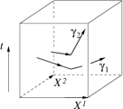
Figure 4: The tunneling processes $A^{(\gamma_{1})}$ and $B^{(\gamma_{2})}$.

Let (see Fig. 4)

$$A^{(\gamma_{1})}=W_{(1,0)}^{(\gamma_{1})},\ \ \ \ \ B^{(\gamma_{1})}=W_{(0,1)}^{(\gamma_{1})}.$$

A combination of two tunneling processes in the $X^{1}$ direction: $A^{(\gamma_{1})}$ and then $A^{(\gamma_{2})}$, induces a transformation $A^{(\gamma_{2})}A^{(\gamma_{1})}$ on the degenerate ground states. A combination of the same two tunneling processes but with a different time order: $A^{(\gamma_{2})}$ and then $A^{(\gamma_{1})}$, induces a transformation $A^{(\gamma_{1})}A^{(\gamma_{2})}$ on the degenerate ground states. We note that the two tunneling paths with different time orders can be deformed into each other smoothly. So they only differ by local perturbations. Due to the topological stability of the degenerate ground statesWen and Niu (1990), local perturbations cannot change the degenerate ground states. Therefore $A^{(\gamma_{1})}$ and $A^{(\gamma_{2})}$ commute, and similarly $B^{(\gamma_{1})}$ and $B^{(\gamma_{2})}$ commute too. We see that $A^{(\gamma)}$’s can be simultaneously diagonalized. Similarly, $B^{(\gamma)}$’s can also be simultaneously diagonalized. Due to the $90^{\circ}$ rotation symmetry, $A^{(\gamma)}$ and $B^{(\gamma)}$ have the same set of eigenvalues. But since $A^{(\gamma)}$ and $B^{(\gamma)}$ in general do not commute, we in general cannot simultaneously diagonalize $A^{(\gamma)}$ and $B^{(\gamma)}$.

The basis $\Phi_{\gamma}=\Phi_{\{n_{\gamma;l+l_{s}}\}}$ described by the occupation distribution $n_{\gamma;l+l_{s}}$ on the orbitals $\phi^{(l)}$ is a natural basis in which $A^{(\gamma_{1})}$ is diagonal. This is because the tunneling process $A^{(\gamma_{1})}$ does not move quasiparticle in the $X^{2}$ direction, and hence does not modify the occupation distribution $n_{\gamma;l+l_{s}}$ on the orbitals $\phi^{(l)}$. On the other hand, $B^{(\gamma_{1})}$ does move quasiparticle in the $X^{2}$ direction and hence shifts the occupation distribution $n_{\gamma;l+l_{s}}$ that characterizes the ground states. Therefore $B^{(\gamma_{1})}$ is not diagonal in the $\Phi_{\gamma}$ basis. In particular, when acted on the state $\Phi_{0}\equiv\Phi_{\{n_{l+l_{s}}\}}$ that corresponds to the trivial quasiparticle, $B^{(\gamma_{1})}$ produces the state $\Phi_{\gamma_{1}}$ that corresponds the quasiparticle $\gamma_{1}$:

$$B^{(\gamma_{1})}\Phi_{0}=b_{\gamma_{1}}\Phi_{\gamma_{1}},$$ (51)

where $b_{\gamma_{1}}$ is a non-zero factor. (Note that $\gamma=0,1,\cdots,N_{q}-1$ where $\gamma=0$ corresponds to the trivial quasiparticle and $N_{q}$ is the number of quasiparticle types.)

IV.5.2 Tensor category structure in quasiparticle tunneling operators

Figure 5: A general quasiparticle tunneling process.

$W^{(\gamma)}_{(n_{1},n_{2})}$ is just a special kind of quasiparticle tunneling. In general, we can create many pairs of quasiparticles, move them around each other, combine and/or split quasiparticles, and then annihilate all of them (see Fig. 4). In addition to the quasiparticle-pair creation process represented by a mapping from no-quasiparticle-particle states to two-quasiparticle-particle states and the quasiparticle-pair annihilation process represented by a mapping from two-quasiparticle-particle states to no-quasiparticle-particle states, the more general tunneling process also contains the quasiparticle splitting process represented by a mapping from one-quasiparticle-particle states to two-quasiparticle-particle states and the quasiparticle fusion process represented by a mapping from two-quasiparticle-particle states to one-quasiparticle-particle states. We will use $W({\cal X})$ to represent the action of the whole tunneling process on the degenerate ground state where ${\cal X}$ represents the tunneling path. $W^{(\gamma_{1})}_{(n_{1},n_{2})}$ discussed above is just a special case of $W({\cal X})$.

Due to the topological stability of the degenerate ground states $W({\cal X})$ can have some very nice algebraic properties. However, in order for $W({\cal X})$ to have the nice algebraic structure we need to choose the operators that represent the quasiparticle-pair creation/annihilation and quasiparticle splitting/fusion processes properly. We conjecture that after making those choices, $W({\cal X})$ can satisfy the following conditions:

$$W({\cal X}_{\text{local}}) \propto 1,$$ (52)

$$W\begin{pmatrix}\includegraphics[height=21.68121pt]{Xi0.eps}\end{pmatrix} =W\begin{pmatrix}\includegraphics[height=21.68121pt]{Xis0.eps}\end{pmatrix},$$

$$W\begin{pmatrix}\includegraphics[scale={0.40}]{Xil0.eps}\end{pmatrix} =d_{i}W\begin{pmatrix}\includegraphics[scale={0.40}]{X0.eps}\end{pmatrix},$$

$$W\begin{pmatrix}\includegraphics[scale={0.40}]{XikljO.eps}\end{pmatrix} =\delta_{ij}W\begin{pmatrix}\includegraphics[scale={0.40}]{XikliO.eps}\end{pmatrix},$$

$$W\begin{pmatrix}\includegraphics[scale={0.40}]{XijklmXO.eps}\end{pmatrix} =\sum_{n=0}^{N_{q}-1}F^{ijm}_{kln}W\begin{pmatrix}\includegraphics[scale={0.40}]{XijklnXO.eps}\end{pmatrix},$$

$$W\begin{pmatrix}\includegraphics[scale={0.35}]{Brd1O.eps}\end{pmatrix} =\sum_{k=0}^{N_{q}-1}\omega^{k}_{ij}W\begin{pmatrix}\includegraphics[scale={0.35}]{Brd2O.eps}\end{pmatrix}$$

$$W\begin{pmatrix}\includegraphics[scale={0.35}]{Brd1pO.eps}\end{pmatrix} =\sum_{k=0}^{N_{q}-1}\omega^{k}_{ij}W\begin{pmatrix}\includegraphics[scale={0.35}]{Brd2O.eps}\end{pmatrix}$$

where $i,j,\cdots=0,1,\cdots,N_{q}-1$ label the $N_{q}$ quasiparticle types and $i=0$ corresponds to the trivial quasiparticle. Note that $N_{q}$ is also the ground state degeneracy on the torus. The shaded areas in eqn. (52) represent other parts of tunneling path. Note that there may be tunneling paths that connect disconnected shaded areas.

Here ${\cal X}_{\text{local}}$ represents a tunneling path which has a compact support (ie there is no path in ${\cal X}_{\text{local}}$ that wraps around the torus). In this case $W({\cal X}_{\text{local}})$ represents local perturbations that cannot mix different degenerate ground states on torus.Wen and Niu (1990) Thus $W({\cal X}_{\text{local}})$ must be proportional to the identity. The second relation in eqn. (52) implies that the tunneling amplitude $W({\cal X})$ only depends on the topology of the tunneling path. A smooth deformation of tunneling path will not change $W({\cal X})$.

Strictly speaking, due to the quasiparticle charge and the external magnetic field, we only have $W\begin{pmatrix}\includegraphics[height=21.68121pt]{Xi0.eps}\end{pmatrix}=\hskip 1.0pt\mathrm{e}^{\hskip 1.0pt\mathrm{i}\hskip 1.0pt\theta}W\begin{pmatrix}\includegraphics[height=21.68121pt]{Xis0.eps}\end{pmatrix}$ where $\theta$ is a path dependent phase. However, we can restrict the tunneling paths to be on a properly designed grid, such as a grid formed by squares. We choose the grid such that each square contains $k$ units of flux quanta where $k$ is an integer that satisfies $kQ_{\gamma}$= integer for any $\gamma$. In this case, $\hskip 1.0pt\mathrm{e}^{\hskip 1.0pt\mathrm{i}\hskip 1.0pt\theta}=1$ for the tunneling paths on the grid. Other relations in eqn. (52) are motivated from tensor category theory.BK ; Levin and Wen (2005); Kitaev (2006)

One may notice that the rules (52) are about planar graphs while the tunneling paths are three dimensional graphs. How can one apply rules of planar graphs to three dimensional graphs? Here we have picked a fixed direction of projection and projected the three dimensional tunneling paths to a two dimensional plane.Levin and Wen (2006) The rules (52) apply to such projected planar graphs. Also, the action of tunneling process can only be properly represented by framed graphs in three dimensions, to take into account the phase factors generated by twisting the quasiparticles. Here we have assumed that there is a way to choose a canonical framing for each tunneling process, such that their projections satisfy eqn. (52).

The coefficients $(d_{i},F^{ijm}_{kln},\omega^{k}_{ij})$ must satisfy the following self consistent relations:Levin and Wen (2005); Kitaev (2006)

$$F^{ijk}_{j^{*}i^{*}0} =\frac{v_{k}}{v_{i}v_{j}}\delta_{ijk}$$

$$F^{ijm}_{kln}=F^{lkm^{*}}_{jin} =F^{jim}_{lkn^{*}}=F^{imj}_{k^{*}nl}\frac{v_{m}v_{n}}{v_{j}v_{l}}$$

$$\sum_{n=0}^{N_{q}-1}F^{mlq}_{kpn}F^{jip}_{mns}F^{jsn}_{lkr} =F^{jip}_{qkr}F^{riq}_{mls}$$

$$\omega^{m}_{js}F^{sl^{*}i}_{kjm^{*}}\omega^{l}_{si}\frac{v_{j}v_{s}}{v_{m}} =\sum_{n=0}^{N}F^{ji^{*}k}_{s^{*}nl^{*}}\omega^{n}_{sk}F^{jl^{*}n}_{ksm^{*}}$$

$$\omega^{j}_{is} =\sum_{k=0}^{N_{q}-1}\omega^{k}_{si^{*}}F^{i^{*}s^{*}k}_{isj*}$$ (53)

Here $i^{*}$ is the antiquasiparticle of $i$, $v_{i}$ is defined by $v_{i}=v_{i^{*}}=\sqrt{d_{i}}$, and $\delta_{ijk}$ is given by

$$\delta_{ijk}=\begin{cases}1,&\text{if $i,j,k$ can fuse into a trivial quasiparticle,}\\ 0,&\text{otherwise}\end{cases}$$

We would like to point out that here we only considered a quasiparticle fusion algebra $\psi_{i}\psi_{j}=\sum_{k}N^{k}_{ij}\psi_{k}$ that has a special property $N^{k}_{ij}=0,1$.

IV.5.3 Implications of tensor category structure

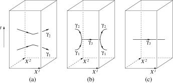
Figure 6: (a): Two tunneling processes: $A^{(\gamma_{1})}$ and $A^{(\gamma_{2})}$. (b): The tunneling path of the above two tunneling processes can be deformed according to the fifth relation in eqn. (52) with $i=\gamma_{2}^{*}$, $j=\gamma_{2}$, $k=\gamma_{1}$, $k=\gamma_{1}^{*}$, $m=0$, and $n=\gamma_{3}$. (c): The fifth, the fourth, and the third relations in eqn. (52) can reduce (b) to (c).

As the first application of the above algebraic structure, we find that (see Fig. 6)

$$A^{(\gamma_{2})}A^{(\gamma_{1})} =\sum_{\gamma_{3}}F^{\gamma_{2}^{*}\gamma_{2}0}_{\gamma_{1}\gamma_{1}^{*}\gamma_{3}}d_{\gamma_{3}}F^{\gamma_{3}\gamma_{1}^{*}\gamma_{2}^{*}}_{\gamma_{2}\gamma_{1}^{*}0}A^{(\gamma_{3})}$$

$$=\sum_{\gamma_{3}}\delta_{\gamma_{1}\gamma_{2}\gamma_{3}^{*}}A^{(\gamma_{3})}.$$ (54)

We see that the algebra of $A^{(\gamma)}$ forms a representation of fusion algebra $\psi_{\gamma_{1}}\psi_{\gamma_{2}}=\sum_{\gamma_{3}}\delta_{\gamma_{1}\gamma_{2}\gamma_{3}^{*}}\psi_{\gamma_{3}}$. The operators $B^{(\gamma)}=SA^{(\gamma)}S^{-1}$ (see eqn. (IV.5.4)) satisfy the same fusion algebra

$$B^{(\gamma_{2})}B^{(\gamma_{1})} =\sum_{\gamma_{3}}\delta_{\gamma_{1}\gamma_{2}\gamma_{3}^{*}}B^{(\gamma_{3})}.$$ (55)

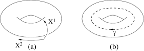
Figure 7: (a): The ground state $\Phi_{\gamma=0}$ on a torus that corresponds to the trivial quasiparticle can be represented by an empty solid torus. (b): The other ground state $\Phi_{\gamma}$ that corresponds to a type $\gamma$ quasiparticle can be represented by an solid torus with a loop of type $\gamma$ in the center.

As the second application of the above algebraic structure, we can represent the degenerate ground states on torus graphically. One of the degenerate ground state $\Phi_{0}$ that corresponds to the trivial quasiparticle $\gamma=0$ can be represented by an empty solid torus (see Fig. 7a). We denote such a state as $|0\rangle=\Phi_{0}$. Other degenerated ground states can be obtained by the action of the $B^{(\gamma)}$ operators

$$|\gamma\rangle\equiv B^{(\gamma)}|0\rangle.$$ (56)

From eqn. (51), we see that $\Phi_{\gamma}$ and $|\gamma\rangle$ are related

$$b_{\gamma}\Phi_{\gamma}=|\gamma\rangle.$$

Since $|\gamma\rangle$ is created by the tunneling operator $B^{(\gamma)}$, $|\gamma\rangle$ can be represented by adding a loop that corresponds to the $B^{(\gamma)}$ operator to the center of the solid torus (see Fig. 7b).

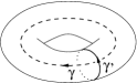
Figure 8: The graphic representation of $A^{(\gamma^{\prime})}|\gamma\rangle$.

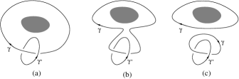
Figure 9: (a): The graphic representation of $A^{(\gamma^{\prime})}|\gamma\rangle$. (b): The graphic representation of $A^{(\gamma^{\prime})}|\gamma\rangle$. (c): The fifth and the fourth relations in eqn. (52) can deformed the graph in (b) to the graph in (c). The shaded area represents the hole of the torus.

$|\gamma\rangle$ is a natural basis for tensor category theory. The matrix elements of $A^{(\gamma)}$ and $B^{(\gamma)}$ have simple forms in such a basis. From eqn. (55), we see that

$$B^{(\gamma_{2})}B^{(\gamma_{1})}|0\rangle =B^{(\gamma_{2})}|\gamma_{1}\rangle=\sum_{\gamma_{3}}\delta_{\gamma_{1}\gamma_{2}\gamma_{3}^{*}}|\gamma_{3}\rangle.$$

Therefore, in the basis $|\gamma\rangle$, the matrix elements of $B^{(\gamma_{2})}$ are given by the coefficients of fusion algebra

$$B^{(\gamma_{2})}_{\gamma_{3}\gamma_{1}}=\delta_{\gamma_{1}\gamma_{2}\gamma_{3}^{*}}.$$ (57)

The action of $A^{(\gamma^{\prime})}$ on $|\gamma\rangle$ is represented by Fig. 8. From Fig. 9, we find that

$$A^{(\gamma^{\prime})}|\gamma\rangle=\frac{S^{\text{TC}}_{\gamma^{*}\gamma^{\prime}}}{d_{\gamma}}|\gamma\rangle,$$ (58)

We see that $A^{(\gamma^{\prime})}$ is diagonal in the $|\gamma\rangle$ basis. Let $a^{(\gamma^{\prime})}_{\gamma}$ be the eigenvalues of $A^{(\gamma^{\prime})}$ we see that

$$a^{(\gamma^{\prime})}_{\gamma}=\frac{S^{\text{TC}}_{\gamma^{*}\gamma^{\prime}}}{d_{\gamma}}=\frac{S^{\text{TC}}_{\gamma^{\prime}\gamma^{*}}}{S^{\text{TC}}_{0\gamma^{*}}}.$$ (59)

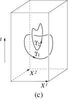
Figure 10: The amplitude of two linked local loops is a complex number $S^{\text{TC}}_{\gamma_{1}\gamma_{2}}$.

$S^{\text{TC}}_{\gamma_{1}\gamma_{2}}$ in eqn. (58) is the amplitude of two linked local loops (see Fig. 10). $S^{\text{TC}}_{\gamma_{1}\gamma_{2}}$ satisfies

$$S^{\text{TC}}_{\gamma_{1}\gamma_{2}}=S^{\text{TC}}_{\gamma_{2}\gamma_{1}}.$$ (60)

Using the tensor category theory (52), one can also show thatKitaev (2006)

$$\frac{S^{\text{TC}}_{\gamma_{1}\gamma}S^{\text{TC}}_{\gamma_{2}\gamma}}{S^{\text{TC}}_{0\gamma}}=\sum_{\gamma_{3}}\delta_{\gamma_{1}\gamma_{2}\gamma^{*}_{3}}S^{\text{TC}}_{\gamma_{3}\gamma}=\sum_{\gamma_{3}}S^{\text{TC}}_{\gamma\gamma_{3}}B^{(\gamma_{1})}_{\gamma_{3}\gamma_{2}}$$ (61)

which can be rewritten as

$$\frac{S^{\text{TC}}_{\gamma_{1}\gamma}}{S^{\text{TC}}_{0\gamma}}\delta_{\gamma\gamma^{\prime}}=\sum_{\gamma_{3}\gamma_{2}}S^{\text{TC}}_{\gamma\gamma_{3}}B^{(\gamma_{1})}_{\gamma_{3}\gamma_{2}}((S^{\text{TC}})^{-1})_{\gamma_{2}\gamma^{\prime}}=A^{(\gamma_{1})}_{\gamma^{*}\gamma^{\prime*}}.$$ (62)

In the operator form, the above becomes

$$A^{(\gamma_{1})}=CS^{\text{TC}}B^{(\gamma_{1})}(S^{\text{TC}})^{-1}C,$$ (63)

where $C$ is the charge conjugation operator $C|\gamma\rangle=|\gamma^{*}\rangle$. We see that $S^{\text{TC}}$ can change the tunneling operator $B^{(\gamma_{1})}$ to $A^{(\gamma_{1})}$. Eqn. (61) can also be rewritten as (assume $S^{\text{TC}}$ is invertible)

$$\sum_{\gamma}\frac{S^{\text{TC}}_{\gamma_{1}\gamma}S^{\text{TC}}_{\gamma_{2}\gamma}((S^{\text{TC}})^{-1})_{\gamma\gamma_{3}}}{S^{\text{TC}}_{0\gamma}}=\delta_{\gamma_{1}\gamma_{2}\gamma^{*}_{3}}$$ (64)

We note that the above expression is invariant under $S^{\text{TC}}_{\gamma^{\prime}\gamma}\to S^{\text{TC}}_{\gamma^{\prime}\gamma}f_{\gamma}$.

$T_{1}$ and $T_{2}$ generate the translation symmetry of the torus. We expect that $T_{1}$ and $T_{2}$ commute with the algebraic structure of the tensor category. Thus we expect that eqn. (IV.4.2) keeps the same form in the new basis $|\gamma\rangle$:

$$T_{1}|\gamma\rangle=\hskip 1.0pt\mathrm{e}^{\hskip 1.0pt\mathrm{i}\hskip 1.0pt2\pi Q_{\gamma}}|\gamma\rangle,\ \ \ \ \ \ \ \ T_{2}|\gamma\rangle=|\gamma^{\prime}\rangle,$$ (65)

where $\gamma^{\prime}$ is the quasiparticle described by the canonical occupation distribution $n_{\gamma^{\prime};l}=n_{\gamma;(l-1)\%m}$.

IV.5.4 Quasiparticle tunneling operators under modular transformation

The transformations $W_{(n_{1},n_{2})}^{(\gamma)}$ induced by quasiparticle tunneling processes have certain algebraic relation with the modular transformations $U(M)$. From Fig. 14, we see that the modular transformation $M_{T}$ changes $W_{(n_{1},n_{2})}^{(\gamma)}$ to $W_{(n_{1}+n_{2},n_{2})}^{(\gamma)}$:

$$TW_{(n_{1},n_{2})}^{(\gamma_{1})} =W_{(n_{1}+n_{2},n_{2})}^{(\gamma_{1})}T.$$ (66)

Since the modular transformation $M_{S}$ generates a $90^{\circ}$ rotation, we find

$$SW_{(n_{1},n_{2})}^{(\gamma_{1})} =W_{(-n_{2},n_{1})}^{(\gamma_{1})}S.$$ (67)

Here $M_{S}$ and $M_{S}$ are given by (47) and $T$ and $S$ are given by (48). Also since the modular transformation $M=-1$ generates a $180^{\circ}$ rotation, we find

$$CW_{(n_{1},n_{2})}^{(\gamma_{1})} =W_{(-n_{2},-n_{1})}^{(\gamma_{1})}C.$$ (68)

In terms of $A^{(\gamma_{1})}$ and $B^{(\gamma_{1})}$ we can rewrite eqn. (66), eqn. (67), and eqn. (68) as

$$TA^{(\gamma_{1})} =A^{(\gamma_{1})}T,$$

$$TB^{(\gamma_{1})} =W_{(1,1)}^{(\gamma_{1})}T,$$

$$SA^{(\gamma_{1})} =B^{(\gamma_{1})}S,$$

$$SB^{(\gamma_{1})}C =CA^{(\gamma_{1})}S,.$$ (69)

Let us assume that the set of the quasiparticle operators $A^{(\gamma)}$ can resolve all the degenerate ground states $|\gamma\rangle$, ie no two degenerate ground states share the common set of eigenvalues for the operators $A^{(\gamma)}$. In this case, the commutation relation $TA^{(\gamma_{1})}=A^{(\gamma_{1})}T$ implies that $T$ is diagonal in the $|\gamma\rangle$ basis. We will fix the over all phase factor of $T$ by choosing $T_{00}=1$.

The operator $C=S^{2}$ is a charge conjugation operator. Its action on $|\gamma\rangle$ is given by (see eqn. (92))

$$C|\gamma\rangle=|\gamma^{*}\rangle.$$

Compare $A^{(\gamma_{1})}=S^{-1}B^{(\gamma_{1})}S=CSB^{(\gamma_{1})}S^{-1}C$ with (63), we find that $S^{\text{TC}}=SF$ where $F$ is a diagonal matrix $F_{\gamma\gamma^{\prime}}=f_{\gamma}\delta_{\gamma\gamma^{\prime}}$ in the $|\gamma\rangle$ basis. Using $S^{\text{TC}}=SF$, we can rewrite eqn. (59) and eqn. (64) as

$$\frac{S_{\gamma_{1}\gamma}f_{\gamma}}{S_{0\gamma}f_{\gamma}}=\frac{S_{\gamma_{1}\gamma}}{S_{0\gamma}}=a^{(\gamma_{1})}_{\gamma^{*}},$$ (70)

$$\sum_{\gamma}\frac{S_{\gamma_{1}\gamma}S_{\gamma_{2}\gamma}(S^{-1})_{\gamma\gamma_{3}}}{S_{0\gamma}}=\delta_{\gamma_{1}\gamma_{2}\gamma^{*}_{3}}$$ (71)

We see that $A^{(\gamma)}$ and $B^{(\gamma)}$ can be determined from $S$.

Since $S^{\text{TC}}$ is symmetric, $S^{\text{TC}}_{0\gamma}=d_{\gamma}>0$ and $S^{\text{TC}}_{00}=1$, once we know $S$, we can use those conditions to fix $F$. Thus we can determine $S^{\text{TC}}$ from $S$. Once we know $S^{\text{TC}}$, we can also calculate the CFT scaling dimension $h_{\gamma}$ for the quasiparticle $\gamma$ (see appendix .6) up to an integer:Kitaev (2006)

$$S^{\text{TC}}_{\gamma_{1}\gamma_{2}}=\sum_{\gamma_{3}}\delta_{\gamma_{1}\gamma_{2}\gamma_{3}^{*}}\hskip 1.0pt\mathrm{e}^{\hskip 1.0pt\mathrm{i}\hskip 1.0pt2\pi(h_{\gamma_{3}}-h_{\gamma_{1}}-h_{\gamma_{2}})}d_{\gamma_{3}}.$$ (72)

The CFT scaling dimensions for the quasiparticles determine the $T$ matrix:

$$T_{\gamma\gamma^{\prime}}=\hskip 1.0pt\mathrm{e}^{\hskip 1.0pt\mathrm{i}\hskip 1.0pt2\pi h_{\gamma}}\delta_{\gamma\gamma^{\prime}}.$$ (73)

IV.6 Summary

In this section, we calculated the charge and the orbital spin of quasiparticle, as well as and the ground state degeneracy from the pattern of zeros $\{S_{a}\}$ of a FQH states. We also discussed the translation transformations, the modular transformations, and the transformations induced by the quasiparticle tunneling on the degenerate ground states. The algebra of those transformation can help us to determine the quasiparticle statistics, quasiparticle quantum dimensions, and fusion algebra of the quasiparticles. In particular, we can use the algebra (IV.4.3) and (50) to determine $S$, and then use eqn. (70), eqn. (71), and eqn. (72) to determine the quasiparticle tunneling operators, $A^{(\gamma)}$ and $B^{(\gamma)}$, and quasiparticle scaling dimensions $h_{\gamma}$. The condition that the matrix elements of $B^{(\gamma)}$ must be non-negative integers put further constraint on $S$.

V Examples

V.1 Quasiparticles in FQH states

In LABEL:WWsymm, many FQH states are characterized and constructed through patterns of zeros. The pattern of zeros in FQH states can be characterized by a $\boldsymbol{S}$-vector $\boldsymbol{S}=(m;S_{2},\cdots,S_{n})$, or a $\boldsymbol{h}$-vector $\boldsymbol{h}=(\frac{m}{n};h^{\text{sc}}_{1},\cdots,h^{\text{sc}}_{n})$, or an occupation distribution $n_{0}\cdots n_{m-1})$. All those data contain information on two important integers $n$ and $m$. $n$ is the number of electrons in one cluster and $m$ determines the filling fraction $\nu=n/m$.

The FQH states constructed in LABEL:WWsymm include the $Z_{n}$ parafermion states $\Phi_{\frac{n}{m};Z_{n}}$ introduced in LABEL:MR9162,RR9984. The patterns of zeros $\{S_{a}\}$ for those $Z_{n}$ parafermion states are obtained. The occupation distributions $\{n_{l}\}$ of those states agree with those obtained in LABEL:SL0604,BKW0608,ABK0875. LABEL:WWsymm also obtained generalized $Z_{n}$ parafermion states $\Phi_{\frac{n}{m};Z_{n}^{(k)}}$ and their patterns of zeros. $\Phi_{\frac{n}{m};Z_{n}^{(k)}}$ has a filling fraction $\nu=n/m$. Many other new FQH states and their patterns of zeros are also obtained in LABEL:WWsymm, such as the $\Phi_{\frac{n}{2n};C_{n}}$ and the $\Phi_{\frac{n}{n};C_{n}/Z_{2}}$ states.

Once we know the pattern of zeros of a FQH state, we can find all the quasiparticle excitations in such a state, by simply finding all $S_{\gamma,a}$ that satisfy (22) and (25) (note that $n_{\gamma;l}$ in (25) are determined from $S_{\gamma;a}$). From the pattern of zeros that characterizes a quasiparticles, we can find many quantum numbers of that quasiparticle. Here we will summarize those results by just listing the number of quasiparticle types in some FQH states. Then, we will give a more detailed discussion for few simple examples.

For the parafermion states $\Phi_{\frac{n}{2};Z_{n}}$ ($m=2$), we find the numbers of quasiparticle types (NOQT) to be

For the parafermion states $\Phi_{\frac{n}{2+2n};Z_{n}}=\Phi_{\frac{n}{2};Z_{n}}\prod_{i<j}(z_{i}-z_{j})^{2}$ ($m=2+2n$), we find

For the generalized parafermion states $\Phi_{\frac{n}{m};Z_{n}^{(k)}}$, we find

where $k$ and $n$ are coprime. For the composite parafermion states $\Phi_{\frac{n_{1}}{m_{1}};Z_{n_{1}}^{(k_{2})}}\Phi_{\frac{n_{2}}{m_{2}};Z_{n_{2}}^{(k_{2})}}$ obtained as products of two parafermion wave functions , we find

where $n_{1}$ and $n_{2}$ are coprime. The filling fractions of the above composite states are $\nu=\frac{n_{1}n_{2}}{m_{1}n_{2}+m_{2}n_{1}}$.

The above results suggest a pattern. For a (generalized) parafermion state $\Phi_{\frac{n}{m};Z_{n}^{(k)}}$, we can express its filling fraction as $\nu=n/m=p/q$ where $p$ and $q$ are coprime. Then the number of quasiparticle types is given by NOQT$=qD(n)$ where $D(2)=3$, $D(3)=2$, $D(4)=5$, $D(5)=3$, $D(6)=7$, $D(7)=4$, $D(8)=9$, $D(9)=5$, and $D(10)=11$; or $D(n)=n+1$ for $n=$ even and $D(n)=\frac{n+1}{2}$ for $n=$ odd. Similarly, For a composite parafermion state $\Phi_{\frac{n_{1}}{m_{1}};Z_{n_{1}}^{(k_{1})}}\Phi_{\frac{n_{2}}{m_{2}};Z_{n_{2}}^{(k_{2})}}$, we can express its filling fraction as $\nu=\frac{n_{1}n_{2}}{m_{1}n_{2}+m_{2}n_{1}}=p/q$ where $p$ and $q$ are coprime. Then the number of quasiparticle types is given by NOQT$=qD(n_{1})D(n_{2})$.

The corresponding CFT of the above (generalized and composite) parafermion states are known. The numbers of the quasiparticle types can also be calculated from the CFT.BW For the generalized parafermion state $\Phi_{\frac{n}{m};Z_{n}^{(k)}}$ the numbers for the quasiparticle types is given byBW

$$NOQT=\frac{1}{\nu}\frac{n(n+1)}{2}=\frac{m}{n}\frac{n(n+1)}{2}=\frac{m(n+1)}{2}.$$

For the composite parafermion state $\prod_{i}\Phi_{\frac{n_{i}}{m_{i}};Z_{n_{i}}^{(k_{i})}}$ the numbers for the quasiparticle types is given byBW

$$NOQT=\frac{1}{\nu}\prod_{i}\frac{n_{i}(n_{i}+1)}{2}.$$

Here we require that $k_{i}$ is not a factor of $n_{i}$ and $n_{1}$, $n_{2}$, $n_{3}$, $\cdots$ have no common factor. The CFT approach gives rise to exactly the same numbers for the quasiparticle types.

For generalized parafermion states $\Phi_{\frac{n}{m};Z_{n}^{(k)}}$ where $n$ and $k$ have a common factor, we have

For more general composite parafermion states $\Phi_{\frac{n_{1}}{m_{1}};Z_{n_{1}}^{(k_{2})}}\Phi_{\frac{n_{2}}{m_{2}};Z_{n_{2}}^{(k_{2})}}$ where $n_{1}$ and $n_{2}$ have a common factor, we have

For the $\nu=1/2$ states $\Phi_{\frac{n}{2n};C_{n}}$, we have

Note that $\Phi_{\frac{5}{10};C_{5}}$ and $\Phi_{\frac{5}{2};Z_{5}}\Phi_{\frac{5}{8};Z_{5}^{(2)}}$ have the same pattern of zeros and may be the same state. For the $\nu=1$ states $\Phi_{\frac{n}{n};C_{n}/Z_{2}}$, we have

Note that $\Phi_{\frac{8}{8};Z_{8}^{(2)}}$, $\Phi_{\frac{4}{4};C_{4}/Z_{2}}$ and $\Phi_{\frac{4}{2};Z_{4}}\Phi_{\frac{4}{2};Z_{4}}$ have the same pattern of zeros and may be the same state.

For those more general and new FQH states, the corresponding CFT are not identified. Even the stability of those FQH states is unclear. If some of those states contain gapless excitations, then the number of quasiparticle types will make no sense for those gapless states. In the following, we will study a few simple examples in more details.

V.2 $\nu=1/2$ Laughlin state

For the $\nu=1/2$ Laughlin state, $n=1$ and its pattern of zeros is characterized by

$$\Phi_{1/2}:\ (m;S_{2},\cdots,S_{n}) =(2;),$$

$$(\frac{m}{n};h^{\text{sc}}_{1},\cdots,h^{\text{sc}}_{n}) =(\frac{2}{1};0),$$

$$n_{0}\cdots n_{m-1} =10$$

Solving (22), we find that there are two types of quasiparticles. Their canonical occupation distributions and other quantum numbers are given by

Thus $T_{1}$, $T_{2}$, and $T$ are given by

$$T_{1}=\begin{pmatrix}1&0\\ 0&-1\end{pmatrix},\ \ \ \ T_{2}=\begin{pmatrix}0&1\\ 1&0\end{pmatrix},\ \ \ \ T=\begin{pmatrix}1&0\\ 0&t_{1}\end{pmatrix}.$$

Since $l_{max}=0$, from (92), we find that the conjugate of $10$ is $\overline{10}=10$ and the conjugate of $01$ is $\overline{01}=01$. Thus $C=1$.

From $TT_{2}=\hskip 1.0pt\mathrm{e}^{\hskip 1.0pt\mathrm{i}\hskip 1.0pt\pi n/m}T_{2}T_{1}T$ (see eqn. (IV.4.3)) we find that $t_{1}=\hskip 1.0pt\mathrm{i}\hskip 1.0pt$. From $ST_{1}=T_{2}S$, we find that $S_{10}=S_{00}$ and $S_{01}=-S_{11}$. From $S^{2}=C=1$, we find that $S_{11}=-S_{00}$, and $S_{00}=\pm\frac{1}{\sqrt{2}}$. Thus

$$S=\frac{1}{\sqrt{2}}\begin{pmatrix}1&1\\ 1&-1\end{pmatrix},\ \ \ \ \ T=\begin{pmatrix}1&0\\ 0&\hskip 1.0pt\mathrm{i}\hskip 1.0pt\end{pmatrix}.$$

The above implies $(ST)^{3}=\hskip 1.0pt\mathrm{e}^{\hskip 1.0pt\mathrm{i}\hskip 1.0pt\pi/4}$. Those modular transformations, $S$ and $T$, agree with those calculated using the Chern-Simons effective theoryWen (1990) and the explicit FQH wave functions.Keski-Vakkuri and Wen (1993) From $T_{11}=\hskip 1.0pt\mathrm{i}\hskip 1.0pt$, we find that the quasiparticle $(n_{\gamma;l})=(01)$ has a scaling dimension $h=1/4$ and a semion statistics.

Let us introduce

$$T_{m}=\hskip 1.0pt\mathrm{e}^{\hskip 1.0pt\mathrm{i}\hskip 1.0pt2\pi/24}T,\ \ \ \ \ S_{m}=S,$$

We find that $T_{m}$ and $S_{m}$ satisfy

$$S_{m}=1,\ \ \ \ (S_{m}T_{m})^{3}=1.$$

Thus $S_{m}$ and $T_{m}$ generate a linear representation of the modular group.

V.3 $Z_{2}$ parafermion state

The $\nu=1$ bosonic Pfaffian stateMoore and Read (1991) is a $Z_{2}$ parafermion state with $n=2$. Its pattern of zeros is described by

$$\Phi_{\frac{2}{2};Z_{2}}:\ (m;S_{2},\cdots,S_{n}) =(2;0),$$

$$(\frac{m}{n};h^{\text{sc}}_{1},\cdots,h^{\text{sc}}_{n}) =(\frac{2}{2};\frac{1}{2},0),$$

$$(n_{0},\cdots,n_{m-1}) =(2,0)$$

Solving (22), we find that there are three types of quasiparticles:

Thus in the $|\gamma\rangle$ basis, $T_{1}$, $T_{2}$ and $T$ are given by

$$T_{1}=\begin{pmatrix}1&0&0\\ 0&1&0\\ 0&0&-1\\ \end{pmatrix},\ \ \ \ T_{2}=\begin{pmatrix}0&1&0\\ 1&0&0\\ 0&0&1\\ \end{pmatrix},\ \ \ \ T=\begin{pmatrix}1&0&0\\ 0&t_{1}&0\\ 0&0&t_{2}\\ \end{pmatrix}.$$

Since $l_{max}=0$, from (92), we find that $\overline{20}=20$, $\overline{02}=02$, and $\overline{11}=11$. Thus $C=1$.

From $TT_{2}=\hskip 1.0pt\mathrm{e}^{\hskip 1.0pt\mathrm{i}\hskip 1.0pt\pi n/m}T_{2}T_{1}T$ (see eqn. (IV.4.3)) we find that $t_{1}=-1$, but $t_{2}$ is undetermined. Using $ST_{1}=T_{2}S$, $ST_{2}=T_{1}S$, $S^{T}=S$, and $S^{2}=1$, we obtain the following possible solutions:

$$S=\frac{1}{2}\begin{pmatrix}1&1&\sqrt{2}x\\ 1&1&-\sqrt{2}x\\ \sqrt{2}/x&-\sqrt{2}/x&0\\ \end{pmatrix}.$$

Those $S$’s satisfy $(ST)^{3}=t_{2}$.

Using the above $S$, we can calculate the fusion coefficients $\delta_{\gamma_{1}\gamma_{2}\gamma_{3}}$ and $B^{(\gamma)}_{\gamma_{1}\gamma_{2}}$ from eqn. (71). We find that $\delta_{220}=\delta_{221}=1/x^{2}$. The condition $\delta_{\gamma\gamma^{*}0}=1$ fixes $x=\pm 1$. Thus we have the following two possible solutions:

$$S_{1}=\frac{1}{2}\begin{pmatrix}1&1&\sqrt{2}\\ 1&1&-\sqrt{2}\\ \sqrt{2}&-\sqrt{2}&0\\ \end{pmatrix},$$

and

$$S_{2}=\frac{1}{2}\begin{pmatrix}1&1&-\sqrt{2}\\ 1&1&\sqrt{2}\\ -\sqrt{2}&\sqrt{2}&0\\ \end{pmatrix}.$$

We note that the above $S$’s are already symmetric. Thus those $S$’s can regarded as $S^{\text{TC}}$.

Now let us calculate $A^{(\gamma)}$ and $B^{(\gamma)}$, $\gamma=0,1,2$ using eqn. (70). For the first solution $S_{1}$ we find that

$$(a^{(\gamma^{\prime})}_{\gamma})=\begin{pmatrix}1&1&\sqrt{2}\\ 1&1&-\sqrt{2}\\ 1&-1&0\\ \end{pmatrix}$$

where $\gamma$ labels rows and $\gamma^{\prime}$ labels columns. We have

$$A^{(0)} =\begin{pmatrix}1&0&0\\ 0&1&0\\ 0&0&1\\ \end{pmatrix},\ \ \ \ \ A^{(1)}=\begin{pmatrix}1&0&0\\ 0&1&0\\ 0&0&-1\\ \end{pmatrix},$$

$$A^{(2)} =\begin{pmatrix}\sqrt{2}&0&0\\ 0&-\sqrt{2}&0\\ 0&0&0\\ \end{pmatrix}.$$

We see that

$$\begin{pmatrix}A^{(0)}A^{(0)}&A^{(0)}A^{(1)}&A^{(0)}A^{(2)}\\ A^{(1)}A^{(0)}&A^{(1)}A^{(1)}&A^{(1)}A^{(2)}\\ A^{(2)}A^{(0)}&A^{(2)}A^{(1)}&A^{(2)}A^{(2)}\\ \end{pmatrix}=\begin{pmatrix}A^{(0)}&A^{(1)}&A^{(2)}\\ A^{(1)}&A^{(0)}&A^{(2)}\\ A^{(2)}&A^{(2)}&A^{(0)}+A^{(1)}\\ \end{pmatrix}.$$

We recover the fusion algebra of the $Z_{2}$ parafermion theory. We also find that

$$B^{(0)} =\begin{pmatrix}1&0&0\\ 0&1&0\\ 0&0&1\\ \end{pmatrix},\ \ \ \ \ B^{(1)}=\begin{pmatrix}0&1&0\\ 1&0&0\\ 0&0&1\\ \end{pmatrix},$$

$$B^{(2)} =\begin{pmatrix}0&0&1\\ 0&0&1\\ 1&1&0\\ \end{pmatrix}.$$

We see that $B^{(\gamma)}$ also encode the fusion algebra

$$\begin{pmatrix}B^{(0)}|0\rangle&B^{(0)}|1\rangle&B^{(0)}|2\rangle\\ B^{(1)}|0\rangle&B^{(1)}|1\rangle&B^{(1)}|2\rangle\\ B^{(2)}|0\rangle&B^{(2)}|1\rangle&B^{(2)}|2\rangle\\ \end{pmatrix}=\begin{pmatrix}|0\rangle&|1\rangle&|2\rangle\\ |1\rangle&|0\rangle&|2\rangle\\ |2\rangle&|2\rangle&|0\rangle+|1\rangle\\ \end{pmatrix},$$

where $|\gamma\rangle$, $\gamma=0,1,2$ are the degenerate ground states.

For the solution $S_{2}$ we have

$$(a^{(\gamma^{\prime})}_{\gamma})=\begin{pmatrix}1&1&-\sqrt{2}\\ 1&1&\sqrt{2}\\ 1&-1&0\\ \end{pmatrix}$$

and

$$A^{(0)} =\begin{pmatrix}1&0&0\\ 0&1&0\\ 0&0&1\\ \end{pmatrix},\ \ \ \ \ A^{(1)}=\begin{pmatrix}1&0&0\\ 0&1&0\\ 0&0&-1\\ \end{pmatrix},$$

$$A^{(2)} =\begin{pmatrix}-\sqrt{2}&0&0\\ 0&\sqrt{2}&0\\ 0&0&0\\ \end{pmatrix}.$$

$B^{(\gamma)}$ remain the same.

The first row of the $S$-matrix are called quantum dimensions of the quasi-particles. For a unitary topological quantum field theory, all quantum dimensions must be positive real numbers, and moreover $\geq 1$. Therefore, the second solution does not give rise to a unitary topological field theory. Based on this reason, we exclude the $S_{2}$ solution.

The $\nu=1$ bosonic $Z_{2}$ parafermion state $\Phi_{\frac{2}{2};Z_{2}}$ has three degenerate ground states on a torus. In the thin torus limit, the three ground states are described by the occupation distributions $20202020\cdots$, $02020202\cdots$, and $11111111\cdots$.

The $\nu=1/2$ fermionic $Z_{2}$ parafermion state $\Phi_{\frac{2}{2};Z_{2}}\prod(z_{i}-z_{j})$ has six degenerate ground states on a torus. In the thin torus limit, the six ground states are also described by the occupation distributions. Those occupation distributions can be obtained from that of $\Phi_{\frac{2}{2};Z_{2}}$ state given above. We note that multiplying the factor $\prod(z_{i}-z_{j})$ increases the space between every neighboring particles in a distribution by one. For example, it changes $11$ to $101$, $101$ to $1001$, $2$ to $11$, $3$ to $111$, etc . It changes the bosonic distribution $202020\cdots$ to a fermionc distribution $110011001100\cdots$, and changes the distribution $111111\cdots$ to $101010101010\cdots$. Including the translated distributions of $110011001100\cdots$ and $101010101010\cdots$, we find that the fermionic $Z_{2}$ parafermion state $\Phi_{\frac{2}{2};Z_{2}}\prod(z_{i}-z_{j})$ has six degenerate ground states described by the distributions

$$110011001100\cdots,$$

$$011001100110\cdots,$$

$$001100110011\cdots,$$

$$100110011001\cdots,$$

$$101010101010\cdots,$$

$$010101010101\cdots.$$

Note that a unit cell contains $m=4$ (or 2) orbitals.

V.4 $Z_{3}$ parafermion state

The $\nu=3/2$ bosonic $Z_{3}$ parafermion state has a pattern of zeros described by

$$\Phi_{\frac{3}{2};Z_{3}}:\ (m;S_{2},\cdots,S_{n}) =(2;0,0),$$

$$(\frac{m}{n};h^{\text{sc}}_{1},\cdots,h^{\text{sc}}_{n}) =(\frac{2}{3};\frac{2}{3},\frac{2}{3},0),$$

$$(n_{0},\cdots,n_{m-1}) =(3,0)$$

Solving (22), we find that there are four types of quasiparticles:

Thus in the $|\gamma\rangle$ basis, $T_{1}$, $T_{2}$ and $T$ are given by

$$T_{1} =\begin{pmatrix}1&0&0&0\\ 0&-1&0&0\\ 0&0&1&0\\ 0&0&0&-1\\ \end{pmatrix},\ \ \ \ T_{2}=\begin{pmatrix}0&1&0&0\\ 1&0&0&0\\ 0&0&0&1\\ 0&0&1&0\\ \end{pmatrix},$$

$$T =\begin{pmatrix}1&0&0&0\\ 0&t_{1}&0&0\\ 0&0&t&0\\ 0&0&0&t_{1}t_{2}\\ \end{pmatrix}.$$

Since $l_{max}=0$, from (92), we find that $\overline{30}=30$, $\overline{03}=03$, $\overline{21}=21$, and $\overline{12}=12$. Thus $C=1$.

From $TT_{2}=\hskip 1.0pt\mathrm{e}^{\hskip 1.0pt\mathrm{i}\hskip 1.0pt\pi n/m}T_{2}T_{1}T$ (see eqn. (IV.4.3)) we find that $t_{1}=-\hskip 1.0pt\mathrm{i}\hskip 1.0pt$ and $t_{2}=t$. Thus

$$T=\begin{pmatrix}1&0&0&0\\ 0&-\hskip 1.0pt\mathrm{i}\hskip 1.0pt&0&0\\ 0&0&t&0\\ 0&0&0&-\hskip 1.0pt\mathrm{i}\hskip 1.0ptt\\ \end{pmatrix}.$$

We can rewrite $T_{1}$, $T_{2}$, and $T$ in direct product form

$$T_{1} =\sigma^{3}\otimes\sigma^{0}, T_{2} =\sigma^{1}\otimes\sigma^{0},$$

$$T =\begin{pmatrix}1&0\\ 0&-\hskip 1.0pt\mathrm{i}\hskip 1.0pt\end{pmatrix}\otimes\begin{pmatrix}1&0\\ 0&t\end{pmatrix}.$$

Using $ST_{1}=T_{2}S$, $ST_{2}=T_{1}S$, and $S^{2}=1$, we find that $S$ must have the following form

$$S =\frac{1}{\sqrt{2}}\begin{pmatrix}1&1\\ 1&-1\end{pmatrix}\otimes\begin{pmatrix}\cos(\theta)&\sin(\theta)\\ \sin(\theta)&-\cos(\theta)\end{pmatrix}.$$

Note that the above $S$ is already symmetric. Thus we can regard the above $S$ as the $S^{\text{TC}}$.

The direct product form of $T_{1}$, $T_{2}$, $T$, and $S$ suggests that the $U(1)$ charge part and the non-Abelian part separate.DFL So let us concentrate on the non-Abelian part

$$\tilde{T}=\begin{pmatrix}1&0\\ 0&t\end{pmatrix},\ \ \ \ \ \tilde{S}=\begin{pmatrix}\cos(\theta)&\sin(\theta)\\ \sin(\theta)&-\cos(\theta)\end{pmatrix}.$$

From $\tilde{S}$, we can calculate $\tilde{A}^{(\gamma)}$ and $\tilde{B}^{(\gamma)}$ [see eqn. (70) and eqn. (IV.5.4)]. All the matrix elements $\tilde{B}^{(\gamma)}$ must be non-negative integers and $(\tilde{S}\tilde{T})^{3}\propto 1$.

One way to satisfy those conditions is to let

$$\tan(\theta)=\frac{1+\sqrt{5}}{2}\equiv\varphi.$$

In this case

$$\tilde{T}=\begin{pmatrix}1&0\\ 0&\hskip 1.0pt\mathrm{e}^{\pm\hskip 1.0pt\mathrm{i}\hskip 1.0pt4\pi/5}\end{pmatrix},\ \ \ \ \ \tilde{S}=\frac{1}{\sqrt{1+\varphi^{2}}}\begin{pmatrix}1&\varphi\\ \varphi&-1\end{pmatrix}.$$ (74)

and

$$\tilde{A}^{(0)} =1, \tilde{A}^{(1)} =\begin{pmatrix}\varphi&0\\ 0&1-\varphi\end{pmatrix},$$

$$\tilde{B}^{(0)} =1, \tilde{B}^{(1)} =\begin{pmatrix}0&1\\ 1&1\end{pmatrix}.$$

Those are the only valid solutions, which are realized by the Fibonacci anyons. The solutions with $d_{1}<0$ are excluded as reasoned at the end of the last section, and one of the them is the non-unitary Yang-Lee model.

Taking $\gamma_{1}=\gamma_{2}=1$ in eqn. (72), we find that

$$-1=\Big{(}\hskip 1.0pt\mathrm{e}^{-\hskip 1.0pt\mathrm{i}\hskip 1.0pt4\pi\tilde{h}_{1}}+\hskip 1.0pt\mathrm{e}^{-\hskip 1.0pt\mathrm{i}\hskip 1.0pt2\pi\tilde{h}_{1}}\varphi\Big{)}$$

or

$$\cos(2\pi\tilde{h}_{1})=-\varphi/2,$$

which gives us

$$\tilde{h}_{1}=\pm 2/5\text{ mod }1.$$

Since $\tilde{h}_{0}=0$, we see that $\hskip 1.0pt\mathrm{e}^{\hskip 1.0pt\mathrm{i}\hskip 1.0pt2\pi\tilde{h}_{\gamma}}$ are the eigenvalues of the $\tilde{T}$ operator (see eqn. (74)). Let us denote the eigenvalues of the $T$ operator as $\hskip 1.0pt\mathrm{e}^{\hskip 1.0pt\mathrm{i}\hskip 1.0pt2\pi h^{T}_{\gamma}}$. We find, for the two choices of $\tilde{h}^{T}_{1}=\pm 2/5$ (see eqn. (74)),

$$n_{\gamma;l}$$

30 0 0

03 3/4 3/4

12 2/5 3/5

21 3/20 7/20

According to CFT (see appendix .6), the scaling dimension of the quasiparticle operators in the $Z_{3}$ parafermion FQH state is $h_{\gamma}=\frac{Q_{\gamma}^{2}}{3}+h^{\text{sc}}_{\gamma}$. For the quasiparticles 30 and 03, $h^{\text{sc}}_{\gamma}=0$ since those are Abelian quasiparticles. For the quasiparticles 12 and 21, $h^{\text{sc}}_{\gamma}=1/15$. Thus $h_{\gamma}=0$, 3/4, 2/5, and 3/20 for the quasiparticles 03, 30,12, and 21 respectively, which exactly agree with $h^{T}_{\gamma}$ for the case of $\tilde{h}^{T}_{1}=2/5$. This example demonstrates a way to calculateRSW quasiparticle scaling dimensions from the pattern of zeros.

The $\nu=3/2$ bosonic $Z_{3}$ parafermion state $\Phi_{\frac{3}{2};Z_{3}}$ has four degenerate ground states on a torus, described by the occupation distributions

$$3030303030\cdots,$$

$$0303030303\cdots,$$

$$2121212121\cdots,$$

$$1212121212\cdots,$$

The $\nu=3/5$ fermionc $Z_{3}$ parafermion state $\Phi_{\frac{3}{2};Z_{3}}\prod(z_{i}-z_{j})$ has 10 degenerate ground states on a torus, described by the occupation distributions

$$1110011100111001110011100\cdots,$$

$$0111001110011100111001110\cdots,$$

$$0011100111001110011100111\cdots,$$

$$1001110011100111001110011\cdots,$$

$$1100111001110011100111001\cdots,$$

$$1101011010110101101011010\cdots,$$

$$0110101101011010110101101\cdots,$$

$$1011010110101101011010110\cdots,$$

$$0101101011010110101101011\cdots,$$

$$1010110101101011010110101\cdots.$$

Note that a unit cell contains $m=5$ orbitals.

VI Conclusions

Through string-net wave functionsFreedman et al. (2004); Levin and Wen (2005), one can show that non-chiral topological orders can be naturally described and classified by tensor category theory. This raises a question: how to describe and classify the chiral topological order in FQH states? The results in LABEL:WWsymm suggest that the pattern of zeros may provide a way to characterize and classify chiral topological orders in FQH states. In this paper, we see that many topological properties of chiral topological orders can be calculated from the data $\{S_{a}\}$ that describe the pattern of zeros. In particular, through the algebra of tunneling operators, we see a close connection to tensor category theory. The pattern of zeros provides a link from electron wave functions (the symmetric polynomials) to tensor category theory and the corresponding chiral topological orders.

Appendix

.1 The calculation of orbital spin

Let

$$F_{L,J}(\alpha) =\sum_{l=0}(l-J)\hskip 1.0pt\mathrm{e}^{-\alpha^{2}l^{2}}\delta_{l\%m-L}$$

$$=\sum_{k=0}(km+L-J)\hskip 1.0pt\mathrm{e}^{-\alpha^{2}(km+L)^{2}}.$$ (75)

We find that, for a canonical occupation distribution (25), we can rewrite (31) as

$$\theta^{\gamma}_{B}=\Omega\sum_{l=0}^{m-1}(n_{\gamma;l}-n_{l})F_{l}(\alpha).$$ (76)

To evaluate $F_{L,J}(\alpha)$, we will use the Euler-Maclaurin formula:

$$\ \ \ \ \frac{f(0)+f(k_{max})}{2}+\sum_{k=1}^{k_{max}}f(k)-\int_{0}^{k_{max}}f(x)\hskip 1.0pt\mathrm{d}x$$

$$=\sum_{k=1}^{p}\frac{B_{k+1}}{(k+1)!}\Big{(}f^{(k)}(k_{max})-f^{(k)}(0)\Big{)}+R,$$

where $B_{k}$ are Bernoulli numbers $(B_{0},B_{1},B_{2},B_{3},\cdots)=(1,-\frac{1}{2},\frac{1}{6},0,-\frac{1}{30},\cdots)$, and

$$|R|\leq\frac{2}{(2\pi)^{2p}}\int_{0}^{n}|f^{(2p+1)}(x)|\hskip 1.0pt\mathrm{d}x.$$

For our case $f(x)=(L+mx-J)\hskip 1.0pt\mathrm{e}^{-\alpha^{2}(mx+L)^{2}}$. If we choose $\alpha\sim 1/J$ and $p=1$, in large $J$ limit, we find $R\sim 1/J$ in large $J$ limit. Therefore

$$\ \ \ \ F_{L,J}(\alpha)$$

$$=\int_{0}^{\infty}(L+mx-J)\hskip 1.0pt\mathrm{e}^{-\alpha^{2}(mx+L)^{2}}\hskip 1.0pt\mathrm{d}x$$

$$\ \ \ \ \ \ \ \ \ \ +\frac{1}{2}(L-J)-\frac{m}{12}+O(1/J)$$

$$=\int_{0}^{\infty}\frac{L+\frac{x}{\alpha}-J}{m\alpha}\hskip 1.0pt\mathrm{e}^{-(x+\alpha L)^{2}}\hskip 1.0pt\mathrm{d}x$$

$$\ \ \ \ \ \ \ \ \ \ +\frac{1}{2}(L-J)-\frac{m}{12}+O(1/J)$$

$$=\int_{0}^{\infty}\frac{L+\frac{x}{\alpha}-J}{m\alpha}(1-2\alpha Lx-\alpha^{2}L^{2}+2\alpha^{2}L^{2}x^{2})\hskip 1.0pt\mathrm{e}^{-x^{2}}\hskip 1.0pt\mathrm{d}x$$

$$\ \ \ \ \ \ \ \ \ \ +\frac{1}{2}(L-J)-\frac{m}{12}+O(1/J)$$

$$=-\frac{\alpha J\sqrt{\pi}-1}{2\alpha^{2}m}+\frac{J}{m}L-\frac{L^{2}}{2m}+\frac{L-J}{2}-\frac{m}{12}+O(1/J).$$

Since $\sum_{l=0}^{m-1}(n_{l}-n_{\gamma;l})=0$ for a canonical occupation distribution, the terms that do not depend on $L$ do not contribute to the Berry’s phase. Thus we have

$$\theta^{\gamma}_{B}=\Omega\sum_{l=0}^{m-1}(n_{\gamma;l}-n_{l})\Big{(}\frac{J}{m}l+\frac{l}{2}-\frac{l^{2}}{2m}\Big{)}.$$ (77)

Compare with (26) and (28), we find that the $\frac{J}{m}l$ term exactly reproduces the quasiparticle charge. The terms that do not depend on $J$ give us the orbital spin (32).

Since $n_{l}$ is a periodic function of $l$ with a period $m$, we may also view $n_{l}$ as a periodic function with a period $km$. If we view $n_{l}$ as a periodic function with a period $km$, the orbital spin $S_{\gamma}^{\text{osp}}$ will be given by

$$S_{\gamma}^{\text{osp}} =\sum_{l=0}^{km-1}(n_{\gamma;l}-n_{l})\Big{(}\frac{l}{2}-\frac{l^{2}}{2km}\Big{)}$$

$$=\sum_{j=0}^{k-1}\sum_{l=0}^{m-1}(n_{\gamma;l}-n_{l})\Big{(}\frac{jm+l}{2}-\frac{(jm+l)^{2}}{2km}\Big{)}$$

$$=\sum_{j=0}^{k-1}\sum_{l=0}^{m-1}(n_{\gamma;l}-n_{l})\Big{(}\frac{l}{2}-\frac{jl}{k}-\frac{l^{2}}{2km}\Big{)}$$

$$=\sum_{l=0}^{m-1}(n_{\gamma;l}-n_{l})\Big{(}\frac{kl}{2}-\frac{k(k-1)l}{2k}-\frac{l^{2}}{2m}\Big{)}$$

$$=\sum_{l=0}^{m-1}(n_{\gamma;l}-n_{l})\Big{(}\frac{l}{2}-\frac{l^{2}}{2m}\Big{)},$$

which is identical to the previous result (32). Therefore, the formal calculation of $S_{\gamma}^{\text{osp}}$ using $\hskip 1.0pt\mathrm{e}^{-\alpha^{2}l^{2}}$ regulator (see (31)) produces a sensible result.

.2 Orbital spin of Abelian quasiparticles

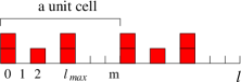
Figure 11: The graphic representation of an occupation distribution $(n_{0},\cdots,n_{10})=(2,0,1,0,2,0,0,0)$ for the $\Phi_{\frac{5}{8};Z_{5}^{(2)}}$ state with $n=5$ and $m=8$. $l_{max}=4$ for such a distribution.

If a quasiparticle is described by an occupation distribution $n_{\gamma;l}$ that can be obtained by shifting the occupation distribution $n_{l}$ for the ground state, then the orbital spin of such a quasiparticle can be calculated reliably without using the formal unreliable approach described above. Such kind of quasiparticles can be created by threading magnetic flux lines through the FQH liquid and correspond to Abelian quasiparticles.

The occupation distribution $n_{l}$ for the ground state has some properties that will be important for the following discussion. In addition to the periodic property $n_{l+m}=n_{l}$, $n_{l}$ also have a symmetric property

$$n_{l}=n_{l_{max}-l},\ \ \ \ \ 0\leq l\leq l_{max}.$$ (78)

according to numerical experiments, where $l_{max}=S_{n}-S_{n-1}$ is the largest $l$ in the first unit cell $0\leq l<m$ such that $n_{l_{max}}>0$ (see Fig. 11). ((78) implies that $n_{0}>0$).

Figure 12: If $N_{\phi}=2J=l_{max}+N_{c}m$, the symmetric polynomial $\Phi$ of $N=N_{c}n$ variables can be put on the sphere without any defects (or quasiparticles).

Figure 13: If $N_{\phi}=2J=l_{max}+(N_{c}-1)m+n_{\phi}$, the above occupation distribution $n_{\gamma;l}$ (obtained by shifting the ground state distribution in Fig. 12) describes a single quasiparticle on the sphere located at the south pole ($l=0$). There is no quasiparticle at the north pole ($l=2J$).

On a sphere with $N_{\phi}=2J$ flux quanta, there are $N_{\phi}+1$ orbitals labeled by $l=0,1,\cdots,2J$ (see Fig. 2). Those orbitals form a angular momentum $J$ representation of the $O(3)$ rotation. The $J_{z}$ quantum numbers of those orbitals are given by $m_{z}=l-J$. If the flux through the sphere is such that $N_{\phi}=2J=l_{max}+(N_{c}-1)m$ for an integer $N_{c}$, then the occupation $n_{l}$ can fit into the $2J+1$ orbital in such a way that there is no non-trivial quasiparticle at the north and south poles (see Fig. (12)). Such a state has $N=N_{c}n$ particles. Such an $N_{c}n$-particle state can fill the sphere without any defect and form a $J^{\text{tot}}=0$ state. Note that $l_{max}=l_{n}=S_{n}-S_{n-1}$ and $S_{n-1}=\frac{n-2}{n}S_{n}$ (see LABEL:WWsymm), thus $l_{max}=\frac{2}{n}S_{n}$. So an $N_{c}n$-particle state can fill the sphere without any defect if $N_{\phi}=2J=\frac{2}{n}S_{n}+(N_{c}-1)m$ which is exactly the condition obtained in LABEL:WWsymm.

Let us create a quasiparticle by threading $n_{\phi}$ flux lines through the south pole. The total flux quanta becomes $N_{\phi}=2J=\frac{2}{n}S_{n}+(N_{c}-1)m+n_{\phi}$ and the occupation distribution $n_{\gamma;l}$ for the created quasiparticle is obtained from $n_{l}$ by shifting the distribution by $n_{\phi}$ (see Fig. 13). The occupation distribution is identical to that of the ground state distribution in Fig. 12 near the north pole ($l=2J$). Thus the distribution describe a state that has no quasiparticle near the north pole. However, the occupation distribution is different from the ground state distribution near the south pole ($l=0$). Therefore, the distribution describes a state with a quasiparticle near the south pole.

The total $J_{z}$ of the above quasiparticle state is given by

$$J^{\text{tot}}_{z} =\sum_{l=0}^{2J}n_{\gamma;l}m_{z}=\sum_{l=0}^{2J}n_{\gamma;l}(l-J)=\frac{n_{\phi}}{2}N$$

$$=\frac{n_{\phi}n}{m}\Big{(}J+\frac{m-l_{max}}{2}-\frac{n_{\phi}}{2}\Big{)}$$

$$=JQ_{\gamma}+\frac{m-l_{max}}{2}Q_{\gamma}-\frac{m}{2n}Q_{\gamma}^{2}$$

where

$$Q_{\gamma}=\frac{n_{\phi}n}{m}$$ (79)

is the quasiparticle charge. If we move such quasiparticle along a loop that spans a solid angle $\Omega$, the induced Berry’s phase $\theta_{B}^{\gamma}$ will be

$$\frac{\theta_{B}^{\gamma}}{\Omega}=J^{\text{tot}}_{z}=JQ_{\gamma}+\frac{m-l_{max}}{2}Q_{\gamma}-\frac{m}{2n}Q_{\gamma}^{2}.$$

Compare with (30), we find the orbital spin of the quasiparticle to be

$$S_{\gamma}^{\text{osp}}=\frac{m-l_{max}}{2}Q_{\gamma}-\frac{m}{2n}Q_{\gamma}^{2}.$$ (80)

Let us compare (80) with (32). For the Abelian quasiparticle, its occupation distribution $n_{\gamma;l}$ has a form

$$n_{\gamma;l}=n_{l-n_{\phi}}.$$

In this case, (32) becomes

$$S_{\gamma}^{\text{osp}} =\sum_{l=0}^{m-1}n_{l}\Big{(}\frac{l+n_{\phi}}{2}-\frac{(l+n_{\phi})^{2}}{2m}-\frac{l}{2}+\frac{l^{2}}{2m}\Big{)}$$

$$=\frac{nn_{\phi}}{2}-\frac{n}{2m}n_{\phi}^{2}-\frac{n_{\phi}}{m}\sum_{l=0}^{m-1}ln_{l}.$$

Using (78), we find that the above expression agrees with (80). This confirms the validity of (32) and (33) for the case of Abelian quasiparticles. On the other hand, the validity of (32) or (33) for the case of non-Abelian quasiparticle is yet to be confirmed by a more rigorous calculation.

.3 Translations of orbitals on torus

To show $T_{2}\phi^{(l)}=\phi^{(l+1)}$, we note that

$$\ \ \ \ T_{2}\phi^{(l)}(X^{1},X^{2})$$

$$=\hskip 1.0pt\mathrm{e}^{\hskip 1.0pt\mathrm{i}\hskip 1.0pt2\pi X^{1}}f^{(l)}\Big{(}X^{1}+\tau(X^{2}+\frac{1}{N_{\phi}})\Big{)}\hskip 1.0pt\mathrm{e}^{\hskip 1.0pt\mathrm{i}\hskip 1.0pt\pi N_{\phi}\tau(X^{2}+\frac{1}{N_{\phi}})^{2}}.$$

Since

$$\ \ f^{(l)}(z+\frac{\tau}{N_{\phi}})=\sum_{k}\hskip 1.0pt\mathrm{e}^{\hskip 1.0pt\mathrm{i}\hskip 1.0pt\frac{\pi\tau}{N_{\phi}}(N_{\phi}k+l)^{2}+\hskip 1.0pt\mathrm{i}\hskip 1.0pt2\pi(N_{\phi}k+l)(z+\frac{\tau}{N_{\phi}})}$$

$$=\hskip 1.0pt\mathrm{e}^{-\hskip 1.0pt\mathrm{i}\hskip 1.0pt\frac{\pi\tau}{N_{\phi}}}\sum_{k}\hskip 1.0pt\mathrm{e}^{\hskip 1.0pt\mathrm{i}\hskip 1.0pt\frac{\pi\tau}{N_{\phi}}(N_{\phi}k+l+1)^{2}+\hskip 1.0pt\mathrm{i}\hskip 1.0pt2\pi(N_{\phi}k+l)z}$$

$$=\hskip 1.0pt\mathrm{e}^{-\hskip 1.0pt\mathrm{i}\hskip 1.0pt\frac{\pi\tau}{N_{\phi}}}\hskip 1.0pt\mathrm{e}^{-\hskip 1.0pt\mathrm{i}\hskip 1.0pt2\pi z}f^{(l+1)}(z),$$

we have

$$\ \ \ \ T_{2}\phi^{(l)}(X^{1},X^{2})$$

$$=\hskip 1.0pt\mathrm{e}^{\hskip 1.0pt\mathrm{i}\hskip 1.0pt2\pi X^{1}-\hskip 1.0pt\mathrm{i}\hskip 1.0pt\frac{\pi\tau}{N_{\phi}}-\hskip 1.0pt\mathrm{i}\hskip 1.0pt2\pi z}f^{(l+1)}(X^{1}+\tau X^{2})\hskip 1.0pt\mathrm{e}^{\hskip 1.0pt\mathrm{i}\hskip 1.0pt\pi N_{\phi}\tau(X^{2}+\frac{1}{N_{\phi}})^{2}}$$

$$=\phi^{(l+1)}(X^{1},X^{2}).$$

.4 Non-Abelian Berry’s phase and modular transformation

The wave functions $\Phi_{\{n_{\gamma;l+l_{s}}\}}$ form a basis of the degenerate ground states. As we change the mass matrix or $\tau$, we obtain a family of basis parameterized by $\tau$. The family of basis can give rise to non-Abelian Berry’s phaseWilczek and Zee (1984) which contain a lot information on topological order in the FQH state. In the following, we will discuss such a non-Abelian Berry’s phase in a general setting. We will use $\gamma$ to label the degenerate ground states.

To find the non-Abelian Berry’s phase, let us first define parallel transportation of a basis. Consider a path $\tau(s)$ that deform the inverse-mass-matrix $g(\tau_{1})$ to $g(\tau_{2})$: $\tau_{1}=\tau(0)$ and $\tau_{2}=\tau(1)$. Assume that for each inverse-mass-matrix $g[\tau(s)]$, the many-electron Hamiltonian on torus $(X^{1},X^{2})\sim(X^{1}+1,X^{2})\sim(X^{1},X^{2}+1)$ has $N_{q}$-fold degenerate ground states $|\gamma;s\rangle$, $\gamma=0,1,\cdots,N_{q}-1$, and a finite energy gap for excitations above the ground states. We can always choose a basis $|\gamma;s\rangle$ for the ground states such that the basis for different $s$ satisfy

$$\langle\gamma^{\prime};s|\frac{\hskip 1.0pt\mathrm{d}}{\hskip 1.0pt\mathrm{d}s}|\gamma;s\rangle=0.$$

Such a choice of basis $|\gamma;s\rangle$ defines a parallel transportation from the bases for inverse-mass-matrix $g(\tau_{1})$ to that for inverse-mass-matrix $g(\tau_{2})$ along the path $\tau(s)$.

In general, the parallel transportation is path dependent. If we choose another path $\tau^{\prime}(s)$ that connect $\tau_{1}$ and $\tau_{2}$, the parallel transportation of the same basis for inverse-mass-matrix $g(\tau_{1})$, $|\gamma;s=0\rangle=|\gamma;s=0\rangle^{\prime}$, may result in a different basis for inverse-mass-matrix $g(\tau_{2})$, $|\gamma;s=1\rangle\neq|\gamma;s=1\rangle^{\prime}$. The different basis are related by an invertible transformation. Such a path dependent invertible transformation is the non-Abelian Berry’s phase.Wilczek and Zee (1984)

However, for the degenerate ground states of a topologically ordered state (including a FQH state), the parallel transportation has a special property that, up to a total phase, it is path independent (in the thermal dynamical limit). The parallel transportations along different paths connecting $\tau_{1}$ and $\tau_{2}$ will change a basis for inverse-mass-matrix $g(\tau_{1})$ to the same basis for inverse-mass-matrix $\tau(\tau_{2})$ up to an overall phase: $|\gamma;s=1\rangle=\hskip 1.0pt\mathrm{e}^{\hskip 1.0pt\mathrm{i}\hskip 1.0pt\phi}|\gamma;s=1\rangle^{\prime}$. In particular, if we deform an inverse-mass-matrix through a loop into itself (ie $\tau(0)=\tau(1)$), the basis $|\gamma;0\rangle$ will parallel transport into $|\gamma;1\rangle=\hskip 1.0pt\mathrm{e}^{\hskip 1.0pt\mathrm{i}\hskip 1.0pt\varphi}|\gamma;0\rangle$. Thus, non-Abelian Berry’s phases for the degenerate states of a topologically ordered state are only path-dependent Abelian phases $\hskip 1.0pt\mathrm{e}^{\hskip 1.0pt\mathrm{i}\hskip 1.0pt\varphi}$ which do not contain much information of topological order.

However, there is a class of special pathes which give rise to non-trivial non-Abelian Berry’s phases. First we note that the torus $(X^{1},X^{2})\sim(X^{1}+1,X^{2})\sim(X^{1},X^{2}+1)$ can be parameterized by another set of coordinates

$$\begin{pmatrix}X^{\prime 1}\\ X^{\prime 2}\\ \end{pmatrix}=\begin{pmatrix}d&-b\\ -c&a\\ \end{pmatrix}\begin{pmatrix}X^{1}\\ X^{2}\\ \end{pmatrix},\ \ \begin{pmatrix}X^{1}\\ X^{2}\\ \end{pmatrix}=\begin{pmatrix}a&b\\ c&d\\ \end{pmatrix}\begin{pmatrix}X^{\prime 1}\\ X^{\prime 2}\\ \end{pmatrix},$$ (81)

where $a,b,c,d\in Z$, $ad-bc=1$. The above can be rewritten in vector form

$$\boldsymbol{X}^{\prime}=M^{-1}\boldsymbol{X},\ \ \ \ \ \ \ \boldsymbol{X}=M\boldsymbol{X}^{\prime},\ \ \ \ M\in SL(2,Z).$$ (82)

$(X^{\prime 1},X^{\prime 2})$ has the same periodicity condition $(X^{\prime 1},X^{\prime 2})\sim(X^{\prime 1}+1,X^{\prime 2})\sim(X^{\prime 1},X^{\prime 2}+1)$ as that for $(X^{1},X^{2})$. We note that

$$\begin{pmatrix}\partial_{X^{1}}\\ \partial_{X^{2}}\\ \end{pmatrix}=\begin{pmatrix}d&-c\\ -b&a\\ \end{pmatrix}\begin{pmatrix}\partial_{X^{\prime 1}}\\ \partial_{X^{\prime 2}}\\ \end{pmatrix},\ \ \ \ \begin{pmatrix}\partial_{X^{\prime 1}}\\ \partial_{X^{\prime 2}}\\ \end{pmatrix}=\begin{pmatrix}a&c\\ b&d\\ \end{pmatrix}\begin{pmatrix}\partial_{X^{1}}\\ \partial_{X^{2}}\\ \end{pmatrix}.$$

The inverse-mass-matrix in the $(X^{1},X^{2})$ coordinate, $g(\tau)$, is changed to

$$g^{\prime}=\begin{pmatrix}d&-b\\ -c&a\\ \end{pmatrix}g(\tau)\begin{pmatrix}d&-c\\ -b&a\\ \end{pmatrix}$$

in the $(X^{\prime 1},X^{\prime 2})$ coordinate. From eqn. (36), we find that

$$g^{\prime}=\begin{pmatrix}\tau_{y}^{\prime}+\frac{{\tau_{x}^{\prime}}^{2}}{\tau_{y}^{\prime}}&-\frac{\tau_{x}^{\prime}}{\tau_{y}^{\prime}}\\ -\frac{\tau_{x}^{\prime}}{\tau_{y}^{\prime}}&\frac{1}{\tau_{y}^{\prime}}\end{pmatrix}=g(\tau^{\prime}),$$ (83)

with

$$\tau^{\prime}=\frac{b+d\tau}{a+c\tau}.$$ (84)

The above transformation $\tau\to\tau^{\prime}$ is the modular transformation. We see that if $\tau$ and $\tau^{\prime}$ are related by the modular transformation, then two inverse-mass-matrices $g(\tau)$ and $g(\tau^{\prime})$ will actually describe the same system (upto a coordinate transformation).

Figure 14: (a): A system described by an inverse-mass-matrix $g(\tau)$. (b): A system described by an inverse-mass-matrix $g(\tau^{\prime})$ where $\tau$ and $\tau^{\prime}$ are related by a modular transformation $M_{T}$. (c): The system in (b) is the same as the system in (a) if we make a change in coordinates. (d): The system in (c) is drawn differently.

Let us assume that the path $\tau(s)$ connects two $\tau$’s related by a modular transformation $M=\begin{pmatrix}a&b\\ c&d\end{pmatrix}$: $\tau(1)=\frac{b+d\tau(0)}{a+c\tau(0)}$. We will denote $\tau(0)=\tau$ and $\tau(1)=\tau^{\prime}$. The parallel transportation of the basis $|\gamma;\tau\rangle$ for inverse-mass-matrix $g[\tau(0)]$ gives us a basis $|\gamma;\tau^{\prime}\rangle$ for inverse-mass-matrix $g[\tau(1)]$. Since $\tau=\tau(0)$ and $\tau^{\prime}=\tau(1)$ are related by a modular transformation, $g[\tau(0)]$ and $g[\tau(1)]$ actually describe the same system. The two basis $|\gamma;\tau\rangle$ and $|\gamma;\tau^{\prime}\rangle$ are actually two basis of same space of the degenerate ground states. Thus there is an invertible matrix that relate the two basis

$$|\gamma;\tau^{\prime}\rangle =U(M)|\gamma;\tau\rangle$$ (85)

$$U_{\gamma\gamma^{\prime}}(M) =\langle\gamma;\tau|\gamma^{\prime};\tau^{\prime}\rangle=\langle\gamma;\tau|U(M)|\gamma^{\prime};\tau\rangle.$$

Such an invertible matrix is the non-Abelian Berry’s phase for the path $\tau(s)$. Except for its overall phase (which is path dependent), the invertible matrix $U$ is a function of the modular transformation $M$. In fact, the invertible matrix $U$ form a projective representation of the modular transformation. The projective representation of the modular transformation contains a lot of information of the underlying topological order.

Let us examine $\langle\gamma;\tau|\gamma^{\prime};\tau\rangle$ in eqn. (85) more carefully. Let $\Phi_{\gamma}[\{\boldsymbol{X}_{i}\}|\tau]$ be ground state wave functions for inverse-mass-matrix $g[\tau]$, and $\Phi_{\gamma}[\{\boldsymbol{X}_{i}\}|\tau^{\prime}]$ be ground state wave functions for inverse-mass-matrix $g[\tau^{\prime}]$. Here $\boldsymbol{X}_{i}=(X^{1}_{i},X^{2}_{i})$ are the coordinates of the $i^{\text{th}}$ electron. Since $\tau$ and $\tau^{\prime}$ are related by a modular transformation, $\Phi_{\gamma}[\{\boldsymbol{X}_{i}\}|\tau]$ and $\Phi_{\gamma}[\{\boldsymbol{X}_{i}\}|\tau^{\prime}]$ are ground state wave function of the same system. However, we cannot directly compare $\Phi_{\gamma}[\{\boldsymbol{X}_{i}\}|\tau]$ and $\Phi_{\gamma}[\{\boldsymbol{X}_{i}\}|\tau^{\prime}]$ and calculate the inner product between the two wave functions as

$$\Big{(}\Phi_{\gamma}[\{\boldsymbol{X}_{i}\}|\tau(0)],\ \Phi_{\gamma^{\prime}}[\{\boldsymbol{X}_{i}\}|\tau^{\prime}]\Big{)}.$$

The wave function $\Phi_{\gamma}[\{\boldsymbol{X}_{i}\}|\tau^{\prime}]$ for inverse-mass-matrix $g[\tau^{\prime}]$ can be viewed as the ground state wave function for inverse-mass-matrix $g[\tau]$ only after a coordinate transformation (see Fig. 14). Let us rename $\boldsymbol{X}$ to $\boldsymbol{X}^{\prime}$ and rewrite $\Phi_{\gamma}[\{\boldsymbol{X}_{i}\}|\tau^{\prime}]$ as $\Phi_{\gamma}(\{\boldsymbol{X}^{\prime}_{i}\}|\tau^{\prime})$. Since the coordinate transformation (82) change $\tau$ to $\tau^{\prime}$, we see that we should really compare $\Phi_{\gamma}(\{\boldsymbol{X}^{\prime}_{i}\}|\tau^{\prime})=\Phi_{\gamma}(\{M^{-1}\boldsymbol{X}_{i}\}|\tau^{\prime})$ with $\Phi_{\gamma}(\{\boldsymbol{X}_{i}\}|\tau)$. But even $\Phi_{\gamma}(\{\boldsymbol{X}_{i}\}|\tau)$ and $\Phi_{\gamma}(\{M^{-1}\boldsymbol{X}_{i}\}|\tau^{\prime})$ cannot be directly compared. This is because the coordinate transformation (81) changes the gauge potential (37) to another gauge equivalent form. We need to perform a $U(1)$ gauge transformation $U_{G}(M)$ to transform the changed gauge potential back to its original form eqn. (37). So only $\Phi_{\gamma}[\{\boldsymbol{X}_{i}\}|\tau]$ and $U_{G}\Phi_{\gamma}[\{M^{-1}\boldsymbol{X}_{i}\}|\tau^{\prime}]$ can be directly compared. Therefore, we have

$$\ \ \ \ U_{\gamma\gamma^{\prime}}(M)$$ (86)

$$=\Big{(}\Phi_{\gamma}(\{\boldsymbol{X}_{i}\}|\tau),U_{G}(M)\Phi_{\gamma^{\prime}}(\{M^{-1}\boldsymbol{X}_{i}\}|\tau^{\prime})\Big{)}$$

which is eqn. (85) in wave function form. Note that $\tau^{\prime}=\frac{M_{12}+M_{22}\tau}{M_{11}+M_{21}\tau}$.

Let us calculate the gauge transformation $U_{G}(M)$. We note that $\Phi_{\gamma}(\{\boldsymbol{X}^{\prime}_{i}\}|\tau^{\prime})$ is the ground state of

$$H^{\prime}=-\sum_{k}\frac{1}{2}\sum_{i,j=1,2}\Big{(}\frac{\partial}{\partial X^{\prime i}_{k}}-\hskip 1.0pt\mathrm{i}\hskip 1.0ptA^{\prime}_{i}\Big{)}g^{\prime}_{ij}\Big{(}\frac{\partial}{\partial X^{\prime j}_{k}}-\hskip 1.0pt\mathrm{i}\hskip 1.0ptA^{\prime}_{j}\Big{)}$$

where $k=1,\cdots,N$ labels the different electrons. In terms of $X^{i}$ (see eqn. (81)), $H^{\prime}$ has a form

$$H^{\prime}=-\sum_{k}\frac{1}{2}\sum_{i,j=1,2}\Big{(}\frac{\partial}{\partial X^{i}_{k}}-\hskip 1.0pt\mathrm{i}\hskip 1.0pt\tilde{A}_{i}\Big{)}g_{ij}\Big{(}\frac{\partial}{\partial X^{j}_{k}}-\hskip 1.0pt\mathrm{i}\hskip 1.0pt\tilde{A}_{j}\Big{)}$$

where

$$\begin{pmatrix}\tilde{A}_{1}\\ \tilde{A}_{2}\\ \end{pmatrix}=\begin{pmatrix}d&-c\\ -b&a\\ \end{pmatrix}\begin{pmatrix}A^{\prime}_{1}\\ A^{\prime}_{2}\\ \end{pmatrix},\ \ \ \ \begin{pmatrix}A^{\prime}_{1}\\ A^{\prime}_{2}\\ \end{pmatrix}=\begin{pmatrix}a&c\\ b&d\\ \end{pmatrix}\begin{pmatrix}\tilde{A}_{1}\\ \tilde{A}_{2}\\ \end{pmatrix}.$$

Since $(A^{\prime}_{1},A^{\prime}_{2})=(-2\pi N_{\phi}X^{\prime 2},0)$, We find that

$$\ \ \ \ (\tilde{A}_{1},\tilde{A}_{2})=(-2\pi N_{\phi}X^{\prime 2}d,\ 2\pi N_{\phi}X^{\prime 2}b)$$

$$=(-2\pi N_{\phi}(-cX^{1}+aX^{2})d,\ 2\pi N_{\phi}(-cX^{1}+aX^{2})b)$$

$U_{G}(M)$ will change $H^{\prime}$ to $H$:

$$\ \ \ \ U_{G}(M)H^{\prime}U_{G}^{\dagger}(M)=H$$

$$=-\sum_{k}\frac{1}{2}\sum_{i,j=1,2}\Big{(}\frac{\partial}{\partial X^{i}_{k}}-\hskip 1.0pt\mathrm{i}\hskip 1.0ptA_{i}\Big{)}g_{ij}\Big{(}\frac{\partial}{\partial X^{j}_{k}}-\hskip 1.0pt\mathrm{i}\hskip 1.0ptA_{j}\Big{)}$$

with $(A_{1},A_{2})=(-2\pi N_{\phi}X^{2},0)$. We find that

$$U_{G}(M) =\prod_{k}u_{G}(M;\boldsymbol{X}_{k}),$$

$$u_{G}(M;\boldsymbol{X}) =\hskip 1.0pt\mathrm{e}^{\hskip 1.0pt\mathrm{i}\hskip 1.0pt2\pi N_{\phi}[bcX^{1}X^{2}-\frac{cd}{2}(X^{1})^{2}-\frac{ab}{2}(X^{2})^{2}]}.$$ (87)

Eqn. (86) can also be rewritten as a transformation on the wave function $\Phi_{\gamma}(\{\boldsymbol{X}_{i}\}|\tau)$:

$$U(M)\Phi_{\gamma}(\{\boldsymbol{X}_{i}\}|\tau) =U_{G}(M)\Phi_{\gamma}(\{\boldsymbol{X}^{\prime}_{i}\}|\tau^{\prime})$$

$$=U_{G}(M)\Phi_{\gamma}(\{M^{-1}\boldsymbol{X}_{i}\}|\tau^{\prime})$$

$$=\Phi_{\gamma^{\prime}}(\{\boldsymbol{X}_{i}\}|\tau)U_{\gamma^{\prime}\gamma}(M).$$ (88)

where $\tau^{\prime}=\frac{M_{12}+M_{22}\tau}{M_{11}+M_{21}\tau}$. We see that the action of the operator $U(M)$ on a wave function $\Phi_{\gamma}(\{\boldsymbol{X}_{i}\}|\tau)$ is to replace $\boldsymbol{X}_{i}$ by $\boldsymbol{X}^{\prime}_{i}=M^{-1}\boldsymbol{X}_{i}$, replace $\tau$ by $\tau^{\prime}=\frac{M_{12}+M_{22}\tau}{M_{11}+M_{21}\tau}$, and then multiply a phase factor $U_{G}(M)$ given in eqn. (.4). Thus eqn. (.4) defines a way how modular transformations act on functions. We find that

$$\ \ \ \ U(M^{\prime})\Big{(}U(M)\Phi_{\gamma}(\{\boldsymbol{X}_{i}\}|\tau)\Big{)}$$

$$=U(M^{\prime})\Big{(}U_{G}(M)\Phi_{\gamma}(\{M^{-1}\boldsymbol{X}_{i}\}|\tau^{\prime})\Big{)}$$

$$=U_{G}(M^{\prime}M)\Phi_{\gamma}(\{M^{-1}M^{\prime-1}\boldsymbol{X}_{i}\}|\tau^{\prime\prime})$$

$$=U_{G}(M^{\prime}M)\Phi_{\gamma}(\{(M^{\prime}M)^{-1}\boldsymbol{X}_{i}\}|\tau^{\prime\prime})$$

$$=U(M^{\prime}M)\Phi_{\gamma}(\{\boldsymbol{X}_{i}\}|\tau).$$

Here $\tau^{\prime}=\frac{M_{12}+M_{22}\tau}{M_{11}+M_{21}\tau}$ and $\tau^{\prime\prime}=\frac{M_{12}+M_{22}\tilde{\tau}}{M_{11}+M_{21}\tilde{\tau}}$ with $\tilde{\tau}=\frac{M^{\prime}_{12}+M^{\prime}_{22}\tau}{M^{\prime}_{11}+M^{\prime}_{21}\tau}$. Thus

$$U(M^{\prime})U(M)=U(M^{\prime}M).$$

So $U(M)$ form a faithful representation of modular transformations $SL(2,Z)$.

To summarize, there are two kinds of deformation loops $\tau(s)$. If $\tau(0)=\tau(1)$, the deformation loop is contractible [ie we can deform the loop to a point, or in other words we can continuously deform the function $\tau(s)$ to a constant function $\tau(s)=\tau(0)=\tau(1)$]. For a contractible loop, the associated non-Abelian Berry’s phase is actually a $U(1)$ phase $U_{\gamma\gamma^{\prime}}=\hskip 1.0pt\mathrm{e}^{\hskip 1.0pt\mathrm{i}\hskip 1.0pt\varphi}\delta_{\gamma\gamma^{\prime}}$. where $\varphi$ is path dependent. If $\tau(0)$ and $\tau(1)$ are related by a modular transformation, the deformation loop is non-contractible. Then the associated non-Abelian Berry’s phase is non-trivial. If two non-contractible loops can be deformed into each other continuously, then the two loops only differ by a contractible loop. The associated non-Abelian Berry’s phases will only differ by an overall $U(1)$ phase. Thus, upto an overall $U(1)$ phase, the non-Abelian Berry’s phases $U_{\gamma\gamma^{\prime}}$ of a topologically ordered state are determined by the modular transformation $\tau\to\tau^{\prime}=\frac{a\tau+b}{c\tau+d}$. We also show that we can use the parallel transportation to defined a system of basis $\Phi_{\gamma}(\{\boldsymbol{X}_{i}\}|\tau)$ for all inverse-mass-matrices labeled by $\tau$. By considering the relation of those basis for two $\tau$’s related by an modular transformation, we can even obtain a faithful representation of the modular transformation $SL(2,Z)$.

.5 Algebra of modular transformations and translations

The translation $T_{\boldsymbol{d}}$ and modular transformation $U(M)$ all act within the space of degenerate ground states. There is an algebraic relation between those operators. From (.4), we see that

$$\ \ \ \ U(M)T_{\boldsymbol{d}}\Phi_{\gamma}(\{\boldsymbol{X}_{i}\}|\tau)=U(M)\Phi_{\gamma}(\{\boldsymbol{X}_{i}+\boldsymbol{d}\}|\tau)$$

$$=U_{G}\Phi_{\gamma}(\{M^{-1}\boldsymbol{X}_{i}+\boldsymbol{d}\}|\tau^{\prime})$$

$$=U_{G}\Phi_{\gamma}(\{M^{-1}(\boldsymbol{X}_{i}+M\boldsymbol{d})\}|\tau^{\prime}).$$

Therefore

$$\hskip 1.0pt\mathrm{e}^{\hskip 1.0pt\mathrm{i}\hskip 1.0pt\theta}U(M)T_{\boldsymbol{d}}=T_{M\boldsymbol{d}}U(M).$$ (89)

Let us determine the possible phase factor $\hskip 1.0pt\mathrm{e}^{\hskip 1.0pt\mathrm{i}\hskip 1.0pt\theta}$ for some special cases. Consider the modular transformation $\tau\to\tau^{\prime}=\tau+1$ generated by

$$M_{T}=\begin{pmatrix}1&1\\ 0&1\end{pmatrix},\ \ \ \ \ M_{T}^{-1}=\begin{pmatrix}1&-1\\ 0&1\end{pmatrix}.$$

We first calculate

$$\ \ \ \ U(M_{T})T_{1}\Phi_{\gamma}(\{\boldsymbol{X}_{i}\}|\tau)=U(M_{T})\Phi_{\gamma}(\{\boldsymbol{X}_{i}+\boldsymbol{d}_{1}\}|\tau)$$

$$=\hskip 1.0pt\mathrm{e}^{-\hskip 1.0pt\mathrm{i}\hskip 1.0pt\pi N_{\phi}\sum_{i}(X_{i}^{2})^{2}}\Phi_{\gamma}(\{M_{T}^{-1}\boldsymbol{X}_{i}+\boldsymbol{d}_{1}\}|\tau^{\prime}).$$

where $\boldsymbol{d}_{1}=(\frac{1}{N_{\phi}},0)$. We note that

$$M_{T}\boldsymbol{d}_{1}=\begin{pmatrix}1&1\\ 0&1\end{pmatrix}\begin{pmatrix}\frac{1}{N_{\phi}}\\ 0\end{pmatrix}=\boldsymbol{d}_{1}.$$

Thus we next calculate

$$\ \ \ \ T_{1}U(M_{T})\Phi_{\gamma}(\{\boldsymbol{X}_{i}\}|\tau)$$

$$=T_{1}\hskip 1.0pt\mathrm{e}^{-\hskip 1.0pt\mathrm{i}\hskip 1.0pt\pi N_{\phi}\sum_{i}(X_{i}^{2})^{2}}\Phi_{\gamma}(\{M_{T}^{-1}\boldsymbol{X}_{i}\}|\tau^{\prime})$$

$$=\hskip 1.0pt\mathrm{e}^{-\hskip 1.0pt\mathrm{i}\hskip 1.0pt\pi N_{\phi}\sum_{i}(X_{i}^{2})^{2}}\Phi_{\gamma}(\{M_{T}^{-1}(\boldsymbol{X}_{i}+\boldsymbol{d}_{1})\}|\tau^{\prime})$$

$$=\hskip 1.0pt\mathrm{e}^{-\hskip 1.0pt\mathrm{i}\hskip 1.0pt\pi N_{\phi}\sum_{i}(X_{i}^{2})^{2}}\Phi_{\gamma}(\{M_{T}^{-1}\boldsymbol{X}_{i}+\boldsymbol{d}_{1}\}|\tau^{\prime}).$$

Therefore

$$U(M_{T})T_{1}=T_{1}U(M_{T}).$$

To obtain the algebra between $U(M_{T})$ and $T_{2}$, we first calculate

$$\ \ \ \ U(M_{T})T_{2}\Phi_{\gamma}(\{\boldsymbol{X}_{i}\}|\tau)$$

$$=U(M_{T})\hskip 1.0pt\mathrm{e}^{\hskip 1.0pt\mathrm{i}\hskip 1.0pt2\pi\sum_{i}X^{1}_{i}}\Phi_{\gamma}(\{\boldsymbol{X}_{i}+\boldsymbol{d}_{2}\}|\tau)$$

$$=\hskip 1.0pt\mathrm{e}^{-\hskip 1.0pt\mathrm{i}\hskip 1.0pt\pi N_{\phi}\sum_{i}(X_{i}^{2})^{2}}\hskip 1.0pt\mathrm{e}^{\hskip 1.0pt\mathrm{i}\hskip 1.0pt2\pi\sum_{i}(X^{1}_{i}-X^{2}_{i})}\Phi_{\gamma}(\{M_{T}^{-1}\boldsymbol{X}_{i}+\boldsymbol{d}_{2}\}|\tau^{\prime}),$$

where $\boldsymbol{d}_{2}=(0,\frac{1}{N_{\phi}})$. We note that

$$M_{T}\boldsymbol{d}_{2}=\begin{pmatrix}1&1\\ 0&1\end{pmatrix}\begin{pmatrix}0\\ \frac{1}{N_{\phi}}\\ \end{pmatrix}=\boldsymbol{d}_{1}+\boldsymbol{d}_{2}.$$

Thus we next calculate

$$\ \ \ \ T_{2}T_{1}U(M_{T})\Phi_{\gamma}(\{\boldsymbol{X}_{i}\}|\tau)$$

$$=T_{2}T_{1}\hskip 1.0pt\mathrm{e}^{-\hskip 1.0pt\mathrm{i}\hskip 1.0pt\pi N_{\phi}\sum_{i}(X_{i}^{2})^{2}}\Phi_{\gamma}(\{M_{T}^{-1}\boldsymbol{X}_{i}\}|\tau^{\prime})$$

$$=T_{2}\hskip 1.0pt\mathrm{e}^{-\hskip 1.0pt\mathrm{i}\hskip 1.0pt\pi N_{\phi}\sum_{i}(X_{i}^{2})^{2}}\Phi_{\gamma}(\{M_{T}^{-1}(\boldsymbol{X}_{i}+\boldsymbol{d}_{1})\}|\tau^{\prime})$$

$$=\hskip 1.0pt\mathrm{e}^{\hskip 1.0pt\mathrm{i}\hskip 1.0pt2\pi\sum_{i}X^{1}_{i}}\hskip 1.0pt\mathrm{e}^{-\hskip 1.0pt\mathrm{i}\hskip 1.0pt\pi N_{\phi}\sum_{i}(X_{i}^{2}+\frac{1}{N_{\phi}})^{2}}\times$$

$$\ \ \ \ \ \ \ \ \ \ \ \Phi_{\gamma}(\{M_{T}^{-1}(\boldsymbol{X}_{i}+\boldsymbol{d}_{1}+\boldsymbol{d}_{2})\}|\tau^{\prime})$$

$$=\hskip 1.0pt\mathrm{e}^{-\hskip 1.0pt\mathrm{i}\hskip 1.0pt\pi N/N_{\phi}}\hskip 1.0pt\mathrm{e}^{\hskip 1.0pt\mathrm{i}\hskip 1.0pt2\pi\sum_{i}(X^{1}-X^{2}_{i})_{i}}\hskip 1.0pt\mathrm{e}^{-\hskip 1.0pt\mathrm{i}\hskip 1.0pt\pi N_{\phi}\sum_{i}(X_{i}^{2})^{2}}\times$$

$$\ \ \ \ \ \ \ \ \ \ \ \Phi_{\gamma}(\{M_{T}^{-1}\boldsymbol{X}_{i}+\boldsymbol{d}_{2})\}|\tau^{\prime}),$$

We see that

$$U(M_{T})T_{2}=\hskip 1.0pt\mathrm{e}^{\hskip 1.0pt\mathrm{i}\hskip 1.0pt\pi\frac{n}{m}}T_{2}T_{1}U(M_{T}).$$

Next we consider the modular transformation $\tau\to\tau^{\prime}=-1/\tau$ generated by

$$M_{S}=\begin{pmatrix}0&-1\\ 1&0\end{pmatrix},\ \ \ \ \ M_{S}^{-1}=\begin{pmatrix}0&1\\ -1&0\end{pmatrix}.$$

From

$$U(M_{S})\Phi_{\gamma}(\{\boldsymbol{X}_{i}\}|\tau) =\hskip 1.0pt\mathrm{e}^{-\hskip 1.0pt\mathrm{i}\hskip 1.0pt2\pi N_{\phi}\sum_{i}X_{i}^{1}X_{i}^{2}}\Phi_{\gamma}(\{M_{S}^{-1}\boldsymbol{X}_{i}\}|\tau^{\prime}),$$

we find

$$\ \ \ \ U(M_{S})U(M_{S})\Phi_{\gamma}(\{\boldsymbol{X}_{i}\}|\tau)$$

$$=U(M_{S})\hskip 1.0pt\mathrm{e}^{-\hskip 1.0pt\mathrm{i}\hskip 1.0pt2\pi N_{\phi}\sum_{i}X_{i}^{1}X_{i}^{2}}\Phi_{\gamma}(\{M_{S}^{-1}\boldsymbol{X}_{i}\}|\tau^{\prime})$$

$$=\hskip 1.0pt\mathrm{e}^{-\hskip 1.0pt\mathrm{i}\hskip 1.0pt2\pi N_{\phi}\sum_{i}X_{i}^{1}X_{i}^{2}}\hskip 1.0pt\mathrm{e}^{-\hskip 1.0pt\mathrm{i}\hskip 1.0pt2\pi N_{\phi}\sum_{i}X_{i}^{2}(-X_{i}^{1})}\Phi_{\gamma}(\{-\boldsymbol{X}_{i}\}|\tau)$$

$$=\Phi_{\gamma}(\{-\boldsymbol{X}_{i}\}|\tau).$$

We see that $U(M_{S})U(M_{S})=U(-1)$ generates to transformation $\boldsymbol{X}\to-\boldsymbol{X}$. We can show that

$$U(-1)T_{1}U^{-1}(-1)=T^{-1}_{1},\ \ \ \ \ \ U(-1)T_{2}U^{-1}(-1)=T^{-1}_{2}.$$ (90)

Since the wave function of an orbital satisfies

$$\phi^{(l)}(-X^{1},-X^{2})=\phi^{(N_{\phi}-l)}(X^{1},X^{2})=\phi^{(-l)}(X^{1},X^{2}),$$

we find

$$U(M_{S})U(M_{S})\Phi_{\gamma}(\{\boldsymbol{X}_{i}\}|\tau) =U(-1)\Phi_{\gamma}(\{\boldsymbol{X}_{i}\}|\tau)$$

$$=\Phi_{\gamma^{*}}(\{\boldsymbol{X}_{i}\}|\tau),$$ (91)

where $\gamma^{*}$ corresponds to the occupation distribution

$$n_{\gamma^{*};l+l_{s}}=n_{\gamma;-l+l_{s}}.$$

Since $n_{\gamma,l}$ and $n_{\gamma^{*},l}$ are periodic with a period of $m$, the above can be rewritten as

$$n_{\gamma^{*};l}=n_{\gamma;(l_{max}-l)\%m}.$$ (92)

$\gamma^{*}$ also corresponds to the anti-quasiparticle of $\gamma$. Thus we find that

$$[U(M_{S})]^{2}=C,\ \ \ \ \ \ C\Phi_{\gamma}=\Phi_{\gamma^{*}},$$

where $C$ is the quasiparticle conjugation operator. Clearly $C^{2}=1$.

Let us first calculate

$$\ \ \ \ U(M_{S})T_{1}\Phi_{\gamma}(\{\boldsymbol{X}_{i}\}|\tau)$$

$$=U(M_{S})\Phi_{\gamma}(\{M_{S}^{-1}\boldsymbol{X}_{i}+\boldsymbol{d}_{1}\}|\tau)$$

$$=\hskip 1.0pt\mathrm{e}^{-\hskip 1.0pt\mathrm{i}\hskip 1.0pt2\pi N_{\phi}\sum_{i}X_{i}^{1}X_{i}^{2}}\Phi_{\gamma}(\{M_{S}^{-1}\boldsymbol{X}_{i}+\boldsymbol{d}_{1}\}|\tau^{\prime}).$$

Since $M_{S}\boldsymbol{d}_{1}=\boldsymbol{d}_{2}$, we next consider

$$\ \ \ \ T_{2}U(M_{S})\Phi_{\gamma}(\{\boldsymbol{X}_{i}\}|\tau)$$

$$=T_{2}\hskip 1.0pt\mathrm{e}^{-\hskip 1.0pt\mathrm{i}\hskip 1.0pt2\pi N_{\phi}\sum_{i}X_{i}^{1}X_{i}^{2}}\Phi_{\gamma}(\{M_{S}^{-1}\boldsymbol{X}_{i}\}|\tau^{\prime})$$

$$=\hskip 1.0pt\mathrm{e}^{\hskip 1.0pt\mathrm{i}\hskip 1.0pt2\pi\sum_{i}X^{1}_{i}}\hskip 1.0pt\mathrm{e}^{-\hskip 1.0pt\mathrm{i}\hskip 1.0pt2\pi N_{\phi}\sum_{i}X_{i}^{1}(X_{i}^{2}+\frac{1}{N_{\phi}})}\times$$

$$\ \ \ \ \ \ \ \ \ \ \ \ \Phi_{\gamma}(\{M_{S}^{-1}(\boldsymbol{X}_{i}+\boldsymbol{d}_{2})\}|\tau^{\prime})$$

$$=\hskip 1.0pt\mathrm{e}^{-\hskip 1.0pt\mathrm{i}\hskip 1.0pt2\pi N_{\phi}\sum_{i}X_{i}^{1}X_{i}^{2}}\Phi_{\gamma}(\{M_{S}^{-1}(\boldsymbol{X}_{i}+\boldsymbol{d}_{2})\}|\tau^{\prime}).$$

We see that

$$U(M_{S})T_{1} =T_{2}U(M_{S}),$$

$$U(M_{S})T_{2} =T^{-1}_{1}U(M_{S}),$$

where we have used (90). Let us introduce

$$T=\hskip 1.0pt\mathrm{e}^{\hskip 1.0pt\mathrm{i}\hskip 1.0pt\theta}U(M_{T}),\ \ \ \ \ \ S=U(M_{S}),$$

where the value of $\theta$ will be chosen to make $T_{00}=1$. We find that

$$TT_{1} =T_{1}T, TT_{2} =\hskip 1.0pt\mathrm{e}^{\hskip 1.0pt\mathrm{i}\hskip 1.0pt\pi\frac{n}{m}}T_{2}T_{1}T,$$

$$ST_{1} =T_{2}S, ST_{2} =CT_{1}C^{-1}S.$$ (93)

.6 Relation to conformal field theory

The symmetric polynomial $\Phi$ can be written as a correlation function of vertex operators $V_{e}(z)$ in a conformal field theory (CFT):Moore and Read (1991); Wen and Wu (1994); Wen et al. (1994)

$$\Phi(\{z_{i}\})=\lim_{z_{\infty}\to\infty}z_{\infty}^{2h_{N}}\langle V(z_{\infty})\prod_{i}V_{e}(z_{i})\rangle$$ (94)

$V_{e}$ (which will be called an electron operator) has a form

$$V_{e}(z)=\psi(z)\hskip 1.0pt\mathrm{e}^{\hskip 1.0pt\mathrm{i}\hskip 1.0pt\phi(z)/\sqrt{\nu}}$$

where $\psi$ is a simple current operator and $\hskip 1.0pt\mathrm{e}^{\hskip 1.0pt\mathrm{i}\hskip 1.0pt\phi(z)/\sqrt{\nu}}$ is the vertex operator on a Gaussian model with a scaling dimension $h=\frac{1}{2\nu}$. The scaling dimension $h^{\text{sc}}_{a}$ of $\psi_{a}(z)\equiv[\psi(z)]^{a}$ has being calculated from the pattern of zeros $\{S_{a}\}$ in LABEL:WWsymm:

$$h^{\text{sc}}_{a}=S_{a}-\frac{aS_{n}}{n}+\frac{am}{2}-\frac{a^{2}m}{2n}.$$ (95)

The quasiparticle state $\Phi_{\gamma}$ can also be expressed as a correlation function in a CFT:

$$\Phi_{\gamma}(\{z_{i}\})=\lim_{z_{\infty}\to\infty}z_{\infty}^{2h^{q}_{N}}\langle V_{q}(z_{\infty})V_{\gamma}(0)\prod_{i}V_{e}(z_{i})\rangle$$ (96)

(Note that $\Phi_{\gamma}$ has a quasiparticle at $z=0$.) Here $V_{\gamma}$ is a quasiparticle operator in CFT which has a form

$$V_{\gamma}(z)=\sigma_{\gamma}(z)\hskip 1.0pt\mathrm{e}^{\hskip 1.0pt\mathrm{i}\hskip 1.0pt\phi(z)Q_{\gamma}/\sqrt{\nu}}$$ (97)

where $\sigma_{\gamma}(z)$ is a “disorder” operator in the CFT generated by the simple current operator $\psi$. Different quasiparticles labeled by different $\gamma$ will correspond to different “disorder” operators.

Let us introduce a quantitative way to characterize the quasiparticle operator. We first fuse the quasiparticle operator with $a$ electron operators:

$$V_{\gamma;a}(z) =V_{\gamma}V_{a}=\sigma_{\gamma;a}(z)\hskip 1.0pt\mathrm{e}^{\hskip 1.0pt\mathrm{i}\hskip 1.0pt\phi(z)Q_{\gamma;a}/\sqrt{\nu}}$$

$$\sigma_{\gamma;a} =\sigma_{\gamma}\psi_{a},\ \ \ \ Q_{\gamma;a}=Q_{\gamma}+a,$$ (98)

where $V_{a}\equiv(V_{e})^{a}=\psi_{a}\hskip 1.0pt\mathrm{e}^{\hskip 1.0pt\mathrm{i}\hskip 1.0pta\phi(z)a/\sqrt{\nu}}$. Then, we consider the operator product expansion (OPE) of $V_{\gamma;a}$ with $V_{e}$

$$V_{e}(z)V_{\gamma;a}(w)=(z-w)^{l^{\text{CFT}}_{\gamma;a+1}}V_{\gamma;a+1}(w).$$ (99)

Let $h_{a}$, $h_{\gamma}$, and $h_{\gamma;a}$ be the scaling dimensions of $V_{a}$, $V_{\gamma}$, and $V_{\gamma;a}$ respectively. We have

$$l^{\text{CFT}}_{\gamma;a+1}=h_{\gamma;a+1}-h_{1}-h_{\gamma;a}.$$ (100)

Since the quasiparticle wave function $\Phi_{\gamma}(\{z_{i}\})$ must be a single valued function of $z_{i}$’s, this requires that $l^{\text{CFT}}_{\gamma;a}$ must be integers. The sequence of integers $\{l^{\text{CFT}}_{\gamma;a}\}$ gives us a quantitative way to characterize quasiparticle operators $V_{\gamma}$ in CFT.

From the occupation distribution description of the quasiparticle $\gamma$ introduced in section III.2, we see that a quasiparticle can also be characterized by another sequence of integers $\{l_{\gamma;a}\}$. What is the relation between the two sequences of integers, $\{l^{\text{CFT}}_{\gamma;a}\}$ and $\{l_{\gamma;a}\}$, that characterize the same set of quasiparticles. From eqn. (99), we see that $l^{\text{CFT}}_{\gamma;a}$ is the order of zeros as we move an electron $z_{i}$ towards a quasiparticle $\gamma$ fused with $a$-electrons. Thus $l^{\text{CFT}}_{\gamma;a}$ is the order of zero $D_{\gamma;a,1}$ introduced in section III.1. From (18) and $S_{1}=0$, we find that $l^{\text{CFT}}_{\gamma;a}$ in the above OPE is given by $l^{\text{CFT}}_{\gamma;a}=S_{\gamma,a}-S_{\gamma,a-1}$. Thus the two sequences, $\{l^{\text{CFT}}_{\gamma;a}\}$ and $\{l_{\gamma;a}\}$, are identical $\{l^{\text{CFT}}_{\gamma;a}\}=\{l_{\gamma;a}\}$. In the rest of the paper, we will drop the superscript CFT in $l^{\text{CFT}}_{\gamma;a}$.

Now let us calculate the quasiparticle charge $Q_{\gamma}$ (see eqn. (97)) from the sequence $\{l_{\gamma;a}\}$ within the CFT. Using $l_{\gamma;a}=S_{\gamma,a}-S_{\gamma,a-1}$, we can rewrite (100) as $h_{\gamma;a+1}-h_{\gamma;a}=S_{\gamma;a+1}-S_{\gamma;a}+h_{1}$. Thus $h_{\gamma;a}-h_{\gamma}=S_{\gamma;a}+ah_{1}$, where we have used $S_{\gamma;0}=S_{\gamma}=0$. Using $h_{1}=h^{\text{sc}}_{1}+\frac{1}{2\nu}=\frac{m}{2}-\frac{S_{n}}{n}$, we find

$$h_{\gamma;a}-h_{\gamma}=S_{\gamma;a}+a\Big{(}\frac{m}{2}-\frac{S_{n}}{n}\Big{)}.$$

Since $\sigma_{\gamma,n}=\sigma_{\gamma}$, we have

$$h_{\gamma;n}-h_{\gamma}=\frac{(Q_{\gamma}+n)^{2}-Q_{\gamma}^{2}}{2\nu}=S_{\gamma;n}+n\Big{(}\frac{m}{2}-\frac{S_{n}}{n}\Big{)}.$$

Thus

$$Q_{\gamma}=\frac{S_{\gamma;n}-S_{n}}{m}=\frac{1}{m}\sum_{a=1}^{n}(l_{\gamma;a}-l_{a}),$$

which agrees with eqn. (27).

Let $h^{\text{sc}}_{\gamma;a}$ be the scaling dimension of $\sigma_{\gamma}\psi_{a}$. We see that $h^{\text{sc}}_{\gamma;a}=h_{\gamma;a}-\frac{(Q_{\gamma}+a)^{2}}{2\nu}$ and

$$h^{\text{sc}}_{\gamma;a}-h^{\text{sc}}_{\gamma}=S_{\gamma;a}-\frac{m}{2n}a^{2}+\Big{(}\frac{m}{2}-\frac{S_{\gamma;n}}{n}\Big{)}a$$

Let

$$s_{\gamma;a}=S_{\gamma;a}-\frac{m}{2n}a^{2}+\Big{(}\frac{m}{2}-\frac{S_{\gamma;n}}{n}\Big{)}a=s_{\gamma;a+n}$$

we can rewrite the above as

$$h^{\text{sc}}_{\gamma;a}=h^{\text{sc}}_{\gamma}+s_{\gamma;a}.$$ (101)

We see that the simple-current part of CFT is determined by $s_{\gamma;a}$, $a=1,\cdots,n-1$, only. In particular, if $\sigma_{\gamma^{\prime}}$ and $\sigma_{\gamma}$ are related by a simple current operator, $\sigma_{\gamma^{\prime}}=\sigma_{\gamma}\psi_{a}$, then the scaling dimension of $\sigma_{\gamma^{\prime}}$ can be calculated from that of $\sigma_{\gamma}$: $h^{\text{sc}}_{\gamma^{\prime}}=h^{\text{sc}}_{\gamma}+s_{\gamma;a}$.

References

- Tsui et al. (1982) D. C. Tsui, H. L. Stormer, and A. C. Gossard, Phys. Rev. Lett. 48, 1559 (1982).
- Laughlin (1983) R. B. Laughlin, Phys. Rev. Lett. 50, 1395 (1983).
- Wen and Niu (1990) X.-G. Wen and Q. Niu, Phys. Rev. B 41, 9377 (1990).
- Wen (1995) X.-G. Wen, Advances in Physics 44, 405 (1995).
- Freedman et al. (2004) M. Freedman, C. Nayak, K. Shtengel, K. Walker, and Z. Wang, Ann. Phys. (NY) 310, 428 (2004).
- Levin and Wen (2005) M. Levin and X.-G. Wen, Phys. Rev. B 71, 045110 (2005).
- Kitaev (2006) A. Kitaev, Annals of Physics 321, 2 (2006).
- (8) B. Bakalov; A. Kirillov, Jr., Lectures on Tensor Categories and Modular Functors, University Lecture Series, vol. 21, Amer. Math. Soc., 2001.
- Kitaev and Preskill (2006) A. Kitaev and J. Preskill, Phys. Rev. Lett. 96, 110404 (2006).
- Levin and Wen (2006) M. Levin and X.-G. Wen, Phys. Rev. Lett. 96, 110405 (2006).
- (11) Xiao-Gang Wen and Zhenghan Wang, arXiv:0801.3291.
- Haldane (1983) F. D. M. Haldane, Phys. Rev. Lett. 51, 605 (1983).
- Greiter et al. (1992) M. Greiter, X.-G. Wen, and F. Wilczek, Nucl. Phys. B 374, 567 (1992).
- Wen (1993) X.-G. Wen, Phys. Rev. Lett. 70, 355 (1993).
- Read and Rezayi (1999) N. Read and E. Rezayi, Phys.Rev. B 59, 8084 (1999).
- Read (2006) N. Read, Phys. Rev. B 73, 245334 (2006).
- Simon et al. (2007) S. H. Simon, E. H. Rezayi, and N. R. Cooper, cond-mat/0701260 (2007).
- Haldane (1985) F. D. M. Haldane, Phys. Rev. Lett. 55, 2095 (1985).
- Wen (1989) X.-G. Wen, Phys. Rev. B 40, 7387 (1989).
- Wen (1990) X.-G. Wen, Int. J. Mod. Phys. B 4, 239 (1990).
- Arovas et al. (1984) D. Arovas, J. R. Schrieffer, and F. Wilczek, Phys. Rev. Lett. 53, 722 (1984).
- Haldane and Rezayi (1985) F. D. M. Haldane and E. H. Rezayi, Phys. Rev. B 31, 2529 (1985).
- Wen (1992) X.-G. Wen, Int. J. Mod. Phys. B 6, 1711 (1992).
- Wen and Zee (1992a) X.-G. Wen and A. Zee, Phys. Rev. Lett. 69, 953 (1992a).
- Wen and Zee (1992b) X.-G. Wen and A. Zee, Phys. Rev. Lett. 69, 3000 (1992b).
- Witten (1989) E. Witten, Comm. Math. Phys. 121, 351 (1989).
- (27) E. Rowell, R. Stong, Z. Wang, arXiv:0712.1377.
- (28) Shiying Dong, Eduardo Fradkin, Robert G. Leigh, and Sean Nowling, arXiv:0802.3231
- Seidel and Lee (2006) A. Seidel and D.-H. Lee, Phys. Rev. Lett. 97, 056804 (2006).
- Bergholtz et al. (2006) E. Bergholtz, J. Kailasvuori, E. Wikberg, T. Hansson, and A. Karlhede, Phys. Rev. B 74, 081308 (2006).
- Seidel and Yang (2008) A. Seidel and K. Yang, arXiv:0801.2402.
- Ardonne et al. (2008) E. Ardonne, E. J. Bergholtz, J. Kailasvuori, and E. Wikberg, arXiv:0802.0675.
- Levin and Wen (2006) M. Levin and X.-G. Wen, Phys. Rev. B 73, 035122 (2006).
- (34) Maissam Barkeshli and Xiao-Gang Wen, to appear.
- Moore and Read (1991) G. Moore and N. Read, Nucl. Phys. B 360, 362 (1991).
- Keski-Vakkuri and Wen (1993) E. Keski-Vakkuri and X.-G. Wen, Int. J. Mod. Phys. B 7, 4227 (1993).
- Wilczek and Zee (1984) F. Wilczek and A. Zee, Phys. Rev. Lett. 52, 2111 (1984).
- Wen and Wu (1994) X.-G. Wen and Y.-S. Wu, Nucl. Phys. B 419, 455 (1994).
- Wen et al. (1994) X.-G. Wen, Y.-S. Wu, and Y. Hatsugai, Nucl. Phys. B 422, 476 (1994).