Modified Kolmogorov Wave Turbulence in QCD matched onto “Bottom-up” Thermalization

Abstract:

We investigate modification of Kolmogorov wave turbulence in QCD calculating gluon spectra as functions of time in the presence of a low energy source which feeds in energy density in the infrared region at a time-dependent rate. Then considering the picture of saturation constraints as has been constructed in the “bottom-up” thermalization approach we revisit that picture for RHIC center-mass energy,  $W=130\,GeV$,  and also extend it to LHC center-mass energy,  $W=5500GeV$,  thus for two cases having an opportunity to calculate the equilibration time,  $\tau_{eq|therm}$,  of the gluon system produced in a central heavy ion collision at mid-rapidity region. Thereby, at RHIC and LHC energies we can match the equilibration time, obtained from the late stage gluon spectrum of the modified Kolmogorov wave turbulence, onto that of the “bottom-up” thermalization and other evolutional approaches as well. In addition, from the revised “bottom-up” approach we find the gluon liberation coefficient to be on the average,  $\varepsilon\simeq 0.81-1.06$  at RHIC and  $\varepsilon\simeq 0.50-0.56$  at LHC. We also present other phenomenological estimates of  $\tau_{therm}$  which, at QCD realistic couplings, yield  $0.45\,fm-0.65\,fm\leq\tau_{therm}\leq 0.97\,fm-2.72\,fm$  at RHIC and  $0.31\,fm-0.40\,fm\leq\tau_{therm}\leq 0.86\,fm-2.04\,fm$  at LHC. We show that the second upper-bounds of  $\tau_{therm}$  in both cases are due to the late stage gluon spectrum of the original Kolmogorov wave turbulence in QCD, previously deduced with a low energy source which feeds in energy density at a constant rate. On the other hand, the lower-bounds and first upper-bounds of  $\tau_{therm}$  are due to the late stage gluon spectrum of the modified QCD wave turbulence, deduced here at the specific time-dependent rate. In the latter case, at certain conditions, taking also into account both very small and realistic couplings we give estimates  $-$   $0.65\,fm\leq\tau_{therm}\leq 1.29\,fm$  at RHIC and  $0.52\,fm\leq\tau_{therm}\leq 1.16\,fm$  at LHC, as well as at realistic couplings we find  $0.53\,<\,\tau_{therm}\,<\,0.7\,fm$  at RHIC and  $0.41\,<\,\tau_{therm}\,<\,0.65\,fm$  at LHC.

1 Introduction

We attempt to continue the investigations which are based on ideas put forward in [1, 2, 3, 4, 5] by Mueller and his colleagues. These articles are devoted to studies of early stages of the gluon system produced in high energy collisions of heavy ions ($AA$) where the main attention is directed to solving the key question of physics of heavy ion collisions: the thermalization of the produced gluon system. In this introductory section we wish to remind the basic results of these and other related studies noting that our ansatz for further proceeding is based on Ref. [5].

Based on the gluon saturation scenario [6, 7], originally, studies of the equilibration picture were performed in [1] where the initial conditions of the produced gluon system are taken from the McLerran-Venugopalan model assuming that all saturated gluons, those having transverse momentum at/or below saturation momentum, $Q_{s}$, in the heavy ion light cone wavefunction, are freed in the high energy collision while the gluons beyond $Q_{s}$ are not freed [8, 9, 10, 11]. Afterwards, the whole discussion was reformulated in a much more general way in terms of the Boltzmann equation [12] with a collision term taken from the elastic gluon-gluon scattering in the one gluon exchange approximation. Here the Boltzmann equation without particle production was considered: the $2\leftrightarrow 2$ process wherein there is a cancellation between gain and loss terms in the elastic collision integral. For this process the time of kinetic equilibration during of which the initial gluon distribution changes significantly is of the order of  $\left(\exp(const/\sqrt{\alpha})\,Q_{s}^{-1}\right)$  which is obtained taking into account a lot of the gluon-gluon elastic scatterings at small angles.

With inclusion of the particle production into the Boltzmann equation the gluon system does seem to approach the kinetic equilibration during a time of the order of  $\left(\sim\,\alpha^{-13/5}Q_{s}^{-1}\right)$  as obtained in [2]. The thermalization occurs in the limit  $Q_{s}\gg\Lambda_{QCD}$  which corresponds to very large nuclei or very high collision energy. The interaction process is described by the “bottom-up” thermalization scenario in $AA$ collisions which is an attempt to study the different stages of evolution of the produced system of the gluons up to the equilibration stage. Furthermore, this scenario provides to some extent agreement with experimental data in respect to hadron multiplicities [3]. However, it was later realized that collective effects in the form of magnetic plasma instabilities, known as Weibel or filamentary instabilities, necessarily play a role in the initial stage of the “bottom-up” equilibration [13] (see [14] and [15] for early discussions as well). Due to the plasma instabilities present in the dense gluon system produced immediately after the collision, the amount of energy transformation, from initially produced hard gluons into softer gluons radiated afterwards by the hard ones, is increased by which one can hope for a rapid thermalization scenario . Nonetheless, it was shown [17] that the full equilibration time in the presence of the instabilities is not much shorter relative to that of the “bottom-up” approach. But the instabilities cannot lead directly to equilibration since they would give an equilibration time parametrically on the order of  $Q_{s}\tau\,\sim\,1$.  For a more detailed insights in this current problem scaling solutions were obtained [4] for pre-equilibrium evolution between the instabilities of the initial stage and the final equilibration. These solutions, depending on one single parameter, match onto the intermediate stage and/or the late stage of the evolution of the gluon system given by the “bottom-up” thermalization which is otherwise called as modified “bottom-up” thermalization (hereafter referred to as m“bottom-up”). Meanwhile, the problems to follow analytically how QCD gluonic system evolves towards the equilibration stage in the presence of the instabilities have not been completely overcome so far (see also [18]). Numerical simulations also seem to indicate that the instabilities are effective at early times. In this regard we hope for further continuous progress of serious numerical studies which can be found in Refs. [16, 19, 20, 21, 22, 23, 24, 25].

Afterwards, the Kolmogorov wave turbulence in QCD (or QCD wave turbulence) was explored in [5] for further better understanding of the instabilities problem in the early stages of the evolution after $AA$ collision, performing calculations for finding time dependences of gluonic spectra, $f_{k}(t)$, in the presence of a low (infrared) energy source which supplies energy at a constant rate to high energetic gluons. In general, the wave turbulence problem [26, 27] (with the low energy source) discussed by Zakharov, L’vov, Falkovich (ZLF) has some generalities with the problem of the instabilities. However, the ZLF and QCD turbulences are somewhat different from each other. In the first case the waves, or particles, interact with each other locally in momentum, e.g., as in a $\Phi^{4}$ theory. But in the second case in QCD the soft and hard gluons have strong interactions along with a lower cutoff in frequency (the so-called plasma frequency which is absent in the $\Phi^{4}$-type theories) or, in other words, the interactions are non-local in momentum modes.

In this paper we attempt to modify the Kolmogorov wave turbulence in QCD. As in [5] the used dynamics stems from the Boltzmann equation with a collision term consisting of  $2\leftrightarrow 2$  and  $2\leftrightarrow 3$  gluon processes. The absence of longrange coherent fields is similarly assumed. Afterwards, the received equilibration time can be matched onto that from various evolutional approaches.

The paper is organized as follows. In the next section we discuss the time stages of the “bottom-up” thermalization and QCD wave turbulence. In the third section we find an early, an intermediate and a late time analytic forms of the gluon spectra in the presence of the low energy source which feeds in energy density at the time-dependent rate  $\dot{\epsilon}_{0}\,=\,\frac{m_{0}^{5}}{\alpha}\,\frac{2}{1+e^{\gamma(\tau/\tau_{0})}}$,  where  $\alpha$  is the QCD coupling constant supposed to be small, $\tau$ is the proper time of the central collision region,  $\tau_{0}=1\,fm$  and  $\gamma$  is a parametric constant the meaning of which will be explained afterwards . For the calculations of the gluon spectra we will follow along the lines of Ref. [5], again supposing that the energy is incoming into our system uniformly in space in the form of the gluons momentum distribution of which are spherically symmetric. These gluons are distributed in phase space uniformly in a range  $m\,<\,\omega\,<\,\bar{m}$  with $m$ to be proportional to the gluon plasma frequency (which defines the soft scale), and $\bar{m}$ on the order of $m$. In the fourth section we calculate the gluon liberation coefficient, $\varepsilon$ (in a limited range), at RHIC and LHC, using the procedure for finding the constraints of the saturation as was done in [3]. Making use of $\varepsilon$ we find a constant factor  $\varepsilon_{eq}$  in the equilibration time formula  $\left(\tau_{eq}\,=\,\varepsilon_{eq}\,\alpha^{-13/5}Q_{s}^{-1}\right)$  of the m“bottom-up”/“bottom-up” thermalization. Thus at RHIC and LHC energies we match the equilibration time, obtained from the late stage gluon spectrum of the modified QCD wave turbulence, onto that of the m“bottom-up”/“bottom-up” thermalization. Then one can see that depending on the value of $\gamma$ and $\alpha$ the matching can occur or not. Finally, in the section fifth we discuss and summarize our results.

2 The time stages of the “bottom-up” thermalization and QCD wave turbulence

2.1 The time stages of the “bottom-up” thermalization

The conventional argument in favor of the thermalization is that at higher collision energy more gluons are freed at a time around $1/Q_{s}$. In the original “bottom-up” picture [2] these gluons (the so-called hard gluons), having momentum at or near the saturation scale of the colliding nuclei, produced after the nuclear impact, lose energy by radiating soft gluons. Hereon, the number of these soft gluons becomes significantly large such that they equilibrate amongst themselves forming a thermal bath which continues to draw energy from the initially produced hard gluons. The full equilibration is achieved when the hard gluons have lost all their energy. The whole process is divided into three distinct stages:

• the early stage  $1\,<\,Q_{s}\tau\,<\,\alpha^{-3/2}$  (the hard gluons dominate);

• the intermediate stage  $\alpha^{-3/2}\,<\,Q_{s}\tau\,<\,\alpha^{-5/2}$  (the hard gluons still dominate in number but the occupation number $f_{h}\,<\,1$);

• the late stage  $\alpha^{-5/2}\,<\,Q_{s}\tau\,<\,\alpha^{-13/5}$  (the soft gluons dominate over the hard ones and the system reaches thermal equilibrium).

But as observed in [13] the early stage of the “bottom-up” is not correct because here instead of having a screening mass (Debye mass, $m_{D}$) the system of the produced hard gluons, having very asymmetrical momentum distribution, leads to a mass characterizing the instabilities. Besides, it is not immediately clear whether at intermediate stage the “bottom-up” is self-consistent. Meanwhile, its late stage part should be consistent since there the Debye mass is determined from the thermalized soft gluons.

However, in the m“bottom-up” thermalization for gluons produced at time $\tau$ there are scaling solutions [4] which allow us interpolate between the instabilities and equilibration. This one-parameter family of the scaling solutions, parametrized by a positive number $\delta$, is the following:

$$N_{s}\,\sim\,\frac{Q_{s}^{3}}{\alpha(Q_{s}\tau)^{4/3-\delta}}\,,\,\,\,\,\,\,\,\,\,\,\,\,\,\,\,k_{s}\,\,\sim\,\,\frac{Q_{s}}{(Q_{s}\tau)^{1/3-2\delta/5}}\,,$$

$$\,\,\,\,\,f_{s}\,\sim\,\frac{1}{\alpha(Q_{s}\tau)^{1/3+\delta/5}}\,,\,\,\,\,\,\,\,\,\,\,\,m_{D}\,\sim\,\frac{Q_{s}}{(Q_{s}\tau)^{1/2-3\delta/10}}\,$$ (1)

where $N_{s}$ is the number density of the soft gluons, $k_{s}$ - the soft gluon momentum, $f_{s}$ - the soft gluon occupation number and the symbol  $\sim$  means that we are still unable to evaluate the total constant factor of each of these expressions. The proposed solutions become identical to the intermediate stage of the “bottom-up” picture in the range  $0\leq\delta\leq 1/3$.  And for the point  $\delta=1/3$  we have the case that the transition from the scaling solutions to the “bottom-up” solution is to the beginning of the late stage of the “bottom-up”, starting at  $Q_{s}\tau\,\sim\,\alpha^{-5/2}$.  When  $\delta>1/3$  the coincidence with the “bottom-up” occurs at the final time $Q_{s}\tau\,\sim\,\alpha^{-13/5}$.

2.2 The time stages of QCD wave turbulence

Now we mention the main conclusions from the recent investigation of QCD wave turbulence [5] in view of the corresponding time stages obtained from the calculations of the gluon spectra as functions of time. Here there are also three distinct stages:

• the early stage  $1\,\ll\,m_{0}\tau\,<\,\alpha^{-7/5}$  (the system is far from the thermal equilibrium and the hard gluons dominate);

• the intermediate stage  $\alpha^{-7/5}\,<\,m_{0}\tau\,<\,\alpha^{-9/5}$  (the gluons having momentum much greater than $m$ are in the thermal equilibrium but the occupation numbers do not coincide with the thermal curve in the domain $m\,<\,\omega\,<\,\bar{m}$);

• the late stage  $m_{0}\tau\,>\,\alpha^{-9/5}$  (the system is very close to the thermal equilibrium where the incoming energy is transferred from the soft scale $m$ to the hard scale given by the temperature $T$ by direct absorption of the soft gluons by the hard gluons in an inelastic $3\rightarrow 2$ process and, parametrically of the same order, by an elastic scattering of the soft gluons on the hard ones with the soft gluons losing energy to them).

We point out that the “bottom-up” thermalization is also based on the observation that both inelastic and elastic processes are equally important for the thermalization [28]. Thus we see that these two approaches have some similarities albeit they are opposite in nature since in QCD wave turbulence we have the energy flow from the soft to hard modes while in the “bottom-up” thermalization we have the energy transformation from the hard into soft modes.

3 The spectrum of the gluons as a function of time and flow weakening parameter

Suppose that at time  $\tau\,=\,0$  we turn on the low energy source of the soft gluons which feeds in the energy density at the rate  $\dot{\epsilon}_{0}\,=\,\frac{m_{0}^{5}}{\alpha}\,\frac{2}{1+e^{\gamma(\tau/\tau_{0})}}$.  Or in other words we conjecture that the energy amount deposited in the soft gauge sector is not a constant in time [5] but instead decreases exponentially with a damping factor, $\gamma$. As noted in the introduction the energy enters into our system isotropically in low momentum modes, nevertheless, as the density of the gluons increases in time the source is modified so that the incoming gluons always have energy just above $m$. Why we take the time-dependent rate for feeding in the energy density will be clear later on when we match the equilibration time from the late stage spectrum onto the equilibration time of the “bottom-up” thermalization.

3.1 The spectrum for   $m_{0}\Psi(\gamma,\tau)>\alpha^{-9/5}$

It is more straightforward to start from the calculation of the late time spectrum and in order to carry out it, first, we keep the dimensions true, namely

$$\dot{\epsilon}(\tau)\,=\,\frac{m_{0}^{5}}{\alpha}\,\frac{2}{1+e^{\gamma(\tau/\tau_{0})}}$$ (1)

where $\gamma$ takes the numbers from $0$ up to $6$: integers and non-integers. The parameter $\gamma$ can also get higher values but we will be restricted up to the number $6$. It describes the degree of the energy flow weakening from the soft to hard scales  .

The energy conservation gives

$$\epsilon(\tau)\,=\,\frac{m_{0}^{5}}{\alpha}\,2\left(\tau-\frac{\tau_{0}}{\gamma}\ln\!\!\left(\frac{1+e^{\gamma(\tau/\tau_{0})}}{2}\right)\right)\,=\,g_{E}T^{4}$$ (2)

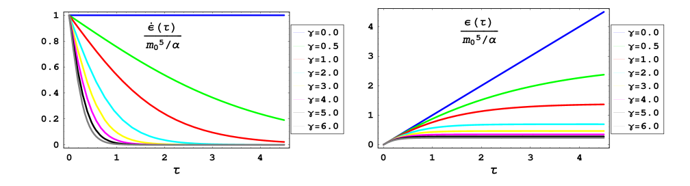
Figure 1: The rate feeding in the energy density (left panel) and the energy density (right panel) as a function of time.

with  $g_{E}\,=\,2(N_{c}^{2}-1)\frac{\pi^{2}}{30}$  (see Fig. 1). Thence

$$T(\tau)\,=\,m_{0}\left[\frac{2\,m_{0}}{g_{E}\,\alpha}\left(\tau-\frac{\tau_{0}}{\gamma}\ln\!\!\left(\frac{1+e^{\gamma(\tau/\tau_{0})}}{2}\right)\right)\right]^{1/4}\,.$$ (3)

We notice that in the limit of $\gamma\,\rightarrow\,0$ we have the case of the study [5]. The soft $m$ and hard $T$ scales are related to each other through  $m\sim\omega_{P}$  where the gluon plasma frequency   $\omega_{P}=m_{\infty}\sqrt{1+\eta\sqrt{4\pi\alpha N_{c}}}$   with   $m_{\infty}=\sqrt{(4\pi/9)N_{c}}\,\sqrt{\alpha}\,T$   [29]. $m_{\infty}$ is also linked to the Debye mass by  $m_{\infty}\,=\,m_{D}/\sqrt{2}$  and the coefficient $\eta$ is equal to  $-0.18$. Nonetheless, for realistic small $\alpha$ the plasma frequency can be approximated as follows:

$$\omega_{P}\,=\,m_{\infty}\sqrt{1+\eta\sqrt{4\pi\alpha N_{c}}}\,\approx\,\sqrt{\frac{4\pi}{9}N_{c}}\,\sqrt{\frac{\alpha}{2.7}}\,\,T\,\,\,\,\,\Rightarrow\,\,\,\,\,m\,\sim\,\sqrt{\alpha}\,T$$ (4)

(at very small $\alpha$’s the denominator $2.7$ in the square root can be replaced by unity).

Consider the elastic scattering of the soft gluons, having momenta $q_{1}$ and $q_{2}$, on the hard gluons, having momenta $p_{1}$ and $p_{2}$ which are of the order of  $T$.  In other words, by this process (see Fig. 2) the soft gluons directly transfer energy to the hard ones.

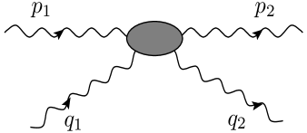
Figure 2: The elastic scattering of the soft and hard gluons. The figure is from [5].

The elastic rate is

$$\dot{\epsilon}^{el} = \frac{[2(N_{c}^{2}-1)]^{2}}{(2\pi)^{12}}\int_{R}\frac{d^{3}p_{1}}{2E_{1}}\frac{d^{3}p_{2}}{2E_{2}}\frac{d^{3}q_{1}}{2\omega_{1}}\frac{d^{3}q_{2}}{2\omega_{2}}\,(2\pi)^{4}\delta^{4}(p_{1}+q_{1}-p_{2}-q_{2})\,|M|^{2}\,\times$$ (5)

$$\times \,[f_{p_{1}}f_{q_{1}}(1+f_{p_{2}})(1+f_{q_{2}})-f_{p_{2}}f_{q_{2}}(1+f_{p_{1}})(1+f_{q_{1}})]\,(\omega_{1}-\omega_{2})$$

where $|M|^{2}$ is the gluon-gluon elastic scattering amplitude

$$|M|^{2}\,=\,\frac{64\pi^{4}}{N_{c}^{2}-1}\left(\frac{\alpha N_{c}}{\pi}\right)^{2}\left(3-\frac{ut}{s^{2}}-\frac{us}{t^{2}}-\frac{ts}{u^{2}}\right)$$ (6)

with

$$s\,=\,(p_{1}+q_{1})^{2}\,,\,\,\,\,\,t\,=\,(q_{1}-q_{2})^{2}\,,\,\,\,\,\,u\,=\,(p_{1}-q_{1})^{2}\,.$$ (7)

The symbol $R$ under the integral sign in Eq. (5) restricts $\omega_{1},\omega_{2}$ to be less than $E_{1},E_{2}$. The magnitudes $\omega_{1}$, $\omega_{2}$, $E_{1}$ and $E_{2}$ are the energies of the soft and hard gluons, respectively.

Let us stress that if the system were in exact equilibrium there would not be flow of the energy and particle number and in that case the spectrum would be given as follows:

$$f_{q_{1},q_{2}}\,=\,\frac{1}{e^{\frac{\omega_{1},\omega_{2}}{T}}-1}\,,\,\,\,\,\,\,\,\,\,\,\,f_{p_{1},p_{2}}\,=\,\frac{1}{e^{\frac{E_{1},E_{2}}{T}}-1}\,,$$ (8)

wherefrom $f_{q}$ can be approximated as

$$f_{q}\,\simeq\,\frac{T}{\omega}$$ (9)

when $\omega/T\ll 1$. Using Eq. (8) for the hard particles we also have

$$1+f_{p}\,=\,f_{p}\,e^{E/T}$$ (10)

which allows us to write the bracket in Eq. (5) as follows (with the use of the energy conservation)

$$[\,\,]\,=\,e^{E_{1}/T}f_{p_{1}}f_{p_{2}}f_{q_{1}}f_{q_{2}}\,[(\omega_{1}-\omega_{2})/T+1/f_{q_{2}}-1/f_{q_{1}}]\,.$$ (11)

The hard momenta are designated as  $p_{i}\,=\,(E_{i},\vec{p}_{i})$  with  $E_{i}\,\approx\,|\vec{p}_{i}|$  while the soft momenta read  $q_{j}\,=\,(\omega_{j},\vec{q}_{j})$  with  $\omega_{j}^{2}\,=\,m^{2}+\vec{q}_{j}^{\,2}\,\approx\,m^{2}$.  The dominant contribution to $|M|^{2}$ comes from the small-$t$ region where  $u\,\approx\,-s$,  so that Eq. (6) switches over to the form

$$|M|^{2}\,\sim\,\alpha^{2}\frac{(E\omega)^{2}}{m^{4}}$$ (12)

where  $(\omega_{1}-\omega_{2})$  is taken to be positive. Taking also

$$d^{3}p_{1}\,\sim\,T^{3}\,,\,\,\,\,\,d^{3}q_{1}\,\sim\,m^{3}\,,\,\,\,\,\,q_{2}^{2}\,\sim\,m^{2}$$ (13)

and doing an integration over $d^{3}p_{2}$ using  $d^{3}q_{2}\,=\,q_{2}^{2}\,dq_{2}\,d\Omega_{q_{2}}$  along with Eq. (4), Eq. (11), Eq. (12) and Eq. (13), one will get that the expression in Eq. (5) takes the form

$$\dot{\epsilon}^{el}\,\sim\,\frac{m_{0}^{5}}{\alpha}\left(\frac{m}{m_{0}}\right)^{5}(\alpha f_{q_{1}})(\alpha f_{q_{2}})[(\omega_{1}-\omega_{2})+T/f_{q_{2}}-T/f_{q_{1}}]\frac{1}{m}\,.$$ (14)

From Eq. (3) and Eq. (4) we have

$$\frac{m}{m_{0}}\,\sim\,\left[2\,\alpha\,m_{0}\left(\tau-\frac{\tau_{0}}{\gamma}\ln\!\!\left(\frac{1+e^{\gamma(\tau/\tau_{0})}}{2}\right)\right)\right]^{1/4}\,.$$ (15)

As well as from Eq. (9) and Eq. (4) one obtains

$$\alpha f_{q}\,\sim\,\alpha T/\omega\,\sim\,\sqrt{\alpha}\,.$$ (16)

Thus

$$\dot{\epsilon}^{el}\,\sim\,\frac{m_{0}^{5}}{\alpha}\frac{2}{1+e^{\gamma(\tau/\tau_{0})}}\,\alpha^{9/4}\left[m_{0}\Psi(\gamma,\tau)\right]^{5/4}[(\omega_{1}-\omega_{2})+T/f_{q_{2}}-T/f_{q_{1}}]\,\frac{1}{m}$$ (17)

where

$$\Psi(\gamma,\tau)\,\equiv\,2\,{\Large{\left(\frac{1+e^{\gamma(\tau/\tau_{0})}}{2}\right)^{4/5}}}\!\left(\tau-\frac{\tau_{0}}{\gamma}\ln\!\!\left(\frac{1+e^{\gamma(\tau/\tau_{0})}}{2}\right)\right)\,.$$ (18)

If $f_{q_{1}}$ and $f_{q_{2}}$ were take the form of Eq. (9) then we would obtain zero in the r.h.s. of Eq. (17). But the incoming flux of the soft gluons increases $f_{q}$ a little, so that the expression  $[(\omega_{1}-\omega_{2})+T/f_{q_{2}}-T/f_{q_{1}}]$  is greater than zero. However, from Eq. (17) it is obvious that by the time  $m_{0}\Psi(\gamma,\tau)\gg\alpha^{-9/5}$,  $f_{q}$ will be very close to the thermal equilibrium distribution making the  $[\,\,]\frac{1}{m}$  small and compensating the expression  $\alpha^{9/4}[m_{0}\Psi(\gamma,\tau)]^{5/4}\,.$

Thus the energy is directly transferred from the incoming gluons of the source to the gluons having the momentum $p\,\sim\,T$. Meanwhile, there is also an interaction with gluons having a momentum $k$ which is greater than the soft scale $m$ and less than the hard scale $T$, but the flow from the source to the $k$-particles is suppressed by a factor $k/T$ compared to the flow to the $T$-particles, so that by this way only a small fraction of the energy is transferred.

Consider the inelastic $3\,\leftrightarrow\,2$ scattering process (see Fig. 3) which is shown to be parametrically equally important as the elastic scattering. By this process the energy is also transferred from the scale $m$ to the scale $T$. The inelastic rate is

$$\dot{\epsilon}^{inel} = 2\,\frac{[2(N_{c}^{2}-1)]^{2}}{(2\pi)^{15}}\int_{R}\frac{d^{3}p_{1}}{2E_{1}}\frac{d^{3}p_{2}}{2E_{2}}\frac{d^{3}p_{3}}{2E_{3}}\frac{d^{3}p_{4}}{2E_{4}}\frac{d^{3}k}{2E_{k}}\,(2\pi)^{4}\delta^{4}(p_{1}+p_{2}+k-p_{3}-p_{4})\,|M_{12k\rightarrow 34}|^{2}\,\times$$ (19)

$$\times \,[f_{p_{1}}f_{p_{2}}f_{k}(1+f_{p_{3}})(1+f_{p_{4}})-f_{p_{3}}f_{p_{4}}(1+f_{p_{1}})(1+f_{p_{2}})(1+f_{k})]\,\omega\,.$$

Figure 3: $3\,\leftrightarrow\,2$ inelastic scattering process. The figure is from [5].

For a detailed calculation of this integral we refer to Ref. [30] as well. Here we put down the final result

$$\dot{\epsilon}^{inel}\,\sim\,\alpha^{3}\frac{T^{6}}{m^{2}}\,[f_{p_{1}}f_{p_{2}}f_{k}(1+f_{p_{3}})(1+f_{p_{4}})-f_{p_{3}}f_{p_{4}}(1+f_{p_{1}})(1+f_{p_{2}})(1+f_{k})]\,\omega\,.$$ (20)

Using Eq. (4), Eq. (9), Eq. (10) and Eq. (15) one can rewrite Eq. (20) as

$$\dot{\epsilon}^{inel}\sim\frac{m_{0}^{5}}{\alpha}\frac{2}{1+e^{\gamma(\tau/\tau_{0})}}\,\alpha^{9/4}\left[m_{0}\Psi(\gamma,\tau)\right]^{5/4}[\omega-T/f_{k}]\,\frac{1}{m}\,.$$ (21)

It is clear that this equation is parametrically equivalent to Eq. (17).

3.2 The spectrum for   $\alpha^{-7/5}\,<\,m_{0}\Psi(\gamma,\tau)\,<\,\alpha^{-9/5}$

From Eq. (17) one clarifies that so long as  $m_{0}\Psi(\gamma,\tau)\,<\,\alpha^{-9/5}$  it is impossible to transfer the energy fast enough from the source in the region  $m\,<\,\omega\,<\,\bar{m}$  to the momentum region close to the scale $T$ if we use a near equilibrium distribution in the soft region. In this scenario the gluons from the source “pile up” in the region  $m\,<\,\omega\,<\,\bar{m}$  whereby the occupation number becomes large enough speeding up the rate of the energy transfer from the scale $m$ to the scale $T$ such that the transfer can compensate the energy rate incoming from the source.

When $\omega\,>\,\bar{m}$ the distribution of the gluons is near to the equilibrium distribution of Eq. (8), nevertheless, when $m\,<\,\omega\,<\,\bar{m}$ the distribution will be noticeably changed (see Fig. 4). Consider gluons having high momenta but located in the region $m\,<\,\omega\,<\,\bar{m}$. They will elastically scatter with the gluons of momentum on the order of $T$ and will lose the energy to the harder gluons as given by Eq. (14) which means that a gluon at the point 1 will move to the point 3 increasing $f_{k_{3}}$. As regards $f_{k_{1}}$, it is determined by the difference between the incoming gluons causing $f_{k_{1}}$ to increase and the scattering on the hard gluons causing $f_{k_{1}}$ to decrease. Therefore, with decrease of $k$ the occupation number $f_{k}$ will increase rapidly until it becomes large enough such that the gluons of the momentum $k$ are absorbed by the hard ones at the same rate which is determined by the emission of the external source and by gluons which acquire the momentum $k$ after elastic scattering on the hard gluons. The estimates of these rates are given below.

Figure 4: The gluon distribution as a function of the energy. The figure is from [5].

The case of the constant inflow of the energy,  $\,\dot{\epsilon}\,=\,m_{0}^{5}/\alpha\,$,  corresponds to an increase in the occupation number,  $\,\dot{f}_{k}\,\sim\,\frac{m}{\alpha}\left(\frac{m_{0}}{m}\right)^{5}$. More precisely it comes from

$$\dot{\epsilon}\,\equiv\,\left(2(N_{c}^{2}-1)\int\frac{d^{3}k}{(2\pi)^{3}}\,\dot{f}_{k}\right)\omega\,\,.$$ (22)

To the time-dependent inflow of the energy, i.e.,  $\dot{\epsilon}\,=\,\frac{m_{0}^{5}}{\alpha}\,\frac{2}{1+e^{\gamma(\tau/\tau_{0})}}$ ,  corresponds the increase in the occupation number,  $\,\dot{f}_{k}\,\sim\,\frac{m}{\alpha}\left(\frac{m_{0}}{m}\right)^{5}\!\!\frac{2}{1+e^{\gamma(\tau/\tau_{0})}}$ .

If we assume $k_{3}$ to be the momentum (see point 3 in Fig. 4) at which the loss by the inelastic absorption exactly balances the rate of the incoming gluons directly from the source or coming from the source via higher momentum regions then the incoming gluons rate will be

$$\dot{f}^{source}_{k_{3}}\,\sim\,\frac{1}{m^{4}}\frac{m_{0}^{5}}{\alpha}\frac{2}{1+e^{\gamma(\tau/\tau_{0})}}\left(\frac{m}{k_{3}}\right)^{3}$$ (23)

where  $\frac{1}{m^{4}}\frac{m_{0}^{5}}{\alpha}\frac{2}{1+e^{\gamma(\tau/\tau_{0})}}$  is the rate of the total number of the incoming gluons arriving over the whole phase space  $m\,<\,\omega\,<\,\bar{m}$. The term  $\left(\frac{m}{k_{3}}\right)^{3}$ means that these gluons terminate in the restricted region of the phase space on the order of $k_{3}^{3}$. Analogously to Eq. (20) the rate at which $k_{3}$-gluons are absorbed by the hard ones is (Fig. 3)

$$\dot{f}^{abs}_{k_{3}}\,\sim\,-\alpha^{3}\frac{T^{6}}{m^{5}}\left[f_{p_{1}}f_{p_{2}}f_{k_{3}}(1+f_{p_{3}})(1+f_{p_{4}})-f_{p_{3}}f_{p_{4}}(1+f_{p_{1}})(1+f_{p_{2}})(1+f_{k_{3}})\right].$$ (24)

Again using the procedure of Sec 3.1, Eq. (24) will lead to

$$\dot{f}^{abs}_{k_{3}}\,\sim\,-\frac{1}{m^{4}}\frac{m_{0}^{5}}{\alpha}\frac{2}{1+e^{\gamma(\tau/\tau_{0})}}\,\alpha^{9/4}\left[m_{0}\Psi(\gamma,\tau)\right]^{5/4}\sqrt{\alpha}f_{k_{3}}\,[\omega-T/f_{k_{3}}]\,\frac{1}{m}\,.$$ (25)

Neglecting the term $1/f_{k_{3}}$ in this equation gives

$$\dot{f}^{abs}_{k_{3}}\,\sim\,-\frac{1}{m^{4}}\frac{m_{0}^{5}}{\alpha}\frac{2}{1+e^{\gamma(\tau/\tau_{0})}}\,\alpha^{9/4}\left[m_{0}\Psi(\gamma,\tau)\right]^{5/4}\sqrt{\alpha}f_{k_{3}}$$ (26)

where it is conjectured that $k_{3}/m\ll 1$ taking $\omega_{3}\approx m$.

It should also be required that the $k_{3}$-gluons rate cascading to smaller momenta must not be large compared to those in Eq. (23) and Eq. (26). Considering the elastic scattering of the soft gluons, $k_{3}$ and  $k_{4}$ ($k_{3}\,>\,k_{4}$),  with the hard gluons having momenta $p_{1}$, $p_{2}$ on the order of $T$, as shown in Fig. 2 with the replacement  $q_{1}\,\rightarrow\,k_{3}$  and  $q_{2}\,\rightarrow\,k_{4}$, gives

$$\dot{f}_{k_{3}}^{3\rightarrow 4} = -\frac{2(N_{c}^{2}-1)}{(2\pi)^{9}\,2\omega_{3}}\int\frac{d^{3}p_{1}}{2E_{1}}\frac{d^{3}p_{2}}{2E_{2}}\frac{d^{3}k_{4}}{2\omega_{4}}\,(2\pi)^{4}\delta^{4}(p_{1}+k_{3}-p_{2}-k_{4})\,|M|^{2}\,\times$$ (27)

$$\times \,[f_{p_{1}}f_{k_{3}}(1+f_{p_{2}})(1+f_{k_{4}})-f_{p_{2}}f_{k_{4}}(1+f_{p_{1}})(1+f_{k_{3}})]$$

wherefrom

$$\dot{f}_{k_{3}}^{3\rightarrow 4}\,\sim\,-\alpha^{2}\,\frac{T^{3}}{m^{4}}\,k_{4}^{3}\frac{1}{k_{3}}\left[f_{p_{1}}f_{k_{3}}(1+f_{p_{2}})(1+f_{k_{4}})-f_{p_{2}}f_{k_{4}}(1+f_{p_{1}})(1+f_{k_{3}})\right]$$ (28)

which, in turn, yields

$$\dot{f}_{k_{3}}^{3\rightarrow 4} \sim -\frac{1}{m^{4}}\frac{m_{0}^{5}}{\alpha}\frac{2}{1+e^{\gamma(\tau/\tau_{0})}}\,\alpha^{9/4}\left[m_{0}\Psi(\gamma,\tau)\right]^{5/4}\sqrt{\alpha}f_{k_{3}}\sqrt{\alpha}f_{k_{4}}\,\times$$ (29)

$$\times \left(\frac{k_{4}}{m}\right)^{3}\left(\frac{m}{k_{3}}\right)[(\omega_{3}-\omega_{4})+T/f_{k_{4}}-T/f_{k_{3}}]\,\frac{1}{m}.$$

Making use of $\,\,\omega_{3}\,-\,\omega_{4}\sim\frac{k_{3}^{2}}{2m}\,\,$ as $\,\,k_{4}\leq k_{3}\ll m\,\,$ and neglecting the terms $1/f_{k_{3}}$ and $1/f_{k_{4}}$, Eq. (29) reduces to

$$\dot{f}_{k_{3}}^{3\rightarrow 4}\,\sim\,-\frac{1}{m^{4}}\frac{m_{0}^{5}}{\alpha}\frac{2}{1+e^{\gamma(\tau/\tau_{0})}}\,\alpha^{9/4}\left[m_{0}\Psi(\gamma,\tau)\right]^{5/4}\sqrt{\alpha}f_{k_{3}}\sqrt{\alpha}f_{k_{4}}\left(\frac{k_{4}}{m}\right)^{3}\left(\frac{k_{3}}{m}\right)\,.$$ (30)

If we wish to find the value of the momentum $k_{3}$ at which the cascading to smaller momenta stops then it is reasonable to suppose that Eq. (23), Eq. (26) and Eq. (30) be of the same size when, in turn, the momenta $k_{3}$ and $k_{4}$ have the same sizes. So that using Eq. (15) and the conditions

$$|\,\dot{f}^{abs}_{k_{3}}|\,\sim\,|\,\dot{f}_{k_{3}}^{3\rightarrow 4}|\,,$$ (31)

$$|\,\dot{f}^{abs}_{k_{3}}|\,\sim\,|\,\dot{f}_{k_{3}}^{source}|$$ (32)

one obtains

$$\frac{k_{3}}{m}\,\sim\,\left(\alpha^{9/5}\left[m_{0}\Psi(\gamma,\tau)\right]\right)^{5/4}\,,$$ (33)

$$\sqrt{\alpha}f_{k_{3}}\,\sim\,\left(\alpha^{9/5}\left[m_{0}\Psi(\gamma,\tau)\right]\right)^{-5}\,.$$ (34)

One must consider as well transitions due to the elastic scatterings when, first, $\omega$ goes from above $\bar{m}$ to the point occupied by the $k_{3}$-gluons and, second, $\omega$ goes from below but near $\bar{m}$ to the point $k_{3}$. Then we will have respectively

$$\dot{f}_{k_{5}}^{5\rightarrow 3} = -\frac{2(N_{c}^{2}-1)}{(2\pi)^{9}\,2\omega_{5}}\int\frac{d^{3}p_{1}}{2E_{1}}\frac{d^{3}p_{2}}{2E_{2}}\frac{d^{3}k_{3}}{2\omega_{3}}\,(2\pi)^{4}\delta^{4}(p_{1}+k_{5}-p_{2}-k_{3})\,|M|^{2}\,\times$$ (35)

$$\times \,[f_{p_{1}}f_{k_{5}}(1+f_{p_{2}})(1+f_{k_{3}})-f_{p_{2}}f_{k_{3}}(1+f_{p_{1}})(1+f_{k_{5}})]\,\,\,\Longrightarrow$$

$$\Longrightarrow\,\,\,\dot{f}_{k_{5}}^{5\rightarrow 3} \sim -\frac{1}{m^{4}}\frac{m_{0}^{5}}{\alpha}\frac{2}{1+e^{\gamma(\tau/\tau_{0})}}\,\alpha^{9/4}\left[m_{0}\Psi(\gamma,\tau)\right]^{5/4}\sqrt{\alpha}f_{k_{3}}\sqrt{\alpha}f_{k_{5}}\,\times$$ (36)

$$\times \left(\frac{k_{3}}{m}\right)^{3}\left(\frac{m}{k_{5}}\right)[(\omega_{5}-\omega_{3})+T/f_{k_{3}}-T/f_{k_{5}}]\,\frac{1}{m}$$

and

$$\dot{f}_{k_{3}}^{1\rightarrow 3} = \frac{2(N_{c}^{2}-1)}{(2\pi)^{9}\,2\omega_{3}}\int\frac{d^{3}p_{1}}{2E_{1}}\frac{d^{3}p_{2}}{2E_{2}}\frac{d^{3}k_{1}}{2\omega_{1}}\,(2\pi)^{4}\delta^{4}(p_{1}+k_{1}-p_{2}-k_{3})\,|M|^{2}\,\times$$ (37)

$$\times \,[f_{p_{1}}f_{k_{1}}(1+f_{p_{2}})(1+f_{k_{3}})-f_{p_{2}}f_{k_{3}}(1+f_{p_{1}})(1+f_{k_{1}})]\,\,\,\Longrightarrow$$

$$\Longrightarrow\,\,\,\dot{f}_{k_{3}}^{1\rightarrow 3} \sim \frac{1}{m^{4}}\frac{m_{0}^{5}}{\alpha}\frac{2}{1+e^{\gamma(\tau/\tau_{0})}}\,\alpha^{9/4}\left[m_{0}\Psi(\gamma,\tau)\right]^{5/4}\sqrt{\alpha}f_{k_{1}}\sqrt{\alpha}f_{k_{3}}\,\times$$ (38)

$$\times \left(\frac{k_{1}}{m}\right)^{2}[(\omega_{1}-\omega_{3})-T/f_{k_{1}}]\,\frac{1}{m}\,.$$

For  $1/f_{k_{3}}\,\ll\,1/f_{k_{5}}$,   $m/k_{5}\,\sim\,1$  and  $\omega_{3}\,\approx\,m$  Eq. (36) reduces to the following result:

$$\dot{f}_{k_{5}}^{5\rightarrow 3} \sim -\frac{1}{m^{4}}\frac{m_{0}^{5}}{\alpha}\frac{2}{1+e^{\gamma(\tau/\tau_{0})}}\,\alpha^{9/4}\left[m_{0}\Psi(\gamma,\tau)\right]^{5/4}\sqrt{\alpha}f_{k_{3}}\sqrt{\alpha}f_{k_{5}}\,\times$$ (39)

$$\times \left(\frac{k_{3}}{m}\right)^{3}[(\omega_{5}-m)-T/f_{k_{5}}]\,\frac{1}{m}\,.$$

$\dot{f}_{k_{5}}^{5\rightarrow 3}$  can be small in case of

$$f_{k_{5}}\,\simeq\,\frac{T}{\omega_{5}-m}$$ (40)

taking into account that the term  $\sqrt{\alpha}f_{k_{3}}\!\left(\frac{k_{3}}{m}\right)^{3}$  is very large. But in this case the occupation number is close to the thermal curve which means that  $\sqrt{\alpha}f_{k_{5}}\,\sim\,1$  (see Eq. (16)) and there can be no strong change in $f_{k}$ as $\omega$ passes the value $\bar{m}$ from above. As regards Eq. (38), for that case  $(k_{1}/m)^{2}\,\sim\,1$  which reduces the formula to

$$\dot{f}_{k_{3}}^{1\rightarrow 3}\,\sim\,\frac{1}{m^{4}}\frac{m_{0}^{5}}{\alpha}\frac{2}{1+e^{\gamma(\tau/\tau_{0})}}\,\alpha^{9/4}\left[m_{0}\Psi(\gamma,\tau)\right]^{5/4}\sqrt{\alpha}f_{k_{1}}\sqrt{\alpha}f_{k_{3}}\,[(\omega_{1}-m)-T/f_{k_{1}}]\,\frac{1}{m}\,.$$ (41)

From comparison with Eq. (26) it is clear that $\sqrt{\alpha}f_{k_{1}}$ cannot be large since these two equations are of the same order.

The results of this section and Sec 3.1 are similar to the corresponding results of Ref. [5]. Basing on the time-dependent law of the incoming energy rate we derived the modified Kolmogorov gluon spectra for the late and intermediate time stages.

3.3 The spectrum for   $1\,\ll\,m_{0}\Psi(\gamma,\tau)\,<\,\alpha^{-7/5}$

In [5] it was shown that in the early time domain,  $1\,\ll\,m_{0}\tau\,<\,\alpha^{-7/5}$,  the system is far from the thermal equilibrium in both high and low momentum regimes. Thereat $p_{0}(\tau)$ is the maximum scale to which the gluons have evolved with  $f_{p_{0}}\gg 1$,  meanwhile, in the domain  $m\,\ll\,\omega\,\ll\,p_{0}$  the occupation number is  $f_{k}\,=\,\frac{c(\tau)}{\alpha}\frac{m}{\omega}$.  The latter is a kind of an equilibrium distribution although at the scale $p_{0}(\tau)$ it does not match onto the exact equilibrium distribution. From Eq. (34) one observes that in the domain  $m\,<\,\omega\,<\,\bar{m}$  so long as  $m_{0}\Psi(\gamma,\tau)$  decreases from the point  $\alpha^{-7/5}$,   $f_{k}$  grows continuously, however, at  $m_{0}\Psi(\gamma,\tau)\,\approx\,1$  the occupation number is received much more bigger than unity which is not consistent and significantly exceeds the case which we find below.

In this section we use another procedure of [5] to obtain the gluon spectrum in the early time stage. Suppose that at a time $\tau$ the gluon spectrum has reached the momentum $p_{0}(\tau)$ and let us remind that at  $\gamma\,=\,0$  the energy conservation gives

$$\frac{m_{0}^{5}}{\alpha}\,\tau\,\sim\,f_{p_{0}}\,p_{0}^{4}$$ (42)

and making use of

$$m^{2}\,\sim\,\alpha f_{p_{0}}\,p_{0}^{2}\,\,\,\,\,\,\,\,\,\mbox{gives}\,\,\,\,\,\,\,\,\Rightarrow\,\,\,\,\,\,\,\,p_{0}m\,\sim\,m_{0}^{2}\sqrt{m_{0}\tau}.$$ (43)

In case of  $k/m\,\gg\,1$   $f_{k}$  is expected to have the form

$$f_{k}\,\simeq\,\frac{c(\tau)}{\alpha}\frac{m}{\omega}$$ (44)

with  $c(\tau),$   $p_{0}$  and  $m$  estimated to be as

$$c(\tau)\,\sim\,\frac{m}{p_{0}}\,\sim\,(m_{0}\tau)^{-5/14}\,,$$ (45)

$$m\,\sim\,m_{0}\,(m_{0}\tau)^{1/14}\,,$$ (46)

$$p_{0}\,\sim\,m_{0}\,(m_{0}\tau)^{3/7}\,.$$ (47)

In our case the energy conservation gives

$$\frac{m_{0}^{5}}{\alpha}\,\bar{\tau}\,\sim\,f_{p_{0}}\,p_{0}^{4}$$ (48)

where

$$\bar{\tau}\,\equiv\,2\left(\tau-\frac{\tau_{0}}{\gamma}\ln\!\!\left(\frac{1+e^{\gamma(\tau/\tau_{0})}}{2}\right)\right)$$ (49)

(see Eq. (2)); then Eq. (43) and Eq. (44) will take the forms

$$p_{0}m\,\sim\,m_{0}^{2}\sqrt{m_{0}\bar{\tau}}\,,$$ (50)

$$f_{k}\,\simeq\,\frac{c(\bar{\tau})}{\alpha}\frac{m}{\omega}\,.$$ (51)

We conjecture for  $c(\tau)$  to be of the same form as Eq. (45)

$$c(\bar{\tau})\,\sim\,[m_{0}\Psi(\gamma,\tau)]^{-5/14}$$ (52)

which is obtained   (from a power dependence $\,-\,\,c(\bar{\tau})\sim\alpha^{a}[m_{0}\Psi]^{b}$)   requiring   $f_{k}(\tau)\,\sim\,1/\alpha$   when  $m_{0}\Psi(\gamma,\tau)\,\sim\,1$  and requiring  $f_{k}(\tau)\,\sim\,1/\sqrt{\alpha}$  when  $m_{0}\Psi(\gamma,\tau)\,\sim\,\alpha^{-7/5}$,  as given by Eq. (3) and  $f_{k}\,\simeq\,T/k$ .  Using Eq. (51), Eq. (52) and the expression

$$m^{2}\,\sim\,\alpha f_{p_{0}}\,p_{0}^{2}$$ (53)

we arrive at

$$\frac{m}{p_{0}}\,\sim\,c(\bar{\tau})\,\sim\,[m_{0}\Psi(\gamma,\tau)]^{-5/14}$$ (54)

while for  $m$  and  $p_{0}$,  Eq. (50) and Eq. (52) yield

$$m\,\sim\,m_{0}(m_{0}\bar{\tau})^{1/4}[m_{0}\Psi(\gamma,\tau)]^{-5/28}\,,$$ (55)

$$p_{0}\,\sim\,m_{0}(m_{0}\bar{\tau})^{1/4}[m_{0}\Psi(\gamma,\tau)]^{5/28}\,.$$ (56)

In the region  $m\,<\,\omega\,<\,\bar{m}$  the situation is almost like to the case considered in Sec. 3.2.

$$\dot{f}^{source}_{k_{3}}\,\sim\,\frac{1}{m^{4}}\frac{m_{0}^{5}}{\alpha}\frac{2}{1+e^{\gamma(\tau/\tau_{0})}}\left(\frac{m}{k_{3}}\right)^{3}\,,$$ (57)

$$\dot{f}^{abs}_{k_{3}}\,\sim\,-\frac{1}{m^{4}}\frac{m_{0}^{5}}{\alpha}\frac{2}{1+e^{\gamma(\tau/\tau_{0})}}\,\alpha^{9/4}\left[m_{0}\Psi(\gamma,\tau)\right]^{5/4}\sqrt{\alpha}f_{k_{3}}\left(\frac{1}{\sqrt{\alpha}}\frac{m}{p_{0}}\right)\,,$$ (58)

$$\dot{f}_{k_{3}}^{3\rightarrow 4}\,\sim\,-\frac{1}{m^{4}}\frac{m_{0}^{5}}{\alpha}\frac{2}{1+e^{\gamma(\tau/\tau_{0})}}\,\alpha^{9/4}\left[m_{0}\Psi(\gamma,\tau)\right]^{5/4}\sqrt{\alpha}f_{k_{3}}\sqrt{\alpha}f_{k_{4}}\left(\frac{k_{4}}{m}\right)^{3}\left(\frac{k_{3}}{m}\right)$$ (59)

where the explanation of the meaning of these expressions is exactly the same as in Sec 3.2. Only Eq. (26) is now changed to Eq. (58) which is realized under the same assumption as for getting Eq. (64) of [5]. Requiring that  $\dot{f}_{k_{3}}$  terms in these three expressions be of the same size gives

$$\frac{k_{3}}{m}\,\sim\,\left(\frac{m}{p_{0}}\right)^{2}\left(\frac{m}{m_{0}}\right)^{5}\,\left(\frac{1+e^{\gamma(\tau/\tau_{0})}}{2}\right)\,=\,[m_{0}\Psi(\gamma,\tau)]^{-5/14}$$ (60)

and

$$f_{k_{3}}\,\sim\,\frac{1}{\alpha}\left(\frac{p_{0}}{m}\right)^{7}\left(\frac{m_{0}}{m}\right)^{20}\left(\frac{2}{1+e^{\gamma(\tau/\tau_{0})}}\right)^{4}\,=\,\frac{1}{\alpha}\,[m_{0}\Psi(\gamma,\tau)]^{15/14}\,.$$ (61)

which now replace Eq. (33) and Eq. (34). In addition, it should be pointed out that Eq. (60) and Eq. (61) agree with Eq. (33) and Eq. (34) at  $m_{0}\Psi(\gamma,\tau)\,=\,\alpha^{-7/5}$.

However, additionally, we wish to look for solutions with another assumption for  $c(\bar{\tau})$,  i.e., when

$$c(\bar{\tau})\,\equiv\,c\,^{\prime}\!(\bar{\tau})\,\sim\,(m_{0}\bar{\tau})^{-5/14}$$ (62)

which like the above case is obtained  (from a power dependence $\,-\,\,c(\bar{\tau})\sim\alpha^{a}(m_{0}\bar{\tau})^{b}$)   requiring  $f_{k}(\tau)\,\sim\,1/\alpha$  when  $m_{0}\bar{\tau}\,\sim\,1$  and requiring  $f_{k}(\tau)\,\sim\,1/\sqrt{\alpha}$  when  $m_{0}\bar{\tau}\,\sim\,\alpha^{-7/5}$,  as given by Eq. (3) and  $f_{k}\,\simeq\,T/k$.  Using Eq. (50) $-$ Eq. (53) one gets

$$\frac{m}{p_{0}}\,\sim\,c\,^{\prime}\!(\bar{\tau})\,\sim\,(m_{0}\bar{\tau})^{-5/14}\,,$$ (63)

$$m\,\sim\,m_{0}\,(m_{0}\bar{\tau})^{1/14}\,,$$ (64)

$$p_{0}\,\sim\,m_{0}\,(m_{0}\bar{\tau})^{3/7}\,.$$ (65)

Consequently, Eq. (57) $-$ Eq. (59) give

$$\frac{k_{3}}{m}\,\sim\,\left(\left(\frac{1+e^{\gamma(\tau/\tau_{0})}}{2}\right)^{-14/5}(m_{0}\bar{\tau})\right)^{-5/14}\,,$$ (66)

$$f_{k_{3}}\,\sim\,\frac{1}{\alpha}\left(\left(\frac{1+e^{\gamma(\tau/\tau_{0})}}{2}\right)^{-56/15}(m_{0}\bar{\tau})\right)^{15/14}\,.$$ (67)

But one must be aware of the fact that when $m_{0}$ is small and $\gamma$ has higher values, in this case  $m_{0}\bar{\tau}\,<\,1$,  so that our assumption will bring to incorrect results. Moreover, the functions in the parentheses in Eq. (66) and Eq. (67) reach to  $m_{0}\bar{\tau}\,=\,\alpha^{-7/5}$  only when  $\gamma\,=\,0$.  Therefore, in such a situation we use somewhat naive procedure by which these functions agree with Eq. (33) and Eq. (34) at  $m_{0}\bar{\tau}\,=\,\alpha^{-7/5}$.  Namely, one can do that performing the following interpolation:

$$\frac{k_{3}}{m}\,\sim\,\left(\left(\frac{1+e^{\gamma(\tau/\tau_{0})}}{2}\right)^{(-14/5)+(\xi\cdot\tau/5)}(m_{0}\bar{\tau})\right)^{-5/14}\,,$$ (68)

$$f_{k_{3}}\,\sim\,\frac{1}{\alpha}\left(\left(\frac{1+e^{\gamma(\tau/\tau_{0})}}{2}\right)^{-(56/15)+(\xi^{\prime}\cdot\tau/5)}(m_{0}\bar{\tau})\right)^{15/14}$$ (69)

where $\xi$ is chosen such that   $\xi\cdot\tau_{\alpha^{7/5}}\,\equiv\,\xi(\tau)\cdot\tau_{\alpha^{7/5}}\,=\,18$   and   $\xi^{\prime}\cdot\tau_{\alpha^{7/5}}\,\equiv\,\xi^{\prime}(\tau)\cdot\tau_{\alpha^{7/5}}\,\cong\,22.667$   .

Simultaneously, we wish to notice that in the “bottom-up” approach when $Q_{s}\tau$ is less than 1, it is more appropriate to describe the gluon field as a nonlinear gluon field rather than a collection of the hard particles due to strong interactions between the gluons. But when  $Q_{s}\tau$  becomes larger than 1, the gluons can be described as particles on mass shell. In QCD wave turbulence we also consider the gluons on the mass shell. In [5] this occurs when  $m_{0}\tau\,>\,1$.  So that we accept that the gluons are on the mass shell in case of

$$Q_{s}\tau\,\sim\,m_{0}\tau\,>\,1\,\,\,\,\,\,\,\,\,\,\,\mbox{which has a lower boundary}\,\,\,\,\,\,\,\,\,\,Q_{s}\tau_{tr}\,\sim\,m_{0}\tau_{tr}\,\sim\,1$$ (70)

wherefrom  $m_{0}\,\sim\,Q_{s}$.  $\tau_{tr}$ is the transition time point from the non-linear description of the gluonic field to the linear one. From this point of view, for RHIC energies  $m_{0}\,\sim\,1-1.4\,GeV\,\sim\,5-7\,fm^{-1}$. In our discussion when the flow weakening parameter $\gamma$ is non-zero, Eq. (70) switches over to

$$Q_{s}\tau\,\sim\,m_{0}\Psi(\gamma,\tau)\,>\,1\,\,\,\,\,\,\,\,\,\,\,\mbox{which has a lower boundary}\,\,\,\,\,\,\,\,\,\,Q_{s}\tau_{tr}\,\sim\,m_{0}\Psi(\gamma,\tau_{tr})\,\sim\,1\,.$$ (71)

Figure 5: The transition time  $\tau_{tr}$  versus  $m_{0}$  from  $m_{0}\Psi(\gamma,\tau_{tr})\,=\,1$ (see Eq. (61) and Eq. (18)).  The upper curve corresponds to  $\gamma\,=\,0$  and the other ones correspond to the other  $\gamma$’s  from top to bottom respectively.

In Fig. 5 one can see that for various $\gamma$’s the values of the transition time $\tau_{tr}$, at a fixed $m_{0}$, do not differ from each other significantly, especially, at higher $m_{0}$’s. In Fig. 6 and Fig. 7 we plot the curves of the transition time versus  $m_{0}$  at  $\alpha\,\approx\,0.43$  and  $\alpha\,\approx\,0.29$  fixed, respectively, for RHIC and LHC energies. In Fig. 8 we plot the curves of the average transition time versus  $m_{0}$  at  $\alpha\,\approx\,0.43$  and  $\alpha\,\approx\,0.29$  by averaging the sum of two transition times, correspondingly, obtained from the conditions  $m_{0}\Psi(\gamma,\tau_{tr})\,=\,1$  and $function\,=\,1$ . In Fig. 6 and Fig. 7 one can see that  $\tau_{tr}$  acquires relatively bigger values at non-zero  $\gamma$’s  when we come from the assumption  $c\,^{\prime}\!(\bar{\tau})\,\sim\,(m_{0}\bar{\tau})^{-5/14}$.  But for increasing $\alpha$ the values of  $\tau_{tr}$  decrease. Meanwhile, in Fig. 5 one can see that  $\tau_{tr}$  acquires relatively smaller values with increase of  $\gamma$  when we come from the assumption  $c(\bar{\tau})\,\sim\,[m_{0}\Psi(\gamma,\tau)]^{-5/14}$.  And if we consider these two assumptions as limits of the domain where the accurate solution to the early time gluon spectrum exists then we admit that the correct values of the transition time are located in the range between the upper and lower curves in each of the panels of Fig. 8. Nonetheless, we prone to suppose that the accurate solution is close to Fig. 5 which depicts the solution in Eq. (60) and Eq. (61) wherefrom  $\tau_{tr}$  is equally defined, meanwhile,  $\tau_{tr}$  received from Eq. (69) is  $1\,\div\,1.35$  times greater than received from Eq. (68) which shows that the admission in Eq. (62) is simplified.

Figure 6: The transition time  $\tau_{tr}$  versus  $m_{0}$  for smaller  $\gamma$’s  (left panel) and higher  $\gamma$’s  (right panel) at  $\alpha\,\approx\,0.43$  from Eq. (69).

Figure 7: The transition time  $\tau_{tr}$  versus  $m_{0}$  for smaller  $\gamma$’s  (left panel) and higher  $\gamma$’s  (right panel) at  $\alpha\,\approx\,0.29$  from Eq. (69).

Figure 8: The transition time  $\tau_{tr}$  versus  $m_{0}$  at  $\alpha\,\approx\,0.43$  (left panel) and  $\alpha\,\approx\,0.29$  (right panel) by averaging the sum of two transition times, correspondingly, obtained from the conditions  $m_{0}\Psi(\gamma,\tau_{tr})\,=\,1$  and $function\,=\,1$ (in the parenthesis of Eq. (69)).

In [5] the mean free path,  $\lambda_{p_{0}}$,  of the gluons with momentum  $p_{0}$  has the following form:

$$\frac{\lambda_{p_{0}}}{\tau}\,\sim\,\frac{1}{\tau p_{0}^{3}f_{p_{0}}^{2}\alpha^{2}/p_{0}^{2}}\,=\,\frac{p_{0}^{3}}{m^{4}\tau}\,\sim\,1$$ (72)

which demonstrates why Eq. (45) must hold. If  $c(\tau)$  were to be parametrically larger than that given by Eq. (45) then  $\lambda_{p_{0}}/\tau$  would be less than one which, in turn, would bring to instability of the distribution in Eq. (44). If  $c(\tau)$  were to be much smaller than given by Eq. (45) then the maximum value of $f_{k}$, for very small values of $k$, would vastly exceed that given in Eq. (61) at  $\gamma\,=\,0$. The r.h.s. of Eq. (72) is derived using Eq. (46) and Eq. (47) which corresponds to  $\gamma\,=\,0$.  If we use Eq. (64) and Eq. (65), having  $c(\bar{\tau})$  in Eq. (63), the result again is the same as in Eq. (72), i.e.,  $\lambda_{p_{0}}/\tau\,\sim\,1$. From the other side when one uses Eq. (55) and Eq. (56), having  $c(\bar{\tau})$  in Eq. (54), the result will approach to unity at  $\tau\,\rightarrow\,\tau_{tr}$  (where  $\tau_{tr}$  is defined from  $m_{0}\Psi(\gamma,\tau_{tr})\,\sim\,1$):

$$\frac{\lambda_{p_{0}}}{\tau}\,\sim\,\frac{1}{\tau p_{0}^{3}f_{p_{0}}^{2}\alpha^{2}/p_{0}^{2}}\,=\,\frac{p_{0}^{3}}{m^{4}\tau}\,=\,\frac{(m_{0}\Psi)^{5/4}}{(m_{0}\tau)\,(m_{0}\bar{\tau})^{1/4}}\,\Rightarrow$$ (73)

$$\Rightarrow\,\frac{\lambda_{p_{0}}}{\tau}\,\sim\,\left\{\begin{array}[]{ll}1\div\,1.4\,\,\,\,(\mbox{for}\,\,\gamma\,=\,0\,\div\,6)\,\,\,\,\mbox{at}\,\,\,\,m_{0}\,\sim\,1\,GeV\,\sim\,5\,fm^{-1}\,(\mbox{RHIC}),\\ 1\div\,1.2\,\,\,\,(\mbox{for}\,\,\gamma\,=\,0\,\div\,6)\,\,\,\,\mbox{at}\,\,\,\,m_{0}\,\sim\,2.3\,GeV\,\sim\,11.6\,fm^{-1}\,(\mbox{LHC}).\end{array}\right.$$ (74)

In this regard in Eq. (51) one can probably consider the distribution $f_{k}$ to be if not genuinely stable but rather quasi-stable. Thus it is natural to suppose that the consistency and stability of Eq. (44) is somewhat extended to our case for Eq. (51).

4 Matching of the equilibration times of QCD wave turbulence and “bottom-up” thermalization

From previous sections we know that

• In the “bottom-up” scenario the system of the gluons reaches the thermal equilibrium at  $Q_{s}\tau\,>\,\alpha^{-5/2}$  when  $Q_{s}\tau\,>\,\alpha^{-13/5}$;

• In QCD wave turbulence scenario the system of the gluons reaches the thermal equilibrium at  $m_{0}\Psi(\gamma,\tau)\,\gg\,\alpha^{-9/5}$.

In this section we exhibit at what conditions the equilibration time of QCD wave turbulence can be matched onto $\tau_{eq}$ of the “bottom-up” thermalization. It will be clear that the previously derived Kolmogorov gluon spectra are such that the resulting equilibration time can be matched onto $\tau_{eq}$ of various evolutional approaches as well. Thus we will have the “running” with time gluonic spectra .

4.1 The picture at RHIC

The solution to the Yang-Mills equation with a strong color source at rapidity  $y=0$  and momenta  $k_{T}\gg\Lambda_{QCD}$  $(\Lambda_{QCD}=0.2\,GeV)$  gives the nucleus gluon distribution [9, 10] of the form

$$\phi_{A}(k_{T})\,=\,\frac{N_{c}^{2}-1}{4\pi^{4}\alpha N_{c}}\int\frac{d^{2}r_{T}}{r_{T}^{2}}\,e^{-ik_{T}\cdot r_{T}}\left(1-e^{-(r_{T}^{2}/4)\,Q_{s}^{2}(r_{T}^{2})}\right)$$ (1)

where $r_{T}$-dependent saturation momentum is taken as follows [1, 31, 32]:

$$Q_{s}^{2}(r_{T}^{2},b)\,=\,\frac{4\pi^{2}\alpha N_{c}}{N_{c}^{2}-1}\,xG(x,1/r_{T}^{2})\frac{\rho_{part}(b)}{2}$$ (2)

with  $xG(x,1/r_{T}^{2})$  being the gluon structure function of the nucleon and  $\rho_{part}(b)$  being the density of participating nucleons in the transverse plane as a function of the impact parameter $b$ of $AA$ collisions. The nucleon gluon distribution can be taken to be of the perturbative form [31, 33] as

$$xG(x,1/r_{T}^{2})\,=\,F\,\frac{\alpha_{s}(N_{c}^{2}-1)}{2\pi}\,\ln\!\!{\left(\frac{1}{r_{T}^{2}\Lambda_{QCD}^{2}}+cut\right)}.$$ (3)

Here the numerical multiplicative factor $F$ reflects the fact that at low-$x$ the gluons, along with initiation from the valence quarks, additionally, originate from energetic gluons and sea quarks;  $cut=\frac{1}{r_{T,cut}^{2}\Lambda_{QCD}^{2}}$  is the infrared cutoff, a small regulator providing the saturation momentum to be remained positive for  $r_{T}^{2}\,\gg\,r_{T,cut}^{2}$.  We take  $r_{T,cut}$  to be equal to  $3\,GeV^{-1}$  [31], such that for momenta  $k_{T}\,\geq\,O(1\,GeV)$  the sensitivity on $cut$ is negligible. The nuclear saturation scale  $Q_{s}^{2}(b)$  is self-consistently obtained from the solution of Eq. (2) when evaluated at  $r_{T}^{2}\,=\,1/Q_{s}^{2}(b)$.  In [31]  $Q_{s}^{2}\,=\,2\,GeV^{2}$  at  $b=0$  and  $\alpha=0.5$  which gives  $F=1.8$  in Eq. (3).

In our paper we take  $Q_{s}^{2}(b=0)\,=\,1\,GeV^{2}$  inspired by explanation of RHIC hadron multiplicities in the “bottom-up” thermalization [3]. For fixed $\alpha$ we employ a value calculated from the known expression of the coupling constant to one-loop order:

$$\alpha(Q_{s}^{2})\,\simeq\,\frac{4\pi}{\beta_{0}\ln(Q_{s}^{2}/\Lambda_{QCD}^{2})}$$ (4)

with  $\beta_{0}\,=\,(11-2n_{f}/3)$  using  $n_{f}\,=\,3$  at  $N_{c}\,=\,3$.  All these correspond to  $F\simeq 1.4$  in Eq. (3).

It should be stressed that  $Q_{s}^{2}\,=\,1\,GeV^{2}$  at RHIC  $W=130\,GeV$  is defined as a first approximation from the expression

$$Q_{s}^{2}(b)\,\equiv\,\bar{Q}_{s}^{2}(b)\,=\,K\,\frac{4\pi^{2}N_{c}}{N_{c}^{2}-1}\,\alpha(\bar{Q}_{s}^{2})\,xG(x,\bar{Q}_{s}^{2})\,\frac{\rho_{part}(b)}{2}$$ (5)

which stems from

$$Q_{s}^{2}(r_{T}^{2},b)\,=\,\frac{4\pi^{2}N_{c}}{N_{c}^{2}-1}\,\alpha(Q_{s}^{2})\,xG(x,Q_{s}^{2})\,\frac{\rho_{part}(r_{T}^{2},b)}{2}$$ (6)

where $K$ is a multiplicative factor showing up as a consequence of the specific uncertainty in the exact determination of the saturation momentum outside of the McLerran-Venugopalan model [8]. This factor has influence on the average transverse momentum per produced gluon but not on the total gluon number. As regards  $\bar{Q}_{s}^{2}(b)$,  it appears as an effective average over the variable $r_{T}$ in Eq. (6). In [3]  $\bar{Q}_{s}^{2}(b\,=\,0)$  is estimated to be  $1\,GeV^{2}$  for  $K\,=\,1.6$  at  $\rho_{part}\,=\,3.06\,fm^{-2}$.

Since in the nucleon the color fields are weak, one can rely on the linear approximation. Then the structure function  $xG(x,Q_{s}^{2})$  is governed by the DGLAP-like evolution [32, 34]:

$$xG(x,Q_{s}^{2})\,=\,0.42\,\ln\!\!\left(\frac{Q_{s}^{2}}{\Lambda_{QCD}^{2}}\right)\,.$$ (7)

The constant factor is defined using the MRST parton distributions to next-to-next-leading-order (NNLO) in $\alpha$ [35]. With Eq. (7) we get  $K\,\simeq\,1.9$  in Eq. (5).

At this point it is convenient to change the exponential form of Eq. (1) making use of Eq. (3) and Eq. (5):

$$\phi_{A}(k_{T})\,=\,\frac{N_{c}^{2}-1}{4\pi^{4}\alpha N_{c}}\int\frac{d^{2}r_{T}}{r_{T}^{2}}\,e^{-ik_{T}\cdot r_{T}}\left[1-\exp\!\!\left(-\frac{\,1}{\,4}\,r_{T}^{2}\,q^{2}\ln\!\!{\left(\frac{1}{r_{T}^{2}\Lambda_{QCD}^{2}}+cut\right)}\right)\right]$$ (8)

where

$$q^{2}\,\equiv\,\left(\frac{F}{0.42\,K}\right)\frac{\alpha(N_{c}^{2}-1)}{2\pi}\,\frac{Q_{s}^{2}}{\ln\!{(Q_{s}^{2}/\Lambda_{QCD}^{2})}}\,.$$ (9)

The upper cutoff of the integral is  $r_{T,up}=\frac{1}{\sqrt{1-cut}\,\,\Lambda_{QCD}}$  but as long as  $k_{T}\,\gg\,\Lambda_{QCD}$  the value of the integral is very little sensitive to  $r_{T,up}$ .  In favor of the selected saturation scale  $Q_{s}^{2}(b=0)\,=\,1\,GeV^{2}$  used in [3], from Eq. (3), Eq. (5) and Eq. (7) one can obtain

$$q^{2}\ln\!\!{\left(\frac{1}{r_{T}^{2}\Lambda_{QCD}^{2}}+cut\right)}\,=\,\frac{Q_{s}^{2}}{xG(x,Q_{s}^{2})}\,\cdot\,\overline{xG(x,1/r_{T}^{2})}|_{r_{T}^{2}=1/Q_{s}^{2}}\,\simeq\,1\,GeV^{2}$$ (10)

where

$$\overline{xG(x,1/r_{T}^{2})}|_{r_{T}^{2}=1/Q_{s}^{2}}\,\equiv\,(1/K)\cdot xG(x,1/r_{T}^{2})|_{r_{T}^{2}=1/Q_{s}^{2}}\,\simeq\,xG(x,Q_{s}^{2})\,\,\,\,\,\,\,\mbox{at}\,\,\,\,\,Q_{s}^{2}\,=\,1\,GeV^{2}.$$ (11)

So that by our opinion the selected parameters  $F\simeq 1.4$  in Eq. (3) and  $K\simeq 1.9$  in Eq. (5) give self-consistently  $Q_{s}^{2}(b=0)\,\simeq\,1\,GeV^{2}$  at RHIC, between the nucleon gluon perturbative distribution and the gluon structure function governed by the DGLAP-like evolution. Integrating the density of the participating nucleons with respect to $r_{T}$ gives

$$\int d^{2}r_{T}\,\rho_{part}(r_{T}^{2},b)\,=\,N_{part}(b)$$ (12)

then taking the rapidity distribution of freed gluons  $dN/dy$  at $y=0$ and at given $b$, one can write

$$\frac{dN}{dy}(b) = \varepsilon\,\frac{N_{c}^{2}-1}{4\pi^{2}N_{c}}\int d^{2}r_{T}\,\frac{1}{\alpha}\,Q_{s}^{2}(r_{T}^{2},b)$$

$$\frac{dN}{dy}(b) \simeq \varepsilon\,\,xG(x,\bar{Q_{s}^{2}})\,\frac{N_{part}(b)}{2}$$ (13)

where the gluon liberation coefficient $\varepsilon$ accounts for the transformation of the gluons from the initial into final state.

For the gluon structure function we take  $xG(x,Q^{2})\,\simeq\,1.65$  at  $Q^{2}\,=\,2\,GeV^{2}$  [35] (at  $x\,\simeq\,0.02$  and  $W\,=\,130\,GeV$  with  $x\,=\,2Q/W$). Then using Eq. (7) and the relation   $dN/dy\,\simeq\,(3/2)\,dN_{ch}/dy$   [32, 36] one can rewrite Eq. (4.1) as follows:

$$\left<\frac{2}{N_{part}}\frac{dN_{ch}}{dy}\right>\,\simeq\,0.28\,\varepsilon\,\ln\!\!\left(\frac{\bar{Q_{s}^{2}}}{\Lambda_{QCD}^{2}}\right)$$ (14)

where the averaging in the l.h.s. is over events having different number of participants.

As noted in Sec 2.1, in the original “bottom-up” thermalization the hard gluons lose energy by radiating soft gluons in the hard branching process. First, the hard gluon emits a gluon with a softer momentum,  $k_{br}$,  which splits into two gluons with comparable momenta during a time $\tau$. The branching momentum was found to be [2]

$$k_{br}\,\sim\,\alpha^{4}T^{3}\tau^{2}\,.$$ (15)

Then the products of this branching rapidly cascade further giving all their energy to the thermal bath formed by the soft gluons. At the time  $\tau\,\sim\,\alpha^{-5/2}Q_{s}^{-1}$  the number of the soft gluons dominate that of the primary hard gluons. Parametrically at  $\tau\,\sim\,\alpha^{-13/5}Q_{s}^{-1}$  the soft gluons system achieves the full thermalization with the temperature of the order of  $T\,\sim\,\alpha^{2/5}Q_{s}$.

In the m“bottom-up” thermalization for gluons produced in the interval  $Q_{s}^{-1}<\tau_{0}<\tau$,  i.e., after the onset but before $\tau$ the scaling solutions are [4]

$$N_{s}(\tau,\tau_{0})\,\sim\,\frac{Q_{s}^{3}}{\alpha(Q_{s}\tau)(Q_{s}\tau_{0})^{1/3-\delta}}\,,\,\,\,\,\,\,\,\,\,\,\,\,\,\,\,k_{s}(\tau_{0})\,\,\sim\,\,\frac{Q_{s}}{(Q_{s}\tau_{0})^{1/3-2\delta/5}}\,,$$

$$\,\,\,\,\,\,\,\,\,\,\,\,\,\,\,\,\,\,\,\,f_{s}(\tau,\tau_{0})\,\sim\,\frac{(Q_{s}\tau_{0})^{1/3+\delta/5}}{\alpha(Q_{s}\tau)^{2/3+2\delta/5}}\,.$$ (16)

If  $\delta\,>\,1/3$  then in Eq. (1)  $f_{s}\rightarrow 1$  at a time  $\tau_{1}$  which is given by

$$Q_{s}\tau_{1}\,\sim\,\alpha^{-15/(5+3\delta)}\,.$$ (17)

In this case the scaling solutions give evolution much like the late stage of the “bottom-up” where the hard gluons feed energy in the thermalized system of the soft gluons causing the temperature to rise with time until the full thermalization of the system. The exception is that the gluons produced early at time $\tau_{0}$ now play the part of the hard particles since  $N_{s}(\tau,\tau_{0})\,>N_{h}$.  Besides,  $k_{s}(\tau_{0})$  operates as the branching momentum $k_{br}$ in Eq. (15). As the time grows larger and larger the gluons from  $N_{s}(\tau,\tau_{0})$  at smaller and smaller $\tau_{0}$ disappear into the thermal bath, through branching as in the “bottom-up”. Equating the energy flow from these gluons into the thermal bath of temperature $T$, the equation governing the evolution will be obtained:

$$\frac{d\epsilon}{d\tau}\,\sim\,T^{3}\,\frac{dT}{d\tau}\,\sim\,\frac{N_{s}(\tau,\tau_{0})}{\tau}\,k_{s}(\tau_{0})$$ (18)

with

$$k_{s}(\tau_{0})\,\,\sim\,\alpha^{4}T^{3}\tau^{2}\,.$$ (19)

Inserting Eq. (19) and the number density from Eq. (16) into Eq. (18) one obtains

$$T\,\sim\,Q_{s}\,\alpha^{\,\frac{35-78\delta}{39\delta-10}}\,(Q_{s}\tau)^{\,\frac{15-36\delta}{39\delta-10}}\,.$$ (20)

The heating of the soft gluons thermal bath is finished when the energy transfer to the bath is complete. This takes place when  $k_{s}(\tau_{0})$  reaches  $Q_{s}$,  namely from Eq. (19) and Eq. (20) we will have

$$Q_{s}\tau\,\sim\,\alpha^{-\frac{65-78\delta}{25-30\delta}}$$ (21)

where at  $\delta>1/3$  practically there is no dependence on the value of  $\delta$  and the resulting  $Q_{s}\tau\,\sim\,\alpha^{-13/5}$  is the equilibration time of the original “bottom-up” thermalization.

Inserting Eq. (21) into Eq. (20) one will obtain the m“bottom-up” temperature of the thermalized sector:

$$T\,\sim\,Q_{s}\,\alpha^{\theta(\delta)},\,\,\,\,\,\,\,\,\,\,\,\,\,\,\,\,\,\,\,\,\theta(\delta)\,=\,\frac{(35-78\delta)(25-30\delta)-(65-78\delta)(15-36\delta)}{(39\delta-10)(25-30\delta)}$$ (22)

where at  $\delta>1/3$  again the dependence on the value of  $\delta$  is negligible and  $T\,\sim\,Q_{s}\,\alpha^{2/5}$. We consider Eq. (21) and Eq. (22) as the equilibration time and temperature of the thermalized gluon system in the m“bottom-up” ansatz, however, coincided to those in the original “bottom-up” ansatz at  $1/3\leq\delta\leq 10/21$  . Therefore, taking  $\delta\,\geq\,1/3$  we will not distinguish the m“bottom-up” from the original “bottom-up”.

We are interested in difference of the gluons number between the late and initial stages (states), such that at RHIC and higher energies in the central region of rapidity,  $y\,\leq\,0$,  the following ratio is defined [3]:

$$R\,=\,[N_{s}(\tau)(Q_{s}\tau)]|_{\tau_{eq}}\,/\,\,[N_{h}(\tau)(Q_{s}\tau)]|_{\tau_{in}}\,\sim\,\alpha^{-2/5}\,>\,1\,$$ (23)

which describes the branching process wherein the number of the gluons increases with  $\tau$. The “bottom-up” equilibration time and temperature are expressed via

$$\tau_{eq}\,=\,\varepsilon_{eq}\,\,\alpha^{-13/5}(Q_{s}^{2})\,Q_{s}^{-1}$$ (24)

and

$$T_{eq}\,\simeq\,0.165\,\,\varepsilon\,\,\varepsilon_{eq}\,\,\alpha^{2/5}(Q_{s}^{2})\,Q_{s}$$ (25)

where $\varepsilon_{eq}$ is the equilibration constant. Then by means of these two expressions the ratio $R$ defined in Eq. (23) is found to be

$$R\,\simeq\,0.13\,\,\varepsilon^{2}\,\,\varepsilon_{eq}^{4}\,\alpha^{-2/5}(Q_{s}^{2})\,,$$ (26)

and finally, for the most central collisions the result for the charged hadron multiplicity can be rewritten as

$$\left<\frac{2}{N_{part}}\frac{dN_{ch}}{dy}\right> \simeq 0.28\,R\,\varepsilon\,\ln\!\!\left({\frac{\bar{Q}_{s}^{2}}{\Lambda_{QCD}^{2}}}\right)$$ (27)

$$\simeq \,0.032\,\varepsilon^{3}\,\varepsilon_{eq}^{4}\left[\ln\!\!\left({\frac{\bar{Q}_{s}^{2}}{\Lambda_{QCD}^{2}}}\right)\right]^{7/5}$$

which substitutes for Eq. (14). The Jacobian of the  $y\leftrightarrow\eta$  transformation at  $y=\eta=0$  is close to unity and gives the value $0.96$ for  $Q_{s}\,=\,1\,GeV$  taking the mass of the produced hadron  $m_{h}\,\simeq\,300\,MeV$  [37]. In order to revisit the saturation constraints at RHIC (found in [3]) we equalise the charged hadron multiplicity in Eq. (27) with the result of the PHOBOS Collaboration [38] at  $W\,=\,130\,GeV$ for the most central collisions:

$$\left<\frac{2}{N_{part}}\frac{dN_{ch}}{d\eta}\right>\,=\,3.24\,.$$ (28)

This experimental value corresponds to the theoretical one of Eq. (27) when

$$\varepsilon_{eq}\,\simeq\,\frac{2.13}{\varepsilon^{3/4}}$$ (29)

which should be confronted with the consistency requirement of the “bottom-up” scenario, i.e., the ratio $R$ in Eq. (26) must be larger than $2$:

$$\varepsilon^{2}\,\,\varepsilon_{eq}^{4}\,\geq\,11\,\,\Rightarrow\,\,\varepsilon_{eq}\,\geq\,\frac{1.82}{\sqrt{\varepsilon}}\,.$$ (30)

Eq. (29) and Eq. (30) constrain two parameters:

$$\varepsilon\,\leq\,1.87\,\,\,\,\,\,\,\,\mbox{and}\,\,\,\,\,\,\,\,\varepsilon_{eq}\,\geq\,1.33\,.$$ (31)

Another constraint which is due to formation of the equilibrated plasma (quark-gluon plasma), should be also imposed additionally, namely

$$T_{eq}\,\geq\,T_{deconf}$$ (32)

where $T_{deconf}$ is the phase transition temperature of the order of $180.5MeV$ and $192.25MeV$, respectively, for $3$ and $2$ flavour QCD found in current lattice studies [39]. These numbers are about $15^{\circ}\!\!/\!_{\circ}$ and $10^{\circ}\!\!/\!_{\circ}$ larger than the previously quoted values $154\pm 8MeV$ and $173\mp 8MeV$ [40]. Making use of Eq. (25) and Eq. (29) one obtains $\varepsilon\,>\,0.26$. Thus the parameters $\varepsilon$ and $\varepsilon_{eq}$ lie in the given limited range. In particular, at  $\varepsilon\simeq 1.09$  we have  $\varepsilon_{eq}\simeq 2$ which was used in [3]. At the end we wish to stress that in different approaches the saturation scale at RHIC varies in the range of  $1\,\div\,2\,GeV^{2}$.  And it would be interesting to find the saturation constraints for the maximum estimated $Q_{s}$ at RHIC. One can do that by taking  $Q_{s}^{2}(b=0)\,=\,2.05\,GeV^{2}$  at  $W=130\,GeV$  [32]. Then by means of Eq. (27), Eq. (28) and Eq. (32) we receive

$$0.12\,\leq\,\varepsilon\,\leq\,1.5\,\,\,\,\,\,\,\,\mbox{and}\,\,\,\,\,\,\,\,\varepsilon_{eq}\,\geq\,1.46\,.$$ (33)

Ultimately, in the kinematical range of RHIC,  $Q_{s}^{2}\,\simeq\,2\,\div\,1\,GeV^{2}$,  the algebraic average of the gluon liberation coefficient varies in the range of  $\varepsilon\,\simeq\,0.81\,\div\,1.06$  respectively.

Now let us return to Eq. (15) with $m$ replaced by $m_{\infty}$:

$$\frac{m_{\infty}}{m_{0}}\,\approx\,1.35\left[2\,\alpha\,m_{0}\left(\tau-\frac{\tau_{0}}{\gamma}\ln\!\!\left(\frac{1+e^{\gamma(\tau/\tau_{0})}}{2}\right)\right)\right]^{1/4}\,\,\,\,\,\,\,\,\,\mbox{for $N_{c}=3$}\,.$$ (34)

Using  $m_{\infty}\,=\,m_{D}/\sqrt{2}$  along with $m_{D}$ from Eq. (1)

$$m_{D}\,=\,\frac{\beta\,Q_{s}}{(Q_{s}\tau)^{1/2-3\delta/10}}$$ (35)

we will obtain

$$m_{0}(\alpha,\beta,\gamma,\delta,\tau)\,\approx\,0.6\,\frac{\beta^{4/5}}{\alpha^{1/5}}\,\frac{Q_{s}^{(10+6\delta)/25}}{\tau^{(10-6\delta)/25}}\,\frac{\gamma^{1/5}}{[2\gamma\tau-2\tau_{0}\ln\!{((1+e^{\gamma(\tau/\tau_{0})})/2})]^{1/5}}\,.$$ (36)

However, for numerical computations we need a constant value of $m_{0}$. Consequently, in order to do that, $\alpha$, $\beta$, $\gamma$, $\delta$ and $\tau$ should be defined for the purpose of averaging of  $m_{0}(\alpha,\beta,\gamma,\delta,\tau)$.  Note that the factor $\beta$ in Eq. (35) is introduced to convert the sign  $\sim$  into the sign  $=$.

The factor  $\beta$  is unknown but realizing phenomenological comparisons of $m_{D}$, defined by Eq. (35), with calculations of a fixed and $T$-dependent Debye mass [41, 42] give $\beta\approx 1.8$ at RHIC and $\beta\approx 1.6$ at LHC. Of course, the value of $\beta$ should be the same for two cases but the uncertainty in our extraction is about $11^{\circ}\!\!/\!_{\circ}$. The suggested range for $\gamma$ is [0, 6] which can be seen in Fig. 1. For the number $\delta$ we take the interval  $1/3<\delta<10/21$  established for the late stage in the m‘‘bottom-up” thermalization. Then for $\tau$ we take the range  $[0,\tau_{eq}]$  making use of Eq. (24) with  $\varepsilon_{eq}\,=\,2$.  But for a parametrical comparison with  $\varepsilon_{eq}\,=\,2$  case we will also perform calculations taking  $\varepsilon_{eq}\,=\,1$,  though it is not supported by the saturation constraints (see Eq. (31)). QCD coupling is taken from Eq. (4) employing the value  $Q_{s}^{2}\,=\,1\,GeV^{2}$,  being the saturation scale at RHIC. So that if we average $m_{0}$ over the ranges of $\gamma$ (and at $\gamma\rightarrow 0$), $\delta$ and $\tau$ for fixed $\alpha$ and $\beta$ then the value of $m_{0}$ at RHIC can be defined as

$$m_{0}\,\equiv\,<m_{0}>\,=\,\frac{1}{\Delta\gamma\Delta\delta\Delta\tau}\int_{\gamma_{1}}^{\gamma_{2}}\!\!\!\!\int_{\delta_{1}}^{\delta_{2}}\!\!\!\!\int_{\tau_{1}}^{\tau_{2}}m_{0}(\alpha,\beta,\gamma,\delta,\tau)\,d\gamma\,d\delta\,d\tau\,.$$ (37)

Carrying out numerical estimates of this integral and confronting the results with  $m_{0}\,\sim\,Q_{s}$ from Eq. (71) (see Fig. 5) one can ascertain that at RHIC it is reasonable to take the lower limit of $m_{0}$ such as  $m_{0}\,\sim\,3\,\div\,3.5\,fm^{-1}$  and the higher limit such as  $m_{0}\,\sim\,5\,\div\,7\,fm^{-1}$.  Our procedure is somewhat rough but by this way we cover the possible range for $m_{0}$.

At this moment we can already match the time equilibration conditions of the m“bottom-up”/“bottom-up” thermalization and QCD wave turbulence onto each other, i.e.,

$$Q_{s}\tau_{eq}\,\approx\,\varepsilon_{eq}\,\alpha^{-13/5}\,\,\,\,\,\,\,\,\,\,\mbox{and}\,\,\,\,\,\,\,\,\,\,m_{0}\Psi(\gamma,\tau_{eq})\gg\alpha^{-9/5}\,.$$ (38)

$\,\,\,\gamma$	$\,\,\,\,\,\,\,m_{0}$	$\tau_{eq.starting}$	$\,\,\,m_{0}\Psi(\gamma,\tau_{eq})/\alpha^{-9/5}$	$[(\omega_{1}-\omega_{2})+T/f_{q_{2}}-T/f_{q_{1}}](1/m)$
	(fm-1)	(fm)	$\varepsilon_{eq}=1\,\,|\,\varepsilon_{eq}=2$	$\varepsilon_{eq}=1\,|\,\epsilon_{eq}=2$
0.0	4.0	1.12	$1.54\,|\,3.08$	$0.58\,|\,0.25$
0.0	5.0	0.90	$1.92\,|\,3.85$	$0.44\,|\,0.19$
0.5	4.0	1.02	$1.85\,|\,4.93$	$0.46\,|\,0.14$
0.5	5.0	0.83	$2.31\,|\,6.16$	$0.35\,|\,0.10$
1.0	4.0	0.92	$2.46\,|\,11.1$	$0.32\,|\,0.50\cdot 10^{-1}$
1.0	5.0	0.77	$3.08\,|\,13.8$	$0.25\,|\,0.37\cdot 10^{-1}$
2.0	4.0	0.76	$5.53\,|\,90.0$	$0.12\,|\,0.36\cdot 10^{-2}$
2.0	5.0	0.65	$6.91\,|\,112$	$0.90\cdot 10^{-1}\,|\,0.27\cdot 10^{-2}$
3.0	4.0	0.65	$15.0\,|\,957$	$0.30\cdot 10^{-1}\,|\,0.19\cdot 10^{-3}$
3.0	5.0	0.57	$18.7\,|\,1.20\cdot 10^{3}$	$0.26\cdot 10^{-1}\,|\,0.14\cdot 10^{-3}$
4.0	4.0	0.56	$45.0\,|\,1.14\cdot 10^{4}$	$0.86\cdot 10^{-2}\,|\,0.84\cdot 10^{-5}$
4.0	5.0	0.50	$56.2\,|\,1.43\cdot 10^{4}$	$0.65\cdot 10^{-2}\,|\,0.64\cdot 10^{-5}$
5.0	4.0	0.50	$144\,|\,1.46\cdot 10^{5}$	$0.20\cdot 10^{-2}\,|\,0.35\cdot 10^{-6}$
5.0	5.0	0.45	$180\,|\,1.83\cdot 10^{5}$	$0.15\cdot 10^{-2}\,|\,0.26\cdot 10^{-6}$
6.0	4.0	0.45	$479\,|\,1.94\cdot 10^{6}$	$0.45\cdot 10^{-3}\,|\,0.14\cdot 10^{-7}$
6.0	5.0	0.41	$598\,|\,2.43\cdot 10^{6}$	$0.34\cdot 10^{-3}\,|\,0.10\cdot 10^{-7}$

Table 1: The calculation of the values of QCD wave turbulence equilibration condition from Eq. (17) at different values of $m_{0}$ and $\gamma$ using $\tau_{eq}$ ($\simeq 3.5\,fm$ at $\varepsilon_{eq}=2$) of the “bottom-up” thermalization from Eq. (24).  $\tau_{eq.starting}$  is the time at which the equilibration in QCD wave turbulence begins to set in, coming from the condition   $m_{0}\Psi(\gamma,\tau_{eq.starting})\,=\,\alpha^{-9/5}$.  The calculation has been realized for  $\alpha(Q_{s}^{2}\,=\,1\,GeV^{2})\,\approx\,0.43$.

In this connection one should point out that for this matching we rather need to consider the different values of $m_{0}$ instead of its fixed value, in order to see the behaviour of the matching along with $\gamma$’s. In the Table 1 one can see the values of QCD wave turbulence equilibration condition using the following expression from Eq. (17):

$$\frac{1}{\alpha^{9/4}\left[m_{0}\Psi(\gamma,\tau_{eq})\right]^{5/4}}\,=\,[(\omega_{1}-\omega_{2})+T/f_{q_{2}}-T/f_{q_{1}}]\,\frac{1}{m}$$ (39)

where $\tau_{eq}\,\equiv\,\tau_{eq}$(“bottom-up”,RHIC) for  $\varepsilon_{eq}\,=\,1,2$  from Eq. (24). The calculation have been fulfilled for two values of $m_{0}$ at $\gamma$’s by increasing order. It is clear that at higher values of $m_{0}$ in each $\gamma$ column and/or at non-zero values of $\gamma$, the expression  $[(\omega_{1}-\omega_{2})+T/f_{q_{2}}-T/f_{q_{1}}](1/m)$  approaches to zero faster than at smaller values of $m_{0}$ and at $\gamma=0$, whereby QCD wave turbulence time equilibration picture becomes closer to that of the “bottom-up” thermalization, i.e.,   $\tau_{eq}(\mbox{QCD\,\,wave\,\,turbulence})\rightarrow\tau_{eq}(\mbox{``bottom-up''}).$ For the matching the necessary requirement is  $\tau_{eq.starting}<\tau_{eq}$(“bottom-up”)  which is obtained by means of the incoming gluon rate  $\dot{\epsilon}(\tau)\,=\,\frac{m_{0}^{5}}{\alpha}\,\frac{2}{1+e^{\gamma(\tau/\tau_{0})}}$. We admit that for one of the values of the flow weakening parameter $\gamma$, it is much presumable that the coincidence between the equilibration times of the gluon system in QCD turbulence scenario and “bottom-up” thermalization does occur. Consequently, we suppose that there is a fixed value of $\gamma$ which with the genuine $m_{0}$ gives the matching (coincidence) at RHIC and/or LHC (see Discussions and Conclusions).

4.2 The picture at LHC

We proceed our discussion to LHC energy  $W\,=\,5500\,GeV$  but before, one must define the saturation scale at LHC using a simple formula from [32] which for  $y=0$  gives

$$Q_{s}^{2}(W)/Q_{s}^{2}(W_{0})\,=\,\left(\frac{W}{W_{0}}\right)^{\tilde{\lambda}}$$ (40)

where  $\tilde{\lambda}\,=\,\lambda/(1+\frac{1}{2}\lambda)\,=\,0.252$  with $\lambda\,=\,0.288$ [43]. We take  $Q_{s}^{2}(W_{0})=2.05\,GeV^{2}$  at  $W_{0}\,=\,130\,GeV$  whereby the interpolation formula gives $Q_{s}^{2}(W)\,\simeq\,5.3\,GeV^{2}$ at  $W\,=\,5500\,GeV$.  Here $Q_{s}^{2}(W_{0})=1\,GeV^{2}$ is not applicable since the resulting  $Q_{s}(W)$  does not satisfy the conventional condition for LHC energies, namely  $Q_{s}^{2}\,\geq\,4\,GeV^{2}$. It should be noted that the value  $2.05\,GeV^{2}$  is fixed at mid-rapidity and  $b=0$  for  $N_{part}\,\simeq\,378$  from the description of RHIC data on the multiplicity in $Au-Au$ collisions, as computed in Glauber approach. Despite the small difference between atomic numbers of the gold and lead nuclei we make use of Eq. (40) for getting the saturation scale in $Pb-Pb$ collisions at LHC .

Now we need to modify Eq. (14) for LHC energy. In order to get the gluon structure function applicable for this case we find (using the MRST parton distributions at NNLO [44])

$$xG(x,Q_{s}^{2})\,=\,0.87\,\ln\!\!\left(\frac{Q_{s}^{2}}{\Lambda_{QCD}^{2}}\right)$$ (41)

such that  $xG(x,Q_{s}^{2})\,\simeq\,4.2$  at  $Q_{s}^{2}\,\simeq\,5\,GeV^{2}$  (at  $x\,\simeq\,8\cdot\,10^{-4}$  and  $W\,=\,5500\,GeV$). Then the charged hadron multiplicity will be

$$\left<\frac{2}{N_{part}}\frac{dN_{ch}}{d\eta}\right>\,\simeq\,0.58\,\varepsilon\,\ln\!\!\left(\frac{\bar{Q_{s}^{2}}}{\Lambda_{QCD}^{2}}\right)\$$ (42)

and Eq. (27) can be rewritten as

$$\left<\frac{2}{N_{part}}\frac{dN_{ch}}{d\eta}\right> \simeq 0.58\,R\,\varepsilon\,\ln\!\!\left({\frac{\bar{Q}_{s}^{2}}{\Lambda_{QCD}^{2}}}\right)$$ (43)

$$\simeq \,0.066\,\varepsilon^{3}\,\varepsilon_{eq}^{4}\left[\ln\!\!\left({\frac{\bar{Q}_{s}^{2}}{\Lambda_{QCD}^{2}}}\right)\right]^{7/5}\,.$$

For finding the saturation constraints at LHC we equalise the charged hadron multiplicity in Eq. (43) with compilation of the PHOBOS results from [45]

$$\left<\frac{2}{N_{part}}\frac{dN_{ch}}{d\eta}\right>\,=\,6.2$$ (44)

which for  $N_{part}=386$  corresponds to  $dN_{ch}/d\eta\,=\,1200$. The value in Eq. (44) meets the theoretical expectation of Eq. (43) when

$$\varepsilon_{eq}\,\simeq\,\frac{1.78}{\varepsilon^{3/4}}$$ (45)

which again should be confronted with the consistency requirement of the “bottom-up” scenario:

$$\varepsilon^{2}\,\,\varepsilon_{eq}^{4}\,\geq\,9.4\,\,\Rightarrow\,\,\varepsilon_{eq}\,\geq\,\frac{1.75}{\sqrt{\varepsilon}}\,.$$ (46)

Eq. (45) and Eq. (46) constrain $\varepsilon$ and $\varepsilon_{eq}$:

$$\varepsilon\,\leq\,1.09\,\,\,\,\,\,\,\,\mbox{and}\,\,\,\,\,\,\,\,\varepsilon_{eq}\,\geq\,1.67\,.$$ (47)

Using Eq. (25) and Eq. (32) we find the lower limit as  $\varepsilon\,>\,0.04$.  As regards the condition  $\varepsilon_{eq}\,\simeq\,2$  used for RHIC [3], here it is received when  $\varepsilon\,\simeq\,0.86$ . In addition to this picture one can realize an estimate of the saturation constraints using another conventionally applicable value of the saturation momentum at LHC,  $Q_{s}\,=\,3\,GeV$.  Then by means of Eq. (43), Eq. (44) and Eq. (32) one obtains

$$0.02\,\leq\,\varepsilon\,\leq\,0.98\,\,\,\,\,\,\,\,\mbox{and}\,\,\,\,\,\,\,\,\varepsilon_{eq}\,\geq\,1.75\,.$$ (48)

Thus at LHC when  $Q_{s}^{2}\,\simeq\,9\,\div\,5.3\,GeV^{2}$,  the algebraic average of the gluon liberation coefficient varies in the range of  $\varepsilon\,\simeq\,0.5\,\div\,0.56$  respectively.

$\,\,\,\gamma$	$\,\,\,\,\,\,\,m_{0}$	$\tau_{eq.starting}$	$\,\,\,m_{0}\Psi(\gamma,\tau_{eq})/\alpha^{-9/5}$	$[(\omega_{1}-\omega_{2})+T/f_{q_{2}}-T/f_{q_{1}}](1/m)$
	(fm-1)	(fm)	$\varepsilon_{eq}=1\,\,|\,\varepsilon_{eq}=2$	$\varepsilon_{eq}=1\,|\,\varepsilon_{eq}=2$
0.0	5.0	1.90	$1.17\,|\,2.34$	$0.82\,|\,0.35$
0.0	10.0	0.95	$2.34\,|\,4.68$	$0.35\,|\,0.15$
0.5	5.0	1.61	$1.51\,|\,4.59$	$0.60\,|\,0.15$
0.5	10.0	0.88	$3.02\,|\,9.18$	$0.25\,|\,0.63\cdot 10^{-1}$
1.0	5.0	1.36	$2.30\,|\,14.6$	$0.35\,|\,0.35\cdot 10^{-1}$
1.0	10.0	0.80	$4.59\,|\,29.2$	$0.15\,|\,0.15\cdot 10^{-1}$
2.0	5.0	1.04	$7.31\,|\,259$	$0.83\cdot 10^{-1}\,|\,0.96\cdot 10^{-3}$
2.0	10.0	0.68	$14.6\,|\,518$	$0.35\cdot 10^{-1}\,|\,0.40\cdot 10^{-3}$
3.0	5.0	0.84	$29.1\,|\,6.08\cdot 10^{3}$	$0.15\cdot 10^{-1}\,|\,0.19\cdot 10^{-4}$
3.0	10.0	0.59	$58.2\,|\,1.22\cdot 10^{4}$	$0.62\cdot 10^{-2}\,|\,0.78\cdot 10^{-5}$
4.0	5.0	0.72	$130\,|\,1.60\cdot 10^{5}$	$0.23\cdot 10^{-2}\,|\,0.31\cdot 10^{-6}$
4.0	10.0	0.52	$259\,|\,3.21\cdot 10^{5}$	$0.96\cdot 10^{-3}\,|\,0.13\cdot 10^{-6}$
5.0	5.0	0.63	$615\,|\,4.51\cdot 10^{6}$	$0.33\cdot 10^{-3}\,|\,0.48\cdot 10^{-8}$
5.0	10.0	0.46	$1.23\cdot 10^{3}\,|\,9.03\cdot 10^{6}$	$0.14\cdot 10^{-3}\,|\,0.20\cdot 10^{-8}$
6.0	5.0	0.56	$3.04\cdot 10^{3}\,|\,1.32\cdot 10^{8}$	$0.44\cdot 10^{-4}\,|\,0.70\cdot 10^{-10}$
6.0	10.0	0.42	$6.08\cdot 10^{3}\,|\,2.65\cdot 10^{8}$	$0.19\cdot 10^{-4}\,|\,0.30\cdot 10^{-10}$

Table 2: The calculation of the values of QCD wave turbulence equilibration condition from Eq. (17) at different values of $m_{0}$ and $\gamma$ using $\tau_{eq}$ ($\simeq 4.4\,fm$ at $\varepsilon_{eq}=2$) of the “bottom-up” thermalization from Eq. (24).  $\tau_{eq.starting}$  has the same meaning as in the Table 1. The calculation has been realized for  $\alpha(Q_{s}^{2}\,\approx\,5.27\,GeV^{2})\,\approx\,0.29$.

If we average $m_{0}$ over the ranges of $\gamma$ (and at $\gamma\rightarrow 0$), $\delta$ and $\tau$ for fixed $\alpha$ and $\beta$ then the numerical evaluations of the integral in Eq. (37) with the confrontation with  $m_{0}\,\sim\,Q_{s}$ from Eq. (71) (see Fig. 5) gives that at LHC it is reasonable to take the lower limit of $m_{0}$ such as  $m_{0}\,\sim\,4\,\div\,4.5\,fm^{-1}$  and the higher limit such as  $m_{0}\,\sim\,11.5\,\div\,15\,fm^{-1}$ . In the Table 2 the values of QCD wave turbulence equilibration condition (from Eq. (17)) with  $\epsilon_{eq}\,=\,1,2$  at LHC are shown for two values of $m_{0}$ at $\gamma$’s by increasing order. Again for the parametrical comparison with the case  $\varepsilon_{eq}=2$  we have carried out calculations taking  $\varepsilon_{eq}=1$  which, nevertheless, is not supported by the saturation constraints (see Eq. (47)).

5 Discussions and Conclusions

In this article we found the Kolmogorov gluon spectra in the presence of the low energy source which feeds in the energy density at the time-dependent rate. The resulting equilibration time from the late stage spectrum was matched onto $\tau_{eq}$ of the “bottom-up” thermalized system, however, the matching does depend on some selected parameters which were discussed throughout this paper.

In Ref. [5] there is also another considered case in which the incoming energy rate is spread uniformly in the phase space in a region  $0\,<\,k\,\leq\,k_{0}$  of momenta. $k_{0}$ is a separate dimensional parameter to be a scale larger than and independent of $m_{0}$,  $k_{0}/m_{0}\,\geq\,1$,  since the situation where $k_{0}$ is less than $m_{0}$ seems to have an abnormally high rate of deposition of the energy over a limited region of the phase space. It was argued that the complete thermalization occurs at a time

$$m_{0}\tau\,\sim\,\alpha^{-9/5}\,\,\,\,\,\,\,\,\,\,\mbox{if}\,\,\,\,\,k_{0}/m\,\sim\,1$$ (1)

and

$$m_{0}\tau\,\sim\,\alpha^{-9/5}\left(m/k_{0}\right)^{12/5}\,\,\,\,\,\,\,\,\,\,\mbox{if}\,\,\,\,\,k_{0}/m\,\ll\,1\,.$$ (2)

However, in our paper $k_{0}$ can be less than $m_{0}$ as well, because the abnormally high rate of deposition of the energy over the limited region of the phase space is diminished based on use of the time-dependent rate in Eq. (1). In any case we did not derive the gluon spectra with the parameter $k_{0}$ since for numerical computations we would fix its value arbitrarily. But we conjecture that Eq. (1) and Eq. (2) can also be generalized to our case of non-zero $\gamma$’s, like the results of Sec 3. Therefore, at genuine fixed $m_{0}$ (and $k_{0}$) the thermal equilibration time of QCD wave turbulence can be matched onto (or coincide to)  $\tau_{eq}$  of the “bottom-up” thermalization depending on the energy flow weakening parameter $\gamma$.

If we take  $\tau_{eq}$  of different evolutional scenarios after $AA$ collisions such as

• a) Hawking-Unruh radiation via the gluon emission off rapidly decelerating nuclei and b) multiparticle production in the framework of the color glass condensate approach to high density QCD [50] where  $\tau_{therm}\,\simeq\,2\sqrt{2\pi}\,Q_{s}^{-1}\,\simeq\,1\,fm;\,0.4\,fm$,  respectively, for  $Q_{s}\,=\,1\,GeV;\,2.3\,GeV$  ,

• thermalization within microscopical parton cascade BAMPS (which is a microscopical transport model) [51] where  $\tau_{therm}=\alpha^{-2}(\ln{\alpha})^{-2}Q_{s}^{-1}\simeq 1.5\,fm;\,0.7\,fm$,  respectively, for  $\alpha\,\simeq\,0.43$,  $Q_{s}\,=\,1\,GeV$  and  $\alpha\,\simeq\,0.29$,  $Q_{s}\,=\,2.3\,GeV$  ,

• hydrodynamical evolution towards the equilibration based on corresponding models [52, 53] where  $\tau_{eq}\,\leq\,0.5\,fm$

then the matching (or coincidence) with $\tau_{eq}$ of QCD wave turbulence can occur as well, only here $\gamma$ will take higher values to be adequate for smaller equilibration times of these approaches. So that it is feasible to construct the analogous Table 1 and 2 for the above and other evolutional approaches separately.

Notice that in our calculations there was small discrepancy in definition of QCD coupling $\alpha$. Matter of fact in Sec 4 we did the matchings using $\alpha$ defined in flavour QCD while in QCD wave turbulence one considers a purely gluonic system with small $\alpha$. In addition, the equilibration time obtained from Eq. (24), with $\alpha$ from Eq. (4), is much larger at RHIC and LHC compared to results of the hydrodynamical models [52, 53]. It is due to admission [3] of $\alpha$ dependence on the saturation scale of the colliding nuclei which is different at RHIC and LHC. Otherwise, if we used the same value of $\alpha$, $\tau_{eq}$ would be smaller at LHC in contrast to RHIC (however, in the remaining part of this section we realize phenomenological calculations with this ansatz).

In general, if one applied very small values of $\alpha$ (than had been used in this work), the gluon system would reach the thermal equilibrium in much later times at the rate  $\dot{\epsilon}\,=\,m_{0}^{5}/\alpha$  which corresponds to  $\gamma=0$. Consequently, in order to reduce $\tau_{eq|therm}$ of the system we did an assumption about time dependence of the incoming gluon rate, introducing the parameter $\gamma$ which lowers the energy flow from the soft to hard scales. The weakening parameter allows to decrease the evolutional time domain of the gluon system towards the thermal equilibrium. Hereby, for fixed $m_{0}$ (and $k_{0}$ in general) and very small $\alpha$ one can choose the parameter $\gamma$ such that the derivable early, intermediate and late time Kolmogorov gluon spectra can be placed within time interval  $m_{0}^{-1}\,<\,\tau\,<\,\tau_{eq|therm}$  where  $\tau_{eq|therm}$  is taken from various evolutional approaches . We consider the deduced “running” with time analytic gluon spectra as the main result of our paper but they, with the performed numerical calculations, are mostly parametric.

Eventually, let us exhibit the values of the thermal equilibration time (see Table 3) computed from  $m_{0}\Psi(\gamma,\tau_{therm})\sim\alpha^{-9/5}$  if suppose that this is a modified form of Eq. (1) at  $k_{0}/m\sim 1$,  and this modification we take based on the discussion of Sec 3. But now contrary to Sec 3 and 4 will not consider the dependence of $\alpha$ on $Q_{s}$, instead in below discussion both for RHIC and LHC we will deal with the values of  $\tau_{therm}$’s  at the same $\alpha$’s. In the Table 3 we show the values of  $\tau_{therm}$  for  $m_{0}=1;\,5;\,10\,fm^{-1}$  (albeit first is less than the lower limit obtained in Sec 4) at  $\alpha=0.004;\,0.04;\,0.4$.  Note that in fact the formulae of Sec 3, especially, Eq. (4) and Eq. (8), do work much better for very small values of $\alpha$ such as  $\alpha\,=\,0.004$  [48]. Such very small  $\alpha$’s  are not applicable in the “bottom-up” thermalization since the thermal equilibration time there takes much larger values.

	$\gamma\,=\,0.0$	$\gamma\,=\,0.5$	$\gamma\,=\,1.0$	$\gamma\,=\,2.0$	$\gamma\,=\,3.0$	$\gamma\,=\,4.0$	$\gamma\,=\,5.0$	$\gamma\,=\,6.0$
$\alpha\,=\,0.004;\,m_{0}\,=\,1\,fm^{-1}$	$20715\,fm$	$23.7\,fm$	$12.7\,fm$	$6.79\,fm$	$4.69\,fm$	$3.61\,fm$	$2.94\,fm$	$2.49\,fm$
$\alpha\,=\,0.004;\,m_{0}\,=\,5\,fm^{-1}$	$4143\,fm$	$19.7\,fm$	$10.7\,fm$	$5.78\,fm$	$4.02\,fm$	$3.11\,fm$	$2.54\,fm$	$2.16\,fm$
$\alpha\,=\,0.004;\,m_{0}\,=\,10\,fm^{-1}$	$2072\,fm$	$17.9\,fm$	$9.83\,fm$	$5.35\,fm$	$3.73\,fm$	$2.89\,fm$	$2.37\,fm$	$2.01\,fm$
$\alpha\,=\,0.04;\,m_{0}\,=\,1\,fm^{-1}$	$328\,fm$	$13.3\,fm$	$7.53\,fm$	$4.20\,fm$	$2.97\,fm$	$2.32\,fm$	$1.91\,fm$	$1.63\,fm$
$\alpha\,=\,0.04;\,m_{0}\,=\,5\,fm^{-1}$	$65.7\,fm$	$9.31\,fm$	$5.52\,fm$	$3.19\,fm$	$2.30\,fm$	$1.81\,fm$	$1.51\,fm$	$1.29\,fm$
$\alpha\,=\,0.04;\,m_{0}\,=\,10\,fm^{-1}$	$32.8\,fm$	$7.60\,fm$	$4.66\,fm$	$2.76\,fm$	$2.01\,fm$	$1.60\,fm$	$1.33\,fm$	$1.15\,fm$
$\alpha\,=\,0.4;\,m_{0}\,=\,1\,fm^{-1}$	$5.21\,fm$	$3.33\,fm$	$2.42\,fm$	$1.62\,fm$	$1.25\,fm$	$1.02\,fm$	$0.87\,fm$	$0.77\,fm$
$\alpha\,=\,0.4;\,m_{0}\,=\,5\,fm^{-1}$	$1.04\,fm$	$0.96\,fm$	$0.87\,fm$	$0.72\,fm$	$0.62\,fm$	$0.54\,fm$	$0.48\,fm$	$0.44\,fm$
$\alpha\,=\,0.4;\,m_{0}\,=\,10\,fm^{-1}$	$0.52\,fm$	$0.50\,fm$	$0.48\,fm$	$0.43\,fm$	$0.39\,fm$	$0.36\,fm$	$0.33\,fm$	$0.31\,fm$

Table 3: The thermal equilibration time from  $m_{0}\Psi(\gamma,\tau_{therm})\,\sim\,\alpha^{-9/5}$  at very small and realistic  $\alpha$’s  when  $k_{0}/m\,\sim\,1$.

In the Table 1, 2 we considered $\gamma$ as an arbitrary parameter which allows us match  $\tau_{therm}$  to that of the “bottom-up” thermalization. However, we suppose that the factor $\gamma$ can be fixed in a way. Dropping a look on the Table 3 we see that when  $\gamma\gtrsim 4$  the difference of the highest and smallest  $\tau_{therm}$’s  alters over one order of magnitude, in contrast to the case of  $\gamma=0$  where the change is of the order of $10^{4}$.  Such a picture also approximately occurs when one performs calculations with  $m_{0}=3\,fm^{-1}$  as the lower-bound at RHIC and  $m_{0}=15\,fm^{-1}$  as the upper-bound at LHC, both being defined in Sec 4. It is possible to check that at the range of $\alpha$’s shown in the Table 3, the upper-bound and lower-bound of  $\tau_{therm}$  are such that

$$\frac{\tau_{therm}(\mbox{upper-bound})}{\tau_{therm}(\mbox{lower-bound})}\,\approx\,7(8)\,\div\,10(12)\,\,\,\,\,\,\,\,\,\mbox{at}\,\,\,\,\gamma\,\approx\,8\,\div\,4\,.$$ (3)

On the one hand, at very small couplings and  $\gamma\approx 6\pm 2$  our approach yields such values of  $\tau_{therm}$  which are comparable to those from dynamical approaches (such as the “bottom-up” scenario) and on the other hand, at realistic couplings and  $\gamma\approx 6\pm 2$  it yields values of  $\tau_{therm}$  comparable to those from the hydrodynamical models. So that it may be stated the following: the modified QCD wave turbulence at very small (even if  $\alpha\,=\,0.4\cdot 10^{-3}\,\,\,\,\mbox{or}\,\,\,\,0.4\cdot 10^{-4}$ ) and realistic couplings gives upper and lower values of the thermal equilibration time to be of the same order as obtained, correspondingly, from perturbative (upper  $\tau_{therm}$)  and hydrodynamical (lower  $\tau_{therm}$)  thermalization scenarios. Schematically depicted we have the following approximate picture

$$\tau_{therm}(1)\,\lesssim\,\tau_{therm}(2)\,\lesssim\,\tau_{therm}(3)$$

where

1. $\tau_{therm}(1)$ comes from the hydrodynamical models and/or multiparticle production in the framework of the color glass condensate approach to high density QCD ;

2. $\tau_{therm}(2)$ comes from the modified  $(<\!\gamma\!>\,\approx\,6\,\pm\,2)$  Kolmogorov wave turbulence in QCD ;

3. $\tau_{therm}(3)$ comes from the dynamical approaches which are applied to RHIC and LHC energies .

Thus at our chosen ranges of $\alpha$ and $m_{0}$ we roughly fix  $<\!\gamma\!>\,\approx\,6$  as a theoretically established magnitude of the energy flow weakening parameter (but which concerns the modified case of Eq. (1)). In this connection, taking the mean values

I.     $<\!m_{0}\!>\,\approx\,4.6\,fm^{-1}|0.91\,GeV$  (from  $m_{0}\,=\,3\,fm^{-1}-3.5\,fm^{-1}\,\div\,5\,fm^{-1}-7\,fm^{-1}$    at RHIC) ;

II.  $<\!m_{0}\!>\,\approx\,8.8\,fm^{-1}|1.73\,GeV$  (from  $m_{0}\,=\,4\,fm^{-1}-4.5\,fm^{-1}\,\div\,11.5\,fm^{-1}-15\,fm^{-1}$    at LHC) then averaging the sum of all values of  $\tau_{therm}$  defined at realistic couplings  $\alpha=0.1;\,0.105;...;\,0.4$,  and at small couplings  $\alpha=0.004;\,0.08;\,...;\,0.1$,  we obtain (after a designation  $<\!\tau_{therm}\!>\,\equiv\,\tau_{therm}$ )

$$0.65\,fm\,\leq\,\tau_{therm}\,\leq\,1.30\,fm\,\,\,\,\,\mbox{at RHIC}\,\,\,\,\,\,\,\,\,\,\mbox{and}\,\,\,\,\,\,\,\,\,0.52\,fm\,\leq\,\tau_{therm}\,\leq\,1.17\,fm\,\,\,\,\,\mbox{at LHC\,.}$$ (4)

Notice that these phenomenological calculations are due to the selected interval of the coupling ranging in $0.004\,\leq\,\alpha\,\leq\,0.4$. Nonetheless, if we took into account the joint modified picture of Eq. (1) and Eq. (2) and even smaller $\alpha$’s instead of $0.004$, then the estimated lower and, especially, upper-bounds of  $\tau_{therm}$  could be somewhat higher than given above which, in turn, would result to shifting of $\gamma$ from the roughly fixed  $\gamma\approx 6$. Consequently, we use this value as an initial one, emphasizing that determination of the exact magnitude of the energy flow weakening parameter is a question of further investigations.

However, keeping the above line, we wish to present other phenomenological estimates of  $\tau_{therm}$  done at realistic couplings (see Tables $4$ and $5$). This time we carry out calculations at  $\gamma=0$  and  $\gamma=6$  which reflect the pictures of the original Kolmogorov wave turbulence in QCD and its modified version. We take into account the intermediate regime of  $\gamma=3$  as well, considering it as a middle case between the regime where the energy amount deposited in the soft gauge sector is a constant in time  ($\gamma=0$)  and the regime where the energy amount decreases exponentially but strongly with the above roughly fixed number  $\gamma=6$.

RHIC	$\,\,\,\,\,\,\,\,\,\,\,\,\,\,\,\,\gamma\,=\,0.0$	$\,\,\,\,\,\,\,\,\,\,\,\,\,\,\,\,\gamma\,=\,3.0$	$\,\,\,\,\,\,\,\,\,\,\,\,\,\,\,\,\gamma\,=\,6.0$
$\alpha\,=\,0.25;\,m_{0}\,=\,3\,fm^{-1}\,-\,7\,fm^{-1}$	$4.04\,fm\,-\,1.73\,fm$	$1.14\,fm\,-\,0.81\,fm$	$0.71\,fm\,-\,0.54\,fm$
$\alpha\,=\,0.30;\,m_{0}\,=\,3\,fm^{-1}\,-\,7\,fm^{-1}$	$2.91\,fm\,-\,1.25\,fm$	$1.01\,fm\,-\,0.68\,fm$	$0.65\,fm\,-\,0.48\,fm$
$\alpha\,=\,0.35;\,m_{0}\,=\,3\,fm^{-1}\,-\,7\,fm^{-1}$	$2.21\,fm\,-\,0.95\,fm$	$0.90\,fm\,-\,0.59\,fm$	$0.59\,fm\,-\,0.42\,fm$
$\alpha\,=\,0.40;\,m_{0}\,=\,3\,fm^{-1}\,-\,7\,fm^{-1}$	$1.73\,fm\,-\,0.74\,fm$	$0.81\,fm\,-\,0.50\,fm$	$0.54\,fm\,-\,0.37\,fm$

Table 4: $\tau_{therm}$  at RHIC realistic  $\alpha$’s  when  $k_{0}/m\,\sim\,1$.

LHC	$\,\,\,\,\,\,\,\,\,\,\,\,\,\,\,\,\gamma\,=\,0.0$	$\,\,\,\,\,\,\,\,\,\,\,\,\,\,\,\,\gamma\,=\,3.0$	$\,\,\,\,\,\,\,\,\,\,\,\,\,\,\,\,\gamma\,=\,6.0$
$\alpha\,=\,0.25;\,m_{0}\,=\,4\,fm^{-1}\,-\,15\,fm^{-1}$	$3.03\,fm\,-\,0.81\,fm$	$1.03\,fm\,-\,0.53\,fm$	$0.65\,fm\,-\,0.39\,fm$
$\alpha\,=\,0.30;\,m_{0}\,=\,4\,fm^{-1}\,-\,15\,fm^{-1}$	$2.18\,fm\,-\,0.58\,fm$	$0.90\,fm\,-\,0.43\,fm$	$0.59\,fm\,-\,0.33\,fm$
$\alpha\,=\,0.35;\,m_{0}\,=\,4\,fm^{-1}\,-\,15\,fm^{-1}$	$1.65\,fm\,-\,0.44\,fm$	$0.79\,fm\,-\,0.35\,fm$	$0.53\,fm\,-\,0.28\,fm$
$\alpha\,=\,0.40;\,m_{0}\,=\,4\,fm^{-1}\,-\,15\,fm^{-1}$	$1.30\,fm\,-\,0.35\,fm$	$0.70\,fm\,-\,0.29\,fm$	$0.48\,fm\,-\,0.24\,fm$

Table 5: $\tau_{therm}$  at LHC realistic  $\alpha$’s  when  $k_{0}/m\,\sim\,1$.

From the Tables 4 and 5 we see the upper and lower bounds of  $<\!\tau_{therm}\!>$  at  $\gamma\,=\,0,\,3,\,6$.  Finally, realizing the above averaging procedure and doing the designation  $<\!\tau_{therm}\!>\,\equiv\,\tau_{therm}$  our estimates can be represented as follows:

$$0.45\,fm-0.65\,fm\,\leq\,\tau_{therm}\,\leq\,0.97\,fm-2.72\,fm\,\,\,\,\,\mbox{at RHIC}$$ (5)

and

$$0.31\,fm-0.40\,fm\,\leq\,\tau_{therm}\,\leq\,0.86\,fm-2.04\,fm\,\,\,\,\,\mbox{at LHC\,.}$$ (6)

More precisely, we could take  $\gamma\simeq 3.2$  for the intermediate boundary regime since at this point

$$\frac{\mbox{energy\,\,flow\,\,rate}(\gamma\,=\,0)}{\mbox{energy\,\,flow\,\,rate}(\gamma\,=\,3.2)}\,\approx\,\frac{\mbox{energy\,\,flow\,\,rate}(\gamma\,=\,3.2)}{\mbox{energy\,\,flow\,\,rate}(\gamma\,=\,6)}$$

but the first upper-bounds of  $\tau_{therm}$  and its second lower-bounds would be slightly different from $0.97,0.86$ and $0.65,0.40$.

As stated before the Table 3, Eq. (4) and Eq. (8), which make a contribution to the derivation of the gluon spectra, do function well at very small couplings rather than at realistic $\alpha$’s. But in all our five tables we fully or partly used the realistic couplings. Therefore, it is necessary to discuss the relevance of usage of the realistic coupling in our paper. Let us take the values of $\alpha$ such as

$$\alpha_{10}=3\cdot 10^{-10};\,\alpha_{9}=3\cdot 10^{-9};\,\alpha_{8}=3\cdot 10^{-8};\,\alpha_{7}=3\cdot 10^{-7};\,\alpha_{6}=3\cdot 10^{-6};\,\alpha_{5}=3\cdot 10^{-5};$$

$$\alpha_{4}=3\cdot 10^{-4};\,\alpha_{3}=3\cdot 10^{-3};\,\alpha_{2}=3\cdot 10^{-2};\,\alpha_{1}=0.3\,\,.$$

If the gluon spectra in our paper would have not been derived doing the approximation of Eq. (9), then at very small $\alpha$’s new gluon spectra could yield such results for the proper time $\tau$ which would be identical to the results appearing from our approximated spectra (notably, from the late stage spectrum in Eq. (17)). In short, the quotients of the following ratios at any fixed $m_{0}$ and $\gamma$

$$\frac{\tau_{therm}(\alpha_{10})}{\tau_{therm}(\alpha_{9})}\,\equiv\,a;\,\,\,\frac{\tau_{therm}(\alpha_{9})}{\tau_{therm}(\alpha_{8})}\,\equiv\,b;\,\,\,\frac{\tau_{therm}(\alpha_{8})}{\tau_{therm}(\alpha_{7})}\,\equiv\,c;\,\,\,\frac{\tau_{therm}(\alpha_{7})}{\tau_{therm}(\alpha_{6})}\,\equiv\,d;$$

$$\frac{\tau_{therm}(\alpha_{6})}{\tau_{therm}(\alpha_{5})}\,\equiv\,e;\,\,\,\frac{\tau_{therm}(\alpha_{5})}{\tau_{therm}(\alpha_{4})}\,\equiv\,f;\,\,\,\frac{\tau_{therm}(\alpha_{4})}{\tau_{therm}(\alpha_{3})}\,\equiv\,g$$

would have the same values both from our approximated late stage spectrum (see Eq. (17)) and from an exact late stage spectrum (which is not derived in our paper). In any case at any fixed $m_{0}$ and $\gamma$ one can extrapolate the chain  $a,\,b,\,c,\,d,\,e,\,f,\,g$  to the regime of the realistic couplings, expressed by

$$\frac{\tau_{therm}(\alpha_{3})}{\tau_{therm}(\alpha_{2})}\,\equiv\,h;\,\,\,\frac{\tau_{therm}(\alpha_{2})}{\tau_{therm}(\alpha_{1})}\,\equiv\,i$$

and accomplishing sequential corrections at $\alpha_{2}$ and $\alpha_{1}$ we can find an approximately corrected  $\tau_{therm}(\alpha_{1})$  without having the exact spectrum. Ultimately, it turns out that at extrapolated realistic couplings the corrected values of the equilibration time do not differ noticeably from those obtained from Eq. (18), and it turns out that for the intermediate and higher $\gamma$’s, the change of  $\tau_{therm}$  is small as compared to the change at  $\gamma=0$  case. For example, in case of the exact derivation of Eq. (17) which could be applicable for all $\alpha$’s, the lower-bounds of  $\tau_{therm}$  in Eq. (4) would be higher but the difference with the upper-bounds again would be noticeable.

So that under this circumstance we do final phenomenological estimates of  $\tau_{therm}$  at  $<\!\gamma\!>\,=\,6$  and  $<\!m_{0}\!>\,=\,4.6\,fm^{-1}$  at RHIC and  $<\!m_{0}\!>\,=\,8.8\,fm^{-1}$  at LHC. Once again we take  $<\!\tau_{therm}\!>\,\equiv\,\tau_{therm}$  which is the algebraical averaged value of the thermal equilibration time calculated at the realistic couplings,  $\alpha\,=\,0.25;\,0.3;\,0.35;\,0.4$  (as in the Tables 4 and 5):

$$0.53\,<\,\tau_{therm}\,<\,0.7\,fm\,\,\,\,\,\,\,\mbox{at\, RHIC\,\,\,\,\,\,\,\,\,\,\,\,\,\,\,\,\,\,\,and}\,\,\,\,\,\,\,\,\,\,\,\,\,\,\,\,\,\,\,0.41\,<\,\tau_{therm}\,<\,0.65\,fm\,\,\,\,\,\,\,\mbox{at\, LHC}$$ (7)

where the lower-bounds directly come from Eq. (18), and the upper-bounds from the extrapolation of  $a,\,b,\,c,\,d,\,e,\,f,\,g$  but again making use of Eq. (18). Increasing accuracy of this extrapolation shows that more precise values of   $\tau_{therm}(realistic\,\,couplings)$   lie in these ranges. Thus summarizing our discussions in this section we arrive at  $\tau_{therm}$’s  obtained from

• combination of the original and modified QCD wave turbulent scenarios (see Eq. (5) and Eq. (6));

• combination of very small and realistic couplings in the modified QCD wave turbulent scenario (see Eq. (4));

• combination of the realistic couplings and extrapolated realistic couplings in the modified QCD wave turbulent scenario (see Eq. (7)).

And we take also into consideration that if all numbers in Eq. (4) and Eq. (7) can be represented with satisfactory accuracy, then the second upper-bounds of Eq. (5) and Eq. (6) at extrapolated realistic couplings (when $\gamma=0$) can change noticeably.

References

- [1] A. H. Mueller, Nucl. Phys. B 572 (2000) 227 [arXiv:hep-ph/9906322]; Phys. Lett. B 475 (2000) 220 [arXiv:hep-ph/9909388].
- [2] R. Baier, A. H. Mueller, D. Schiff and D. T. Son, Phys. Lett. B 502 (2001) 51 [arXiv:hep-ph/0009237].
- [3] R. Baier, A. H. Mueller, D. Schiff and D. T. Son, Phys. Lett. B 539 (2002) 46 [arXiv:hep-ph/0204211].
- [4] A. H. Mueller, A. I. Shoshi and S. M. H. Wong, Phys. Lett. B 632 (2006) 257 [arXiv:hep-ph/0505164]; [arXiv:hep-ph/0512045].
- [5] A. H. Mueller, A. I. Shoshi and S. M. H. Wong, Nucl.Phys. B 760 (2007) 145 [arXiv:hep-ph/0607136].
- [6] L. V. Gribov, E. M. Levin and M. G. Ryskin, Phys. Rep. 100 (1983) 1.
- [7] A. H. Mueller, Nucl.Phys. B 335 (1990) 115.
- [8] L. McLerran and R. Venugopalan, Phys. Rev. D 49 (1994) 2233 [arXiv:hep-ph/9309289]; D 49 (1994) 3352 [arXiv:hep-ph/9311205]; D 50 (1994) 2225 [arXiv:hep-ph/9402335].
- [9] J. Jalilian-Marian, A. Kovner, L. McLerran and H. Weigert, Phys. Rev. D 55 (1997) 5414 [arXiv:hep-ph/9606337].
- [10] Yu. V. Kovchegov, Phys.Rev. D 54 (1996) 5463 [arXiv:hep-ph/9605446]; D 55 (1997) 5445 [arXiv:hep-ph/9701229].
- [11] Yu. Kovchegov and A. H. Mueller, Nucl.Phys. B 529 (1998) 451 [arXiv:hep-ph/9802440].
- [12] E. M. Lifshitz and L. P. Pitaevskii, “Physical Kinetics”, Pergamon Press (1981).
- [13] P. Arnold, J. Lenaghan and G. D. Moore, JHEP 0308 (2003) 002 [arXiv:hep-ph/0307325].
-
[14]
E. S. Weibel, Phys. Rev. Lett. 2 (1959) 83;
O. P. Pavlenko, Sov. J. Nucl. Phys. 55 (1992) 1243 [Yad. Fiz. 55 (1992) 2239];
Y. E. Pokrovsky and A. V. Selikhov, Sov. J. Nucl. Phys. 52 (1990) 385 [Yad. Fiz. 52 (1990) 605]; Sov. J. Nucl. Phys. 52 (1990) 146 [Yad. Fiz. 52 (1990) 229]; JETP Lett. 47 (1988) 12 [Pisma Zh. Eksp. Teor. Fiz. 47 (1988) 11]. -
[15]
S. Mrowczynski, Eur.Phys.J. A 31 (2007) 875;
PoS CPOD2006 (2006) 042 [arXiv:hep-ph/0611067];
Acta Phys.Polon. B 37 (2006) 427 [arXiv:hep-ph/0511052]; Phys. Lett. B 393 (1997) 26; Phys. Rev. C 49 (1994) 2191; Phys. Lett. B 314 (1993) 118; Phys. Lett. B 214 (1988) 587;
J. Randrup and S. Mrowczynski, Phys. Rev. C 68 (2003) 034909 [arXiv:nucl-th/0303021];
S. Mrowczynski and M. H. Thoma, Phys. Rev. D 62 (2000) 036011 [arXiv:hep-ph/0001164]. - [16] M. Strickland, J. Phys. G 34 (2007) 429 [arXiv:hep-ph/0701238]; Nucl.Phys. A 785 (2007) 50 [arXiv:hep-ph/0608173].
- [17] P. Arnold and J. Lenaghan, Phys. Rev. D 70 (2004) 114007 [arXiv:hep-ph/0408052].
- [18] D. Bodeker, JHEP 0510 (2005) 092 [arXiv:hep-ph/0508223].
-
[19]
D. Bodeker and K. Rummukainen, JHEP 0707 (2007) 022
[arXiv:0705.0180 [hep-ph]];
PoS LAT2007 (2007) 220 [arXiv:0711.1963 [hep-lat]]. - [20] P. Arnold, P.-S. Leang, Phys.Rev. D 76 (2007) 065012 [arXiv:0704.3996 [hep-ph]].
-
[21]
P. Arnold and G. D. Moore, Phys.Rev. D 76 (2007)
045009 [arXiv:0706.0490 [hep-ph]];
Phys. Rev. D 73 (2006) 025013 [arXiv:hep-ph/0509226]; Phys. Rev. D 73 (2006) 025006 [arXiv:hep-ph/0509206]. -
[22]
A. Dumitru, Y. Nara and M. Strickland, Phys. Rev. D 75
(2007) 025016 [arXiv:hep-ph/0604149];
A. Dumitru and Y. Nara, Phys. Lett. B 621 (2005) 89 [arXiv:hep-ph/0503121]. -
[23]
P. Romatschke and M. Strickland, Phys. Rev. D 70
(2004) 116006 [arXiv:hep-ph/0406188];
P. Romatschke and M. Strickland, Phys. Rev. D 68 (2003) 036004 [arXiv:hep-ph/0304092]. -
[24]
A. Rebhan, M. Strickland and M. Attems, “Instabilities of an
anisotropically expanding non-Abelian plasma: 1D + 3V discretized
hard-loop simulations”, [arXiv:0802.1714 [hep-ph]];
P. Romatschke and A. Rebhan, Phys. Rev. Lett. 97 (2006) 252301 [arXiv:hep-ph/0605064];
A. Rebhan, P. Romatschke and M. Strickland, Phys. Rev. Lett. 94 (2005) 102303 [arXiv:hep-ph/0412016]. -
[25]
P. Romatschke, Phys.Rev. C 75 (2007) 014901
[arXiv:hep-ph/0607327];
P. Romatschke and R. Venugopalan, Phys. Rev. D 74 (2006) 045011 [arXiv:hep-ph/0605045];
Phys. Rev. Lett. 96 (2006) 062302 [arXiv:hep-ph/0510121]. - [26] V. Zakharov, V. L’vov, and G. Falkovich, “Kolmogorov Spectra of Turbulence, Wave Turbulence”, Springer-Verlag (1992).
- [27] R. Micha and I. I. Tkachev, Phys. Rev. D 70 (2004) 043538 [arXiv:hep-ph/0403101].
- [28] S. M. H. Wong, Nucl. Phys. A 638 (1998) 527 [arXiv:hep-ph/9801427]; Phys. Rev. C 56 (1997) 1075 [arXiv:hep-ph/9706348]; Phys. Rev. C 54 (1996) 2588 [arXiv:hep-ph/9609287]; Nucl. Phys. A 607 (1996) 442 [arXiv:hep-ph/9606305].
- [29] H. Schulz, Nucl.Phys. B 413 (1994) 353 [arXiv:hep-ph/9306298].
- [30] S. M. H. Wong, “Out-of-equilibrium collinear enhanced equilibration in the bottom-up thermalization scenario in heavy ion collisions”, [arXiv:hep-ph/0404222].
- [31] R. Baier, A. Kovner and U. A. Wiedemann, Phys. Rev. D 68 (2003) 054009 [arXiv:hep-ph/0305265].
-
[32]
D. Kharzeev, E. Levin and M. Nardi, Nucl.Phys. A 747
(2005) 609 [arXiv:hep-ph/0408050];
Phys.Rev. C 71 (2005) 054903 [arXiv:hep-ph/0111315];
D. Kharzeev and E. Levin, Phys. Lett. B 523 (2001) 79 [arXiv:nucl-th/0108006];
D. Kharzeev and M. Nardi, Phys. Lett. B 507 (2001) 121 [arXiv:nucl-th/0012025]. - [33] A. H. Mueller, Nucl. Phys. B 643 (2002) 501 [arXiv:hep-ph/0206016].
-
[34]
Y. L. Dokshitzer, Sov. Phys. JETP 46 (1977) 641 [Zh. Eksp. Teor. Fiz. 73 (1977) 1216];
V. N. Gribov and L. N. Lipatov, Sov. J. Nucl. Phys. 15 (1972) 438 [Yad. Fiz. 15 (1972) 781];
G. Altarelli and G. Parisi, Nucl. Phys. B 126 (1977) 298. - [35] A. D. Martin, R. G. Roberts, W. J. Stirling and R. S. Thorne, Phys.Lett. B 531 (2002) 216 [arXiv:hep-ph/0201127].
- [36] B.-W. Xiao, Phys. Rev. C 72 (2005) 034905 [arXiv:hep-ph/0505003].
- [37] F. Gelis, A. M. Stasto, R. Venugopalan, Eur. Phys. J. C 48 (2006) 489 [arXiv:hep-ph/0605087].
-
[38]
S. Eidelman et al., [Particle Data Group Collaboration], Phys. Lett. B 592 (2004) 1;
B. B. Back et al., [PHOBOS Collaboration], Phys. Rev. Lett. 85 (2000) 3100 [arXiv:hep-ex/0007036];
Phys. Rev. C 65 (2002) 061901 [arXiv:nucl-ex/0201005]. -
[39]
M. Cheng et al., Phys. Rev. D 75 (2007) 034506
[arXiv:hep-lat/0612001];
M. Cheng et al., Phys. Rev. D 74 (2006) 054507 [arXiv:hep-lat/0608013];
F. Karsch, “To appear in the proceedings of 19th International Conference on Ultra-Relativistic Nucleus-Nucleus Collisions: Quark Matter 2006 (QM2006), Shanghai, China, 14-20 Nov 2006”, [arXiv:hep-ph/0701210];
T. Umeda, PoS LAT2006 (2006) 151 [arXiv:hep-lat/0610019]. -
[40]
F. Karsch, E. Laermann and A. Peikert, Nucl. Phys. B
605 (2001) 579 [arXiv:hep-lat/0012023];
F. Karsch, E. Laermann, A. Peikert, Ch. Schmidt and S. Stickan, Nucl. Phys. Proc. Suppl. 94 (2001) 411 [arXiv:hep-lat/0010040]. -
[41]
B. G. Zakharov, JETP Lett 86 (2007) 444 [arXiv:0708.0816 [hep-ph]];
P. Lvai and U. Heinz, Phys. Rev. C 57 (1998) 1879 [arXiv:hep-ph/9710463]. - [42] O Kaczmarek and F. Zantow, Phys. Rev. D 71 (2005) 114510 [arXiv:hep-lat/0503017].
-
[43]
K. Golec-Biernat and M. Wüsthof, Phys. Rev. D 59
(1999) 014017 [arXiv:hep-ph/9807513];
Phys. Rev. D 60 (1999) 114023 [arXiv:hep-ph/9903358];
A. Stasto, K. Golec-Biernat and J. Kwiecinski, Phys. Rev. Lett. 86 (2001) 596 [arXiv:hep-ph/0007192]. - [44] R. S. Thorne, A. D. Martin and W. J. Stirling, “MRST PARTON DISTRIBUTIONS - STATUS 2006, Presented at 14th International Workshop on Deep Inelastic Scattering (DIS 2006), Tsukuba, Japan, 20-24 Apr 2006”, [arXiv:hep-ph/0606244].
-
[45]
B. B. Back et al., [PHOBOS Collaboration], Nucl. Phys. A 757 (2005) 28 [arXiv:nucl-ex/0410022];
G. Roland, [PHOBOS Collaboration], Nucl.Phys. A 774 (2006) 113 [arXiv:nucl-ex/0510042]. -
[46]
A. Krasnitz, Y. Nara and R. Venugopalan, Nucl.Phys. A
717 (2003) 268 [arXiv:hep-ph/0209269];
Phys. Rev. Lett. 87 (2001) 192302 [arXiv:hep-ph/0108092];
A. Krasnitz and R. Venugopalan, Phys. Rev. Lett. 86 (2001) 1717 [arXiv:hep-ph/0007108]. - [47] T. Lappi, “Wilson line correlator in the MV model: Relating the glasma to deep inelastic scattering”, [arXiv:0711.3039 [hep-ph]].
- [48] A. Leonidov, Phys.Usp. 48 (2005) [arXiv:hep-ph/0311049].
- [49] Yu. V. Kovchegov, Nucl. Phys. 692 (2001) 557 [arXiv:hep-ph/0011252].
-
[50]
D. Kharzeev, E. Levin and K. Tuchin, Phys.Rev. C 75
(2007) 044903 [arXiv:hep-ph/0602063];
D. Kharzeev and K. Tuchin, Nucl.Phys. A 753 (2005) 316 [arXiv:hep-ph/0501234]. - [51] A. El, Z. Xu and C. Greiner, “Thermalization of a color glass condensate and review of the “Bottom-Up” scenario”, [arXiv:0712.3734 [hep-ph]].
-
[52]
P. F. Kolb, U. W. Heinz, P. Huovinen, K. J. Eskola and
K. Tuominen, Nucl. Phys.
A 696 (2001) 197 [arXiv:hep-ph/0103234];
P. Huovinen, P. F. Kolb, U. W. Heinz, P. V. Ruuskanen and S. A. Voloshin, Phys. Lett. B 503 (2001) 58 [arXiv:hep-ph/0101136];
P. F. Kolb, P. Huovinen, U. W. Heinz and H. Heiselberg, Phys. Lett. B 500 (2001) 232 [arXiv:hep-ph/0012137];
P. F. Kolb, J. Sollfrank and U. W. Heinz, Phys. Rev. C 62 (2000) 054909 [arXiv:hep-ph/0006129]. -
[53]
D. Teaney, Phys. Rev. C 68 (2003) 034913 [arXiv:nucl-th/0301099];
D. Teaney, J. Lauret and E. V. Shuryak, Nucl. Phys. A 698 (2002) 479 [arXiv:nucl-th/0104041]; Phys. Rev. Lett. 86 (2001) 4783 [arXiv:nucl-th/0011058];
D. Teaney and E. V. Shuryak, Phys. Rev. Lett. 83 (1999) 4951 [arXiv:nucl-th/9904006].