Diversification and limited information in the Kelly game

¹ Physics Department, University of Fribourg, Chemin du Musée 3, 1700 Fribourg, Switzerland
² Department of Theoretical Physics, State University of Saint-Petersburg, 198 504 Saint-Petersburg, Russian Federation
³ Lab of Information Economy and Internet Research, University of Electronic Science and Technology, 610054 Chengdu, China

Financial markets, with their vast range of different investment opportunities, can be seen as a system of many different simultaneous games with diverse and often unknown levels of risk and reward. We introduce generalizations to the classic Kelly investment game [Kelly (1956)] that incorporates these features, and use them to investigate the influence of diversification and limited information on Kelly-optimal portfolios. In particular we present approximate formulas for optimizing diversified portfolios and exact results for optimal investment in unknown games where the only available information is past outcomes.

1 Introduction

Portfolio optimization is one of the key topics in finance. It can be characterized as a search for a satisfactory compromise between maximization of the investor’s capital and minimization of the related risk. The outcome depends on properties of the investment opportunities and on the investor’s attitude to risk but crucial is the choice of the optimization goals. In last decades, several approaches to portfolio optimization have been proposed—good recent overviews of the field can be found in [1, 2].

In this paper we focus on the optimization strategy proposed by Kelly [3] where repeated investment for a long run is explored. As an optimization criterion, maximization of the average exponential growth rate of the investment is suggested. This approach has been investigated in detail in many subsequent works [4, 5, 6, 7, 8, 9] and it is optimal according to various criteria [10, 11]. Similar ideas lead to the universal portfolios described in [12].

While the original concept focuses on a single investment in many successive time periods, we generalize it to a diversified investment. This extension is well suited for investigating the effects of diversification and limited information on investment performance. However, in complex models of real investments, important features can get unnoticed. Therefore we replace realistic assumptions about the available investment opportunities (e.g. log-normal distribution of returns) by simple risky games with binary outcomes. While elementary, this setting allows us to model and analytically treat many investment phenomena; all scenarios proposed and investigated here are meant as metaphors of real-life problems.

The paper is organized as follows. In section 2 we briefly overview the original Kelly problem and the main related results. In section 3 we allow investment in simultaneous risky games and investigate the resulting portfolio diversification. In section 4 it is shown that an investment profiting from additional information about one game (an insider approach) can be outperformed by a diversified investment (an outsider approach). Finally in section 5 we investigate the case where properties of a risky game are unknown and have to be inferred from its past outcomes. We show that in consequence, the Kelly strategy may be inapplicable.

2 Short summary of the Kelly game

In the original Kelly game, an investor (strictly speaking, a gambler) with the starting wealth $W_{0}$ is allowed to repeatedly invest a part of the available wealth in a risky game. In each turn, the risky game has two possible outcomes: with the probability $p$ the stake is doubled, with the complementary probability $1-p$ the stake is lost. It is assumed that the winning probability $p$ is constant and known to the investor. We introduce the game return $R$ which is defined as $R:=(W_{r}-W_{i})/W_{i}$ where $W_{i}$ is the invested wealth and $W_{r}$ is the resulting wealth. For the risky game described above the possible returns per turn are $+1$ (win results in $W_{r}=2W_{i}$) and $-1$ (loss results in $W_{r}=0$). Investor’s consumption is neglected.

Since properties of the risky game do not change in time, the investor bets the same fraction $f$ of the actual wealth in each turn. The investor’s wealth follows a multiplicative process and after $N$ turns it is equal to

$$W_{N}(R_{1},\dots,R_{N})=W_{0}\prod_{i=1}^{N}(1+fR_{i})$$ (1)

where $R_{i}$ is the game return in turn $i$. Since the successive returns $R_{i}$ are independent, from Eq. (1) the average wealth after $N$ turns can be written as (averages over realizations of the risky game we label as $\langle\cdot\rangle$)

$$\langle W_{N}\rangle=W_{0}\,\langle 1+fR_{i}\rangle^{N}=W_{0}\,\big{[}1+(2p-1)f\big{]}^{N}.$$ (2)

Maximization of $\langle W_{N}\rangle$ can be used to optimize the investment. Since for $p<1/2$, $\langle W_{N}\rangle$ is a decreasing function of $f$, the optimal strategy is to refrain from investing, $f^{*}=0$. By contrast, for $p>1/2$ the quantity $\langle W_{N}\rangle$ increases with $f$ and thus the optimal strategy is to stake everything in each turn, $f^{*}=1$. Then, while $\langle W_{N}\rangle$ is maximized, the probability of getting ruined in first $N$ turns is $1-p^{N}$. Thus in the limit $N\to\infty$, the investor bankrupts inevitably and maximization of $\langle W_{N}\rangle$ is not a good criterion for a long run investment.

In his seminal paper [3], Kelly suggested maximization of the exponential growth rate of the investor’s wealth

$$G=\lim_{N\to\infty}\frac{1}{N}\log_{2}\frac{W_{N}}{W_{0}}$$ (3)

as a criterion for investment optimization (without affecting the results, in our analysis we use natural logarithms). Due to the multiplicative character of $W_{N}$, $G$ can be rearranged as

$$G=\lim_{N\to\infty}\frac{1}{N}\sum_{i=1}^{N}\ln\big{(}1+fR_{i}\big{)}=\langle\ln W_{1}\rangle,$$ (4)

Notice that while we investigate repeated investments, wealth $W_{1}$ after turn step plays a prominent role in the optimization. For the risky game introduced above is $\langle\ln W_{1}\rangle=p\ln(1+f)+(1-p)\ln(1-f)$ which is maximized by the investment fraction

$$f_{\mathrm{K}}(p)=2p-1.$$ (5)

When $p<1/2$, $f_{\mathrm{K}}<0$ (a short position) is suggested. In this paper we exclude short-selling and thus for $p<1/2$ the optimal choice is $f_{\mathrm{K}}=0$. For $p\in[1/2,1]$, the maximum of $G$ can be rewritten as

$$G_{\mathrm{K}}(p)=\ln 2-S(p),$$ (6)

where $S(p)=-\big{[}p\ln p+(1-p)\ln(1-p)\big{]}$ is the entropy assigned to the risky game with the winning probability $p$.

There is a parallel way to Eq. (5). If we define the compounded return per turn $R_{N}$ by the formula $W_{N}=W_{0}\,(1+R_{N})^{N}$ and its limiting value by $\mathcal{R}:=\lim_{N\to\infty}R_{N}$, it can be shown that $\mathcal{R}=\exp[G]-1$. Thus maximization of $\mathcal{R}$ leads again to Eq. (5). Quoting Markowitz in [4], Kelly’s approach can be summarized as “In the long-run, thus defined, a penny invested at $6.01\%$ is better—eventually becomes and stays greater—than a million dollars invested at $6\%$.” While $G$ is usually easier to compute than $\mathcal{R}$, in our discussions we often use $\mathcal{R}$ because it is more illustrative in the context of finance. Using $\mathcal{R}_{\mathrm{K}}=\exp[G_{\mathrm{K}}]-1$, the maximum of $\mathcal{R}$ can be written as

$$\mathcal{R}_{\mathrm{K}}(p)=2p^{p}(1-p)^{1-p}-1.$$ (7)

When $p=1/2$, $\mathcal{R}_{\mathrm{K}}=0$; when $p\to 1$, $\mathcal{R}_{\mathrm{K}}=1$.

The results obtained above we illustrate on a particular risky game with the winning probability $p=0.6$. Since $p>0.5$, it is a profitable game and a gambler investing all the available wealth has the expected return $\langle R\rangle=2p-1=20\%$ in one turn. However, according to Eq. (5) in the long run the optimal investment fraction is $f_{\mathrm{K}}=0.2$. Thus, the expected return in one turn is reduced to $0.2\times 20\%=4\%$. For repeated investment, the average compounded return $\mathcal{R}$ measures the investment performance better. From Eq. (7) it follows that for $p=0.6$ is $\mathcal{R}=2.0\%$. We see that a wise investor gets in the long run much less than the illusive return $20\%$ of the given game (and a naive investor gets even less). In the following section we investigate how diversification (if possible) can improve this performance.

3 Simultaneous independent risky games

We generalize the original Kelly game assuming that there are $M$ independent risky games which can be played simultaneously in each time step (correlated games will be investigated in a separate work). In game $i$ ($i=1,\dots,M$) the gambler invests the fraction $f_{i}$ of the actual wealth. Assuming fixed properties of the games, this investment fraction again does not change in time. For simplicity we assume that all games are identical, i.e. with the probability $p$ is $R_{i}=1$ and with the probability $1-p$ is $R_{i}=-1$. Consequently, the optimal fractions are also identical and the investment optimization is simplified to a one-variable problem where $f_{i}=f$.

For a given set of risky games, there is the probability $(1-p)^{M}$ that in one turn all $M$ games are loosing. In consequence, for all $p<1$ the optimal investment fraction $f^{*}$ is smaller than $1/M$ and thus $Mf^{*}<1$ (otherwise the gambler risks getting bankrupted and the chance that this happens approaches one in the long run). If in one turn there are $w$ winning and $M-w$ loosing games, the investment return is $(2w-M)f$ and the investor’s wealth is multiplied by the factor $1+(2w-M)f$. Consequently, the exponential growth rate is

$$G=\langle\ln W_{1}\rangle=\sum_{w=0}^{M}P(w;M,p)\ln\big{[}1+(2w-M)f\big{]},$$ (8)

where $P(w;M,p)=\binom{M}{w}p^{w}(1-p)^{M-w}$ is a binomial distribution. The optimal investment fraction is obtained by solving $\partial G/\partial f=0$. If we rewrite $2w-M=[f(2w-M)+1-1]/f$ and use the normalization of $P(w;M,p)$, we simplify the resulting equation to

$$\sum_{w=0}^{M}\frac{P(w;M,p)}{1+(2w-M)f}=1.$$ (9)

For $M=1$ we obtain the well-known result $f_{1}^{*}=2p-1$, for $M=2$ the result is $f_{2}^{*}=(2p-1)/(4p^{2}-4p+2)$. Formulae for $M=3,4$ are also available but too complicated to present here. For $M\geq 5$, Eq. (9) has no closed solution and thus in the following sections we seek for approximations. In complicated cases where such approximations perform badly, numerical algorithms are still applicable [13].

3.1 Approximate solution for an unsaturated portfolio

By an unsaturated portfolio we mean the case when a small part of the available wealth is invested, $Mf^{*}\ll 1$. Then also $|(2w-M)f^{*}|\ll 1$ and in Eq. (9) we can use the expansion $1/(1+x)\approx 1-x+x^{2}\pm\dots$ ($|x|<1$). Taking only the first three terms into account, we obtain $\sum_{w=0}^{M}P(w;M,p)[1-f(2w-M)+f^{2}(2w-M)^{2}]=1$ and after the summation we get

$$f^{*}(p)=\frac{2p-1}{M(2p-1)^{2}+4p(1-p)}.$$ (10)

When $p-1/2\ll 1/M$, $f^{*}(p)$ simplifies to $f^{*}=2p-1$, the gambler invests in each game as if other games were not present. When the available games are diverse, this result generalizes to $f_{i}^{*}=2p_{i}-1$. For $M=1,2$, Eq. (10) is equal to the exact results obtained above.

3.2 Approximate solution for a saturated portfolio

By a saturated portfolio we mean the case when almost all available wealth is invested, $1-Mf^{*}\ll 1$. The extreme is achieved for $p=1$ when all wealth is distributed evenly among the games. We introduce the new variable $x:=1/M-f$ and rewrite Eq. (9) as

$$\frac{P(0;M,p)}{xM}+\sum_{w=1}^{M}\frac{P(w;M,p)}{2w/M-x(2w-M)}=1.$$

Since according to our assumptions $0<x\ll 1/M$, to obtain the leading order approximation for $f^{*}$ we neglect $x$ in the sum which is then equal to $\tfrac{M}{2}\langle 1/w\rangle$. The crude approximation $\langle 1/w\rangle\approx 1/\langle w\rangle$ leads to the result

$$f^{*}=\frac{1}{M}\bigg{[}1-\frac{2p(1-p)^{M}}{2p-1}\bigg{]}.$$ (11)

As expected, in the limit $p\to 1$ we obtain $f^{*}=1/M$. When the available games are diverse, this approximation does not work well and in the optimal portfolio, the most profitable games prevail.

Approximations Eq. (10) and Eq. (11) can be continuously joined if for $p\in[\tfrac{1}{2},p_{c}]$ the first one and for $p\in(p_{c},1]$ the second one is used; the boundary value $p_{c}$ is determined by the intersection of these two results. A comparison of the derived approximate results with numerical solutions of Eq. (9) is shown in Fig. 1. For most parameter values a good agreement can be seen, the largest deviations appear for a mediocre number of games ($M\simeq 5$) and a mediocre winning probability ($p\simeq p_{c}$).

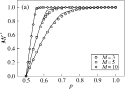
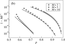
Figure 1: The comparison of numerical results for the optimal investment fraction $f^{*}$ (obtained using Mathematica, shown as symbols) with the analytical results given in Eq. (10) and Eq. (11) (shown as solid lines). (a) The total investment $Mf^{*}$ as a function of $p$. (b) To judge better the approximation for a saturated portfolio, the univested fraction $1-Mf^{*}$ is shown as a function of $p$.

4 Diversification vs information

In real life, investors have only limited information about the winning probabilities of the available risky games. These probabilities can be inferred using historical wins/losses data but these results are noisy and the analysis requires investor’s time and resources (the process of inference is investigated in detail in Sec. 5). At the same time, insider information can improve the investment performance substantially. A similar insider-outsider approach is discussed in the classical paper on efficient markets [14] and in a simple trading model [15]. We model the described situation by a competition of two investors who can invest in multiple risky games; each of the games has the winning probability alternating with even odds between $p+\Delta$ and $p-\Delta$ ($1/2<p\leq 1$, $0\leq\Delta\leq 1-p$). The insider focuses on one game in order to obtain better information about it—we assume that the exact winning probability is available to him. By contrast, the outsider invests in several games but knows only the time average $p$ of the winning probability. We shall investigate when the outsider performs better than the insider.

The insider knows the winning probability and thus can invest according to Eq. (5). If $p-\Delta>1/2$, he invests in each turn, if $p-\Delta\leq 1/2$, he invests only when the winning probability is $p+\Delta$. Combining the previous results, the exponential growth rate of the insider $G_{I}=\langle\ln W_{1}\rangle$ can be simplified to

$$G_{I}=\begin{cases}\frac{1}{2}[\ln 2+S(p+\Delta)]&p-\Delta\leq 1/2,\\ \frac{1}{2}[\ln 2+S(p+\Delta)]+\frac{1}{2}[\ln 2+S(p-\Delta)]&p-\Delta>1/2,\end{cases}$$ (12)

where $S(p)$ is the same as in Eq. (6). We assume that the outsider invests in $M$ identical and independent risky games. For him, each risky game is described by the average winning probability $p$. Consequently, the exponential growth rate of his investment is given by Eq. (8) and for the optimal investment fractions results from the previous section apply.

The limiting value of $\Delta$, above which the insider performs better that the outsider, is given by

$$G_{I}(p,\Delta)=G_{O}(p,M).$$ (13)

Due to the form of $G_{I}(p,\Delta)$, it is impossible to find an analytical expression for $\Delta$. An approximate solution can be obtained by expanding $G_{I}(p,\Delta)$ in powers of $\Delta$; first terms of this expansion have the form

$$G_{I}(p,\Delta)=\begin{cases}\tfrac{1}{2}\,\Big{[}G_{\mathrm{K}}(p)+\Delta\big{(}\ln p-\ln[1-p]\big{)}+\frac{\Delta^{2}}{2}\Big{(}\frac{1}{p}+\frac{1}{1-p}\Big{)}\Big{]}&p-\Delta\leq 1/2,\\ G_{\mathrm{K}}(p)+\frac{\Delta^{2}}{2}\Big{(}\frac{1}{p}+\frac{1}{1-p}\Big{)}+\frac{\Delta^{4}}{12}\Big{(}\frac{1}{p^{3}}+\frac{1}{(1-p)^{3}}\Big{)}&p-\Delta>1/2.\\ \end{cases}$$

By substituting this to Eq. (13) we obtain a quadratic (when $p-\Delta\leq 1/2$) or biquadratic (when $p-\Delta>1/2$) equation for $\Delta$ which can be solved analytically. In this way we get $\Delta(p,M)$, for $\Delta<\Delta(p,M)$ the outsider performs better than the insider. When $p-1/2\ll 1$, the lowest order approximation is $\Delta(p,M)=(p-1/2)(\sqrt{2M}-1)$. To review the accuracy of our calculation, in Fig. 2 analytical results for $M=2,3,4$ are shown together with numerical solutions of Eq. (13) obtained using Mathematica. In line with expectations, the higher is the winning probability $p$, the harder it is for the insider to outperform the outsider.

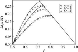
Figure 2: The limiting value $\Delta(p,M)$ when the investment performances of the insider investing in one game and the outsider investing in $M$ games are equal. Numerical solutions of Eq. (13) are shown as symbols, analytical results obtained as described in the text are shown as lines.

5 Finite memory problem

As already mentioned, in real life investors do not have information on the exact value of the winning probability $p$, it has to be inferred from the available past data. In addition, since $p$ can vary in time, it may be better to focus on a recent part of the data and obtain a fresh estimate. To model the described situation we assume that the investor uses outcomes from the last $L$ turns for the inference and that the winning probability $p$ is fixed during this period (a generalization to variable $p$ will be also discussed). The impact of uncertainty on the Kelly portfolio is investigated also in [16] where certain prior information and long-term stationarity of $p$ are assumed.

Let’s label the number of winning games in last $L$ turns as $w$ ($w=0,\dots,L$). The resulting knowledge about $p$ can be quantified by the Bayes theorem [17] as

$$\varrho(p|w,L)=\frac{\pi(p)P(w|p,L)}{\int_{0}^{1}\pi(p)P(w|L,p)\,\mathrm{d}p}.$$ (14)

Here $\pi(p)$ is the prior probability distribution of $p$ and $P(w|L,p)$ is the probability distribution of $w$ given the values $p$ and $L$. Due to mutual independence of consecutive outcomes, $P(w|L,p)$ is a binomial distribution and $P(w|L,p)=\binom{L}{w}p^{w}(1-p)^{L-w}$. We assume that all information available to the investor is represented by the observation of previous outcomes, no additional information enters the inference. The maximum prior ignorance is represented by $\pi(p)=1$ for $p\in[0,1]$ (a uniform prior). Consequently, Eq. (14) simplifies to

$$\varrho(p|w,L)=\frac{(L+1)!}{w!(L-w)!}\,p^{w}(1-p)^{L-w}.$$ (15)

This is the investor’s information about $p$ after observing $w$ wins in the last $L$ turns.

When in the Kelly game instead of the winning probability $p$, only the probability distribution $\varrho(p)$ is known, maximization of $G=\langle\ln W_{1}\rangle$ results in $f^{*}=2\langle p\rangle-1$. We prove this theorem for a special case of two possible winning probabilities $p_{1}$ and $p_{2}$, $P(p_{1})=P_{1}$, $P(p_{2})=P_{2}$, $P_{1}+P_{2}=1$ (extension to the general case is straightforward). The exponential growth rate can be now written as

$$G=(P_{1}p_{1}+P_{2}p_{2})\,\ln(1+f)+(1-P_{1}p_{1}-P_{2}p_{2})\,\ln(1-f).$$

This is maximized by $f^{*}=2(P_{1}p_{1}+P_{2}p_{2})-1$. Since $P_{1}p_{1}+P_{2}p_{2}=\langle p\rangle$, we have $f^{*}=2\langle p\rangle-1$. From Eq. (15) follows $\langle p\rangle=(w+1)/(L+2)$ and consequently

$$f^{*}(w,L)=\frac{2w-L}{L+2}$$ (16)

for $w\geq L/2$. Since we do not consider the possibility of short selling in this work, $f^{*}=0$ for $2w<L$. Even when $w=L$ (all observed game are winning), $f^{*}<1$. This is a consequence of the noisy information about $p$.

It is instructive to compute the exponential growth rate $G(p,L)$ of an investor with the memory length $L$. If $p$ is fixed during the game, we have

$$G(p,L)=\sum_{w=0}^{L}P(w|p,L)\,\big{[}p\ln(1+f^{*}(w,L))+(1-p)\ln(1-f^{*}(w,L))\big{]}.$$ (17)

The compounded return is consequently $\mathcal{R}(p,L)=\exp[G(p,L)]-1$. This result can be compared with $\mathcal{R}_{\mathrm{K}}(p)$ of an investor with the perfect knowledge of $p$ given by Eq. (7). In Fig. 3a, the ratio $\xi:=\mathcal{R}(p,L)/\mathcal{R}_{\mathrm{K}}(p)$ is shown as a function of $L$ for various $p$. As $L$ increases, the investor’s information about $p$ improves and $\xi\to 1$. Notice that when $p$ is smaller than a certain threshold (which we numerically found to be approximately $0.63$), $\mathcal{R}(p,L)<0$ for some $L$.

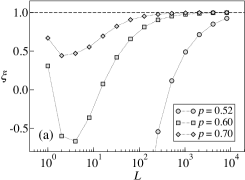
Figure 3: a) The ratio $\xi:=\mathcal{R}(p,L)/\mathcal{R}_{\mathrm{K}}(p)$ as a function of the memory length $L$. b) To check the accuracy of Eq. (19), the difference $d:=G_{\mathrm{K}}(p)-G(p,L)$ is shown as a function of $L$. Numerical results are shown as symbols, dotted lines are used to guide the eye. Eq. (19) suggests $d=1/(2L)$ which is shown as a solid line.

When $p$ is small, a very long memory is needed to make a profitable investment: e.g. for $p=0.51$, $L\geq 1\,761$ and for $p=0.52$, $L\geq 438$ is needed. This agrees with the experience of finance practitioners—according to them the Kelly portfolio is sensitive to a wrong examination of the investment profitability (for a scientific analysis of this problem see [18]). However, one should not forget about the prior distribution $\pi(p)$ which is an efficient tool to control the investment. For example, to avoid big losses in a weakly profitable game, $\pi(p)$ constrained to the range $[0,3/4]$ can be used. In turn, if the game happens to be highly profitable and $p>3/4$, such a choice of $\pi(p)$ reduces the profit.

Due to its complicated form, $G(p,L)$ given by Eq. (17) cannot be evaluated analytically. An approximate solution can be obtained by replacing summation by integration and noticing that for large values of $L$, $P(w;p,L)$ is approaches the normal distribution $g(w;\mu,\sigma)$ with the mean $\mu=Lp$ and the variance $\sigma^{2}=Lp(1-p)$. Then we have

$$G(p,L)\approx\int_{L/2}^{L}g(w;\mu,\sigma)h(w)\,\mathrm{d}w$$

where $h(w)=p\ln\big{[}(2w+2)/(L+2)\big{]}+(1-p)\ln\big{[}(2L+2-2w)/(L+2)\big{]}$. When $\sigma$ is small compared to the length of the range where $h(w)$ is positive, we can use the approximation

$$G(p,L)\approx h(\mu)+\frac{\sigma^{2}}{2}\left.\frac{\partial^{2}h}{\partial w^{2}}\right\rvert_{w=\mu}$$ (18)

which is based on expanding $h(w)$ in a Taylor series; a detailed discussion of this approximation can be found in [9]. It converges well when $h(w)$ is positive (and thus bounded) in the range where $g(w;\mu,\sigma)$ differs from zero substantially. Using $3\sigma$-range we obtain the condition $L\gtrsim 9p(1-p)/(p-1/2)^{2}$; when the equality holds, the final result obtained below has the relative error less than 10%. Using $h(w)$ written above, after neglecting terms of smaller order we obtain

$$G(p,L)\approx G_{\mathrm{K}}(p)-\frac{1}{2L}.$$ (19)

In Fig. 3, the quantity $d:=G_{\mathrm{K}}(p)-G(p,L)$ computed numerically is shown as a function of $L$ for various values of $p$, $d=1/(2L)$ following from Eq. (19) is shown as a solid line. It can be seen that in its range of applicability, the approximation works well. In addition, Eq. (19) yields a rough estimate of the minimum memory length needed to obtain $G(p,L)>0$ in the form $L_{\min}\approx 1/[2G_{\mathrm{K}}(p)]$.

When negative investment fractions are allowed, $f^{*}=(2w-L)/(L+2)$ also for $w<L/2$. As shown in Appendix, one can then obtain the series expansion of $G_{-}(p,L)$ (the subscript denotes that $f<0$ is allowed) in powers of $1/L$

$$G_{-}(p,L)=G_{\mathrm{K}}(p)-\frac{1}{2L}+\frac{11p(1-p)-1}{12p(1-p)L^{2}}-\frac{20p^{2}(1-p)^{2}-5p(1-p)-1}{12p^{2}(1-p)^{2}L^{3}}+\dots.$$ (20)

Notice that up to order $1/L$ it is identical with Eq. (19). When the terms shown above are used, Eq. (20) is highly accurate already for $L=20$. Despite it is based on a different assumption, it can be also used to approximate $G(p,L)$ discussed above; for small $L$ it gives better results than the rough approximation Eq. (19).

5.1 Another interpretation of the finite memory problem

The optimal investment of a gambler with the memory length $L$ can be inferred also by the direct maximization of the exponential growth rate. Then in addition to Eq. (17), from the investor’s point of view $G$ needs to be averaged over all possible values of $p$, leading to

$$G(L)=\int_{0}^{1}\pi(p)\,\mathrm{d}p\sum_{w=0}^{L}P(w;p,L)\,\big{(}p\ln[1+f(w,L)]+(1-p)\ln[1-f(w,L)]\big{)}.$$ (21)

This quantity can be maximized with respect to the investment fractions $f(w,L)$ which is equivalent to the set of equations $\partial G(L)/\partial f(w,L)=0$ ($w=0,\dots,L$). For $\pi(p)=1$ in the range $[0,1]$ this set can be solved analytically and yields the same optimal investment fractions as given in Eq. (16).

The statistical models described above use $\pi(p)$ as a model for the gambler’s prior knowledge of the winning probability $p$. This knowledge can be caused by the lack of gambler’s information but also it can stem from the fact that $p$ changes in time. Then $\pi(p)$ represents the probability that at a given turn, the winning probability is equal to $p$. Since such an evolution of game properties is likely to occur in real life, we investigate it in detail in the following paragraph. We remind that the possible changes of $p$ in time are the key reason why a gambler should use only a limited recent history of the game.

As explained above, the evolution of $p$ can be incorporated in $\pi(p)$. Consequently, if the changes of $p$ are slow enough to assume that within time window of the length $L$ the winning probability is approximately constant, the analytical results obtained in the previous section still hold and the optimal investment is given by Eq. (16). To test this conclusion, we maximized $G$ numerically with $f(w,L)$ as variables ($w=0,\dots,L$) for five separate realizations of the game, each with the length 1 000 000 turns and $L=10$. In each realization, the winning probability changed regularly and followed the succession $0.5\to 1\to 0\to 0.5$. As a maximization method we used simulated annealing [19, 20]. In Fig. 4, the result is shown together with $f^{*}(w,L)$ given by Eq. (16) and a good agreement can be seen. Thus we can conclude that with a proper choice of $\pi(p)$, the analyzed model describes also a risky game with a slowly changing winning probability.

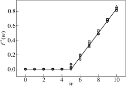
Figure 4: A comparison of the analytical fractions $f^{*}(w,L)$ with results numerical maximization of $G$ for $L=10$ and $N=1\,000\,000$. Various symbols are shown for five independent realizations of the game.

6 Conclusion

In this work we examined maximization of the exponential growth rate, originally proposed by Kelly, in various scenarios. Our main goal was to explore the effects of diversification and information on investment performance. To ease the computation, instead of working with real assets we investigated simple risky games with binary outcomes: win or loss. This allowed us to obtain analytical results in various model situations.

First, in the case when multiple independent investment opportunities are simultaneously available we proposed two complementary approximations which yield analytical results for the optimal investment fractions. Based on these results, we proposed a simple framework to investigate the competition of an uninformed investor (the outsider) who diversifies his portfolio and an informed investor (the insider) who focuses on one investment opportunity. We found the conditions when gains from the diversification exceed gains from the additional information and thus the outsider outperforms the insider.

Finally we investigated the performance of the Kelly strategy when the return distribution (in our case the winning probability of a risky game) is not known a priori. When the past game outcomes represent the only source of information, we found a simple analytical formula for the optimal investment. We showed that for a weakly profitable game, a very long history is needed to allow a profitable investment. As game properties may change in time and thus the estimates obtained using long histories may be biased, this is an important limitation. With short period estimates suffering from uncertainty and long period estimates suffering from non-stationarity, the Kelly strategy may be unable to yield a profitable investment.

Appendix A Developing a series expansion for $G_{-}(p,L)$

Since for the exponential growth rate $G_{-}(p,L)$ there is no closed analytical solution, we aim to obtain an approximate series expression. As in Sec. 5, $G_{-}(p,L)$ is given by the formula Eq. (17) with $f^{*}(w,L)=(2w-L)/(L+2)$ for $w=0,\dots,L$ and it can be rearranged to

$$G_{-}(p,L)=\ln\frac{2}{L+2}+\sum_{w=0}^{L}\frac{L!\,p^{w}(1-p)^{L-w}}{w!(L-w)!}\big{[}p\ln(w+1)+(1-p)\ln(L+1-w)\big{]},$$

To get rid of the logarithm terms we use $\ln z=-z\int_{0}^{\infty}(\gamma+\ln t)\mathrm{e}^{-tz}\mathrm{d}t$ where $\gamma\approx 0.577$ is the Euler’s constant. This formula follows directly from the usual integral representation of the Gamma function. Consequently, by the substitution $\tau:=\mathrm{e}^{-t}$ we obtain

$$\ln z=-z\int_{0}^{1}\big{[}\gamma+\ln(-\ln\tau)\big{]}\tau^{z-1}\mathrm{d}\tau.$$ (22)

After exchanging the order of the summation and the integration in $G_{-}(p,L)$ it is now possible to sum over $w$, leading to $G_{-}(p,L)=\ln\big{[}2/(L+2)\big{]}+R(p)+R(1-p)$ where

$$R(p) = \int_{0}^{1}\big{[}\gamma+\ln(-\ln\tau)\big{]}T(\tau,p,L)\,\mathrm{d}\tau,$$

$$T(\tau,p,L) = p(\tau p+1-p)^{L-1}\big{[}1-p+\tau p(1+L)\big{]}.$$

The substitution $\tau:=1-\varrho/L$ allows us to obtain series expansions of $T(\tau,p,L)$ and $\ln(-\ln\tau)$ in powers of $1/L$ which after integration lead to Eq. (20).

References

- [1] D. Duffie, Dynamic Asset Pricing Theory, 3rd Edition, Princeton University Press, 2001
- [2] E. J. Elton, M. J. Gruber, S. J. Brown, W. N. Goetzmann, Modern Portfolio Theory and Investment Analysis, 7th Edition, Wiley, 2006
- [3] J. L. Kelly, IEEE Transactions on Information Theory 2, 1956, 185–189
- [4] H. M. Markowitz, The Journal of Finance 31, 1976, 1273–1286
- [5] M. Finkelstein, R. Whitley, Advances in Applied Probability 13, 1981, 415–428
- [6] L. M. Rotando, E. O. Thorp, The American Mathematical Monthly 99, 1992, 922–931
- [7] S. Maslov, Y.-C. Zhang, International Journal of Theoretical and Applied Finance 1, 1998, 377–387
- [8] S. Browne, in Finding the Edge, Mathematical Analysis of Casino Games, eds. O. Vancura, J. Cornelius, and W. R. Eadington, University of Nevada, 2000
- [9] P. Laureti, M. Medo, Y.-C. Zhang, Analysis of Kelly-optimal portfolios, preprint, arXiv:0712.2771
- [10] L. Breiman, Fourth Berkeley Symp. Math. Stat. Prob. 1, 1961, 65–78
- [11] E. O. Thorp, in Finding the Edge, Mathematical Analysis of Casino Games, eds. O. Vancura, J. Cornelius, and W. R. Eadington, University of Nevada, 2000
- [12] T. M. Cover, Mathematical Finance 1, 1991, 1–29
- [13] C. Whitrow, Appl. Statist. 56, 2007, 607–623
- [14] S. J. Grossman, J. E. Stiglitz, The American Economic Review 70, 1980, 393–408
- [15] A. Capocci, Y.-C. Zhang, International Journal of Theoretical and Applied Finance 3, 2000, 511–522
- [16] S. Browne, W. Whitt, Adv. Appl. Prob. 28, 1996, 1145–1176
- [17] D. Sivia, J. Skilling, Data Analysis: A Bayesian Tutorial, Oxford University Press, 2006
- [18] F. Slanina, Physica A 269, 1999, 554–563
- [19] S. Kirkpatrick, C. D. Gelatt Jr., M. P. Vecchi, Science 220, 1983, 671–680
- [20] V. Černý, Journal of Optimization Theory and Applications 45, 1985, 41–51