Different fractal properties of positive and negative returns

Abstract

We perform an analysis of fractal properties of the positive and the negative changes of the German DAX30 index separately using Multifractal Detrended Fluctuation Analysis (MFDFA). By calculating the singularity spectra $f(\alpha)$ we show that returns of both signs reveal multiscaling. Curiously, these spectra display a significant difference in the scaling properties of returns with opposite sign. The negative price changes are ruled by stronger temporal correlations than the positive ones, what is manifested by larger values of the corresponding Hölder exponents. As regards the properties of dominant trends, a bear market is more persistent than the bull market irrespective of the sign of fluctuations.

89.20.-a,89.65.Gh

1 Introduction

Typical signals generated by economic systems are non-trivial structures which can be characterized in terms of the theory of multifractals. Interestingly, these structures are to some degree universal in real world, since they come not only from finance but also from diverse fields of science like physics [1, 2, 3, 4, 5], chemistry or biology [6, 7, 8, 9]. The concept of ”fractal world” was proposed by Mandelbrot in 1980s and was based on scale-invariant statistics with power law correlations [10]. In subsequent years this new theory was developed and finaly it brought a more general concept of multiscaling. It allows one to study the global and local behaviour of a singular measure, or, in other words, the mono- and multifractal properties of a system. In economy, mutifractality is a one of the well known stylized facts which characterize non-trivial properies of financial time series [11]. The stock price (or index) fluctuations can be described in terms of long-range temporal correlations by a spectrum of the Hölder-Hurst exponents and a set of fractal dimensions. Obtained results show that there exist n-point correlations in financial data, hardly detectable with commonly used methods like power spectrum or autocorrelation function. This discovery allows us to reject the efficient market hipothesis (EMH) with its main assumption that retuns are uncorrelated. Of course this kind of analysis is possible because appropriate methods were developed in last decade, among which the most popular are Wavelet Transform Modulus Maxima (WTMM) and Multifractal Detrended Fluctuation Analysis (MFDFA). As one of our recent works proved [16], the latter method is more reliable when the fractal properties of the analyzed signals are not known a priori and this is why we prefer to use this method here.

In a standard approach, one assumes that both the positive and the negative fluctuations have the same fractal or scaling properties; however, this may not apply to some particular cases [12]. For example, studying deeper characteristics of the financial signals we can infer that the nature of fluctuations can depend on their direction [13]. Therefore, in order to apprehend the studied processes completely we have to take into consideration also their sign. This is a reason why we decided to generalize MFDFA, to be able to analyze the positive and the negative changes separately.

This paper is organized as follows. In Section 2, we describe the data and explain the method in detail. Section 3 presents the results and disscusion and, finally, section 4 concludes.

2 Data and Methodology

All the calculations were performed for high-frequency data from the German stock market index DAX, comprising the two following periods: Period 1 from Nov 28, 1997 to Dec 30, 1999 and Period 2 from May 1, 2002 to May 1 2004. The time interval between consecutive records was $\Delta t=1$min. In each case the logarithmic returns were calculated: $g(i)=\ln(p(t_{i}+\Delta t))-\ln(p(t_{i}))$, where $p(t_{i})$ denotes an index value in a moment $t_{i}$. In addition, we removed all the overnight returns, because they cover a much longer time interval than 1 min and are also contaminated by some spurious artificial effects [14]. The length of the time series was approximately 268,000 points and it was enough to obtain statisticaly significant results. Moreover, we also analized two shorter time series (from Nov 28, 1997 to July 15, 1998 and from July 16 to Oct 15, 1998) which represent the periods of a bull and a bear market, respectively.

In order to investigate the fractal properties of the positive and the negative index fluctuations separetely, we modified the algorythm of MFDFA [15] such that the natural scale of signal and the length of possible temporal correlations is preserved. The main steps of this procedure can be briefly sketched as follows. At first one divides a given time series $g(i)$ into $M_{s}$ disjoint segments of length $s$ starting from the begining of the $g(i)$. To avoid neglecting the data which don’t fall into any segment (it refers to the data at the end of $g(i)$) the procedure is repeated starting this time from the end of the time series. Finally, one has $2M_{s}$ segments total. For each segment $\nu$, two signal profiles have to be calculated, separately for the positive (p) and the negative (n) fluctuations:

$$Y_{p}^{\nu}(i,s)=\Sigma_{k=1}^{i}g(Q^{\nu}(k))\quad i=1,...,N_{p}^{\nu}$$ (1)

$$Y_{n}^{\nu}(j,s)=\Sigma_{l=1}^{j}g(R^{\nu}(l))\quad j=1,...,N_{n}^{\nu},$$ (2)

where $Q^{\nu}(k)$ and $R^{\nu}(l)$ denote the sets of ($N^{\nu}_{p(n)}$) positions of the positive and the negative returns, respectively, within a segment $\nu$. In the next step we evaluate the variance for each segment:

$$F^{2}_{p}(\nu,s)=(\frac{1}{s}\Sigma_{k=1}^{N_{p}^{\nu}}\{Y_{p}^{\nu}(k,s)-P^{l}_{\nu}(k)\})$$ (3)

and

$$F^{2}_{n}(\nu,s)=(\frac{1}{s}\Sigma_{l=1}^{N_{n}^{\nu}}\{Y_{n}^{\nu}(l,s)-P^{l}_{\nu}(l)\}),$$ (4)

where $P^{l}_{\nu}()$ is a local trend in a segment $\nu$; it can be approximated by fitting an $l$th order polynomial $P^{l}_{\nu}$. This trend has to be substracted from the data. In this paper we use $l=2$ so we can eliminate l order possible trend in the profile and l-1 in the original time series. By averaging $F^{2}_{p}(\nu,s)$ and $F^{2}_{n}(\nu,s)$ over all $\nu$’s we obtain the $q$th-order fluctuation functions:

$$F_{p}^{q}(s)=\{\frac{1}{2M_{s}}\Sigma_{\nu-1}^{2M_{s}}[F^{2}_{p}(\nu,s)]^{q/2}\}^{1/q}$$ (5)

$$F_{n}^{q}(s)=\{\frac{1}{2M_{s}}\Sigma_{\nu-1}^{2M_{s}}[F^{2}_{n}(\nu,s)]^{q/2}\}^{1/q},$$ (6)

where $q\in\Re$ (in this paper, to make the results more readable, we use $-10<q<10$ [18]). Of course, this procedure has to be repeated for different segment lengths $s$. For a signal with fractal properies the fluctuation functions reveal power-law scaling

$$F_{p(n)}^{q}(s)\sim s^{h_{p(n)}(q)}$$ (7)

for large $s$. Family of the generalized Hurst exponents $h(q)$ characterizes complexity of an analyzed fractal. For a monofractal signal $h(q)=const$, while for multifractal signals $h(q)$ is a decreasing function of $q$. By knowing the spectrum of the generalized Hurst exponents for fluctuations with different signs we are able to calculate the singularity spectrum $f_{p(n)}(\alpha)$ according to the following relations:

$$\tau(q)=qh(q)-1$$ (8)

$$\alpha=\tau^{\prime}(q)\quad\textrm{and}\quad f(\alpha)=q\alpha-\tau(q),$$ (9)

where $\alpha$ is called the singularity exponent and $f(\alpha)$ is a fractal dimension of the set of all points $x_{0}$ such that $\alpha(x_{0})=\alpha$.

3 Results

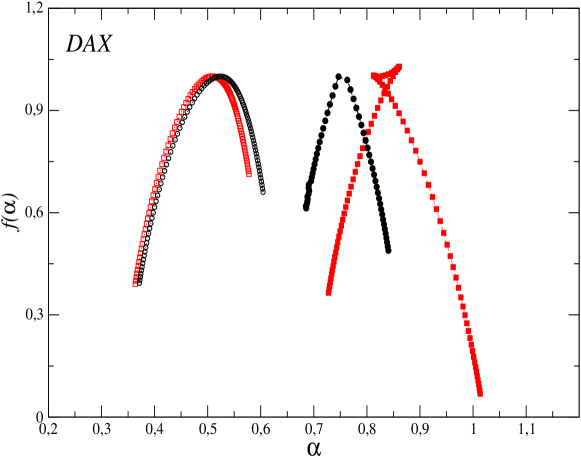
Figure 1: Singularity spectra for negative (red squares) and positive (black circles) DAX returns from Period 1 (Dec 1997 $-$ Dec 1999). Closed symbols refer to original and open to shuffled times series.

Figure 1 presents the $f_{p}(\alpha)$ and $f_{n}(\alpha)$ spectra for DAX in Period 1. It is easily visible that these spectra are different. For the negative fluctuations $f_{n}(\alpha)$ is rather wide ($\Delta\alpha\approx 0.3$) with its maximum placed at $\alpha^{max}_{n}\approx 0.85$. $f_{p}(\alpha)$ is much narrower ($\Delta\alpha\approx 0.15$) than in the former case; its maximum corresponds to $\alpha^{max}_{p}\approx 0.73$. In both cases, the positions of the maxima indicate a persistent character of the related index fluctuations. Naturally, if one looks at the scaling properties of volatility, one can expect such behaviour, but the shift between $f_{p}(\alpha)$ and $f_{n}(\alpha)$ as well as the difference in the spectra widths is a completely new observation. The $f_{n}(\alpha)$ is wider than its conterpart for the positive returns, suggesting that a richer multifractal (or more complex dynamics) is seen for the negative fluctuactions. For the shuffled signals, properties of the singularity spectrum do not depend on a direction of index changes. A lack of temporal correlations is manifested by a position of the spectrum at $\alpha^{max}_{p,n}\approx 0.5$. The difference between $f_{p}(\alpha)$ and $f_{n}(\alpha)$ in this case is rather meaningless and is a consequence of a finite sample size. Similar results we can see in Figure 2 (Period 2). Again, the $f_{n}(\alpha)$ is shifted to the right (maximum at $\alpha^{max}_{n}\approx 0.7$) relative to the spectrum for the positive returns ($\alpha^{max}_{p}\approx 0.65$); however, the difference is rather small in this case. Moreover, the multifractal spectrum for the negative index changes is substantially wider ($\Delta\alpha\approx 0.45$) than for $f_{p}(\alpha)$ ($\Delta\alpha\approx 0.25$) and this indicates a more complex dynamics governing behaviour of the negative returns. For the mixed-up data the spectra look almost identically with their maximum at $\alpha^{max}_{n,p}\approx 0.5$.

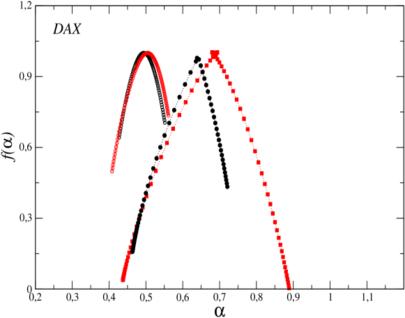
Figure 2: Singularity spectra for negative (red squares) and positive (black circles) DAX returns in Period 2 (May 2004 $-$ May 2006). Filled symbols refer to original and open to shuffled times series.

The multifractal characteristics of data can depend on a considered timeframe [17]. In particular, the multifractal spectrum can evolve in time to reflect the changing scaling properties of the data under study. In order to investigate how different market phases, associated with different behaviour of investors, can manifest themselves in the singularity spectra of the index returns, we applied our method to the bull and the bear phases, separately.

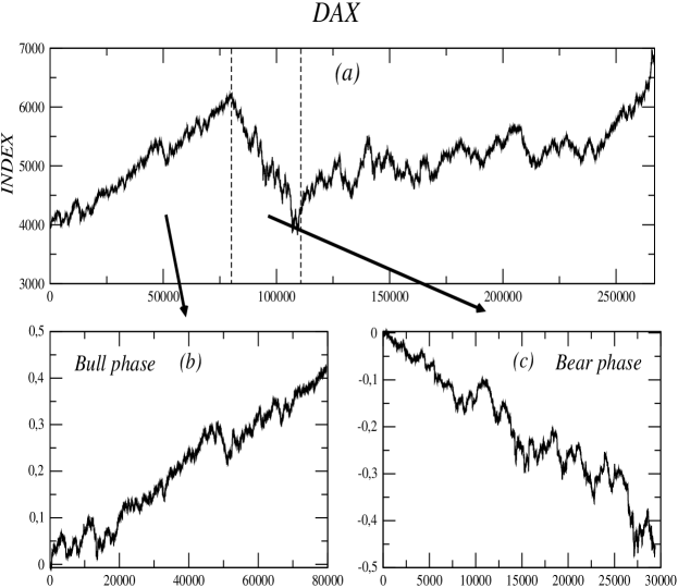
Figure 3: DAX daily closings in Period 1 (a) and the zoomed subperiods of index rise (b) and index decline (c).

Figure 3 shows the intervals of persistent growth and sudden decrease of the DAX index during Period 1. Results of our fractal analysis for these two intervals are presented in Figure 4. There is a clear difference between spectra for the growth and the decrease phase. For the period of slump the singularity spectra are shifted to the right, what means stronger correlations (both for the negative and the positive changes) than in case of boom. The position of maximum for the negative fluctuations is localized approximatetly at $\alpha^{max}_{n}\approx 0.87$ for the bear phase, whereas for the bull phase the maximum is placed at $\alpha^{max}_{p}\approx 0.82$; this gives the discrepancy $\Delta\alpha\approx 0.2$. For the positive fluctuations the difference is even more apparent and it totals $\Delta\alpha\approx 0.25$. By analyzing these relations between the spectra for the returns of different sign we can formulate a conclusion that the negative fluctuations are more persistent (or stronger correlated) than series of the opposite sign. This phanomenon is reflected in positions of the maxima of $f(\alpha)$ (higher $\alpha^{max}_{n}$).

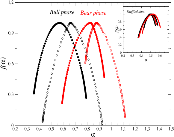
Figure 4: Comparison of $f(\alpha)$ spectra for phase of growth (black circles) and phase of decrease (red squares). Open symbols refer to negative and filled to positive DAX fluctuations.

The width of the singularity spectra for the bear phase is $\Delta\alpha\approx 0.35$ irrespective of a sign. For the bull phase, on the other hand, the $f(\alpha)$ spectrum is wider for the positive changes ($\Delta\alpha\approx 0.45$) than for the negative ones $\Delta\alpha\approx 0.35$; it shows richer multifractality in the former case. For the shuffed series the spectra have approximately the same width $\Delta\alpha\approx 0.2$ and are localized in a close vicinity of $\alpha\approx 0.5$. This demostrates that the temporal correlations present in time series are responsible for the discrepancy in fractal properties between the bull and bear phases.

4 Conclutions

We applied the MFDFA technique to show a difference in the fractal properties of the negative and the positive DAX index fluctuations. Our results suggest that a more persistent behaviour and often richer multifractality is associated with the negative price changes. This asymmetry disappears for the shuffled signals what implies that the temporal correlations are solely responsible for this effect. Moreover, our study of the index trends indicates a significant discrepancy between the bear and the bull market. Declining market is much more correlated than the rising one and can be described in terms of the Hölder exponent by $\alpha$ close to 1. We believe that the asymmetric fractal properties can give us an opportunity to better understand the mechanism that governs the stock market dynamics. From a practical point of view this fact can have applications in modeling and forecasting the stock market data and may be an important factor in risk evaluation.

References

- [1] C. Monthus, T. Garel, Phys. Rev. E 75, 051122 (2007).
- [2] B.M. Schäfer, W. Hofmann, H. Lampeitl, M. Hemberger, Nucl.Instrum.Meth. A 465, 394 (2001).
- [3] E. Nogueira Jr., R. F. S. Andrade, S. Coutinho, Physica A textbf360, 365 (2006).
- [4] A. Ordemann, M. Porto, H. E. Roman, S. Havlin, A. Bunde, Phys. Rev. E 61, 6858 (2000),
- [5] M. Barthelemy, S.V. Buldyrev, S. Havlin, H.E. Stanley, Phys. Rev. E (Rapid Comm.) 61, R3283 (2000).
- [6] C.-K. Peng, S. V. Buldyrev, S. Havlin, M. Simons, H. E. Stanley, and A. L. Goldberger, Phys. Rev E 49, 1685 (1994).
- [7] S. V. Buldyrev, A. L. Goldberger, S. Havlin, R. N. Mantegna, M. E. Matsa, C.-K. Peng, M. Simons, and H. E. Stanley, Phys. Rev. E 51, 5084 (1995).
- [8] A.Arneodo, Y. d’Aubenton-Carafa, E. Bacry, P.V. Graves, J.F. Muzy, C. Thermes, Physica D 96, 291 (1996).
- [9] J.M. Hausdorff,Y. Ashkenazy,C.-K. Peng, P.Ch. Ivanov, H.E. Stanley and A.L. Goldberger, Physica A 302, 138 (2001).
- [10] B.B. Mandelbrot, W.H. FreeMan, New York (1982).
- [11] Z. Eisler, J.Kertész, Physica A 343, 603 (2004).
- [12] K. Ohashi, L.A.N. Amaral, B.H. Natelson and Y. Yamamoto, Phys. Rev. E 68, 065204(R) (2003).
- [13] N.B. Ferreira, R. Menezes, D.A. Mendes, Physica A 382, 73 (2007).
- [14] A.Z. Górski, S. Drożdż, J. Speth, Physica A 316, 496 (2002) .
- [15] J.W. Kantelhardt, S.A. Zschiegner, E. Koscielny-Bunde, S. Havlin, A. Bunde, H.E. Stanley, Physica A 316, 87 (2002).
- [16] P. Oświȩcimka, J. Kwapień and Stanisaw Drożdż, Phys. Rev. E 74, 016103 (2006).
- [17] P. Oświȩcimka, J. Kwapień, S. Drożdż, A.Z. Górski, R. Rak, Acta Phys. Polon. B 37, 3083 (2006).
- [18] P. Oświȩcimka, J. Kwapień, S. Drożdż, Physica A 347, 626 (2005).