Abundance stratification in Type Ia Supernovae -
II: The rapidly declining, spectroscopically normal SN 2004eo

Abstract

The variation of properties of Type Ia supernovae, the thermonuclear explosions of Chandrasekhar-mass carbon-oxygen white dwarfs, is caused by different nucleosynthetic outcomes of these explosions, which can be traced from the distribution of abundances in the ejecta. The composition stratification of the spectroscopically normal but rapidly declining SN 2004eo is studied performing spectrum synthesis of a time-series of spectra obtained before and after maximum, and of one nebular spectrum obtained about eight months later. Early-time spectra indicate that the outer ejecta are dominated by oxygen and silicon, and contain other intermediate-mass elements (IME), implying that the outer part of the star was subject only to partial burning. In the inner part, nuclear statistical equilibrium (NSE) material dominates, but the production of ⁵⁶Ni was limited to $\sim 0.43\pm 0.05M_{\odot}$. An innermost zone containing $\sim 0.25M_{\odot}$ of stable Fe-group material is also present. The relatively small amount of NSE material synthesised by SN 2004eo explains both the dimness and the rapidly evolving light curve of this SN.

1 Introduction

Type Ia supernovae (SNe Ia), the thermonuclear explosions of carbon-oxygen white dwarfs that approach the Chandrasekhar mass limit (for a review, see Hillebrandt & Niemeyer 2000), are characterised by a simple optical light curve, showing a rise to maximum followed by a decline. The light curve is governed by the deposition of the $\gamma$-rays and the positrons produced by the decay of ⁵⁶Ni, which is copiously produced in the explosion and decays into ⁵⁶Co and hence ⁵⁶Fe (Arnett 1982; Kuchner et al. 1994), and by the diffusion in the expanding ejecta of the optical photons that are produced in the thermalisation process.

A correlation between the peak luminosity of SNe Ia and the shape of the light curve (Phillips 1993; Riess et al. 1996; Phillips et al. 1999), makes this class of SNe good standardizable candles. SNe Ia have been used to explore the expansion properties of the Universe out to about one third of its present age (Riess et al. 1998; Perlmutter et al. 1997).

While the SN luminosity is related fairly directly to the amount of ⁵⁶Ni ejected (Arnett 1982), so that the observed spread in peak luminosity suggests a corresponding spread in ⁵⁶Ni mass of about one order of magnitude ($\sim 0.1$ to $\sim 1M_{\odot}$) (Contardo, Leibundgut, & Vacca 2000; Stritzinger et al. 2006; Mazzali et al. 2007a), the light curve width depends primarily on the optical opacity in the ejecta, which is a function of both temperature and composition (Hoeflich et al. 1993). In the H-free ejecta of SNe Ia, line opacity dominates over continuum processes (Karp et al. 1977; Hoeflich et al. 1993; Pauldrach et al. 1996). Heavier elements have a thicker array of lines which, in combination with the rapid and differential expansion of the SN ejecta, causes the effective frequencies of the lines to overlap over the volume of the ejecta, efficiently blocking most UV and blue photons. For most of these photons the only way to escape is to be re-emitted in some less saturated transition in the red (Pinto & Eastman 2000; Mazzali 2000). This “fluorescence” process determines the shape of Type I SN spectra at early times, when the density is sufficiently large. Mazzali et al. (2001) showed that if the opacity is parametrised according to the average number of line transitions of the species that dominate the ejecta (singly and doubly ionised Si, S, Fe, Co and Ni for SNe Ia), SNe Ia that produce more ⁵⁶Ni are not only brighter but also have a larger opacity and hence broader light curves.

Additionally, different conditions within the white dwarf (e.g. metallicity) can lead to different nucleosynthesis of Fe-group isotopes (Timmes, Brown, & Truran 2003). For the same production of NSE material, SNe with a higher fraction of stable isotopes (e.g. ⁵⁴Fe, ⁵⁸Ni) over radioactive ⁵⁶Ni have light curves with a similar shape but different brightness. This may cause a spread in the observed luminosity-light curve shape relation (Mazzali & Podsiadlowski 2006).

Although an explanation for the observed behaviour of SNe Ia seems to have been found, a conclusive proof of the nature of the physical mechanism behind these explosions still eludes us. Subsonic deflagrations of Chandrasekhar-mass carbon-oxygen white dwarfs seem to be unable to produce the required energy and ⁵⁶Ni yield (Röpke et al. 2007). Detonations incinerate the white dwarf to NSE, and do not produce the IME that are observed in the spectra. A transition from a deflagration to a detonation (Khokhlov 1991) is a possible solution (Mazzali et al. 2007a), but its physical basis remains to be established, despite much effort (Röpke & Niemeyer 2007; Röpke 2007; Woosley 2007).

An alternative approach to the study of SNe Ia, rather than computing explosions and predicting their appearance, is to map the outcome of real events. This can be done performing spectrum synthesis of a time-series of SN spectra, following the progressive exposure of deeper and deeper layers of the ejecta as they expand.

Spectra at early times, in the so-called photospheric phase, probe only the outer half or so of the depth of the ejecta. A super-nebular phase then follows, during which the position of the pseudo-photosphere is extremely wavelength dependent and some features already follow nebular physics. A more direct and complete view of the inner ejecta can be obtained about one year after the explosion, when the gas in the young SN remnant is heated by collisions with the fast particles from the deposition of $\gamma$-rays and positrons and cools by emission of radiation, mostly in forbidden [Fe ii] and [Fe iii] lines. In this phase, the dominance of Fe lines testifies that ⁵⁶Ni is synthesised mostly in the deepest parts of the star, in line with theoretical expectations (e.g.  Iwamoto et al. 1999). A relation between the width of the Fe emission lines - which indicates the velocity of expansion of the bulk of ⁵⁶Ni - and both the SN peak brightness and the light curve decline rate (Mazzali et al. 1998) confirms that in more luminous SNe a larger fraction of the star is burned to NSE. It is therefore essential that SNe that have been monitored in the peak phase are also observed spectroscopically and photometrically in the nebular phase.

Only few examples of SNe Ia with very detailed time coverage were available (e.g.  Salvo et al. 2001) before the European Research and Training Network on the physics of Type Ia Supernovae (RTN) began collecting data of nearby SNe Ia systematically (e.g.  Benetti et al. 2004). Now, the availability of a sizable sample of SNe Ia with detailed observational coverage makes it possible to study in greater depth the properties of SNe of different luminosities. Since such differences are the result of different nucleosynthetic outcomes of the explosions, deriving the composition of the ejecta from the data should shed light on the details of the explosion process and it variations.

After initial efforts using homogeneous compositions (e.g.  Mazzali et al. 1993), the more computationally expensive analysis of a time series of spectra using stratified abundances has been attempted in only one case so far. Stehle et al. (2005, hereafter Paper I) mapped the ejecta of the normally luminous SN 2002bo from the centre out to $v\sim 20,000$  km s^-1. They showed that abundances are stratified but some mixing does occur. They detected burning products, namely stable Fe, Si and Ca, at very high velocities. This material gives rise to high velocity features (HVF), an apparently ubiquitous property of SNe Ia at the earliest phases (Mazzali et al. 2005). For SN 2002bo, the IME region extends down to $\sim 10,000$  km s^-1, below which NSE material dominates.

This distribution of elements in SN 2002bo seemed to favour a Delayed Detonation scenario. When the abundances derived in this sort of tomographic scan of the ejecta were used to generate opacities in a $\sim 10^{51}$ erg, Chandrasekhar-mass explosion with the density structure of the classic W7 model (Nomoto et al. 1984), the observed bolometric light curve was reproduced extremely well, including the early rise. This is induced by mixing out of ⁵⁶Ni, which is not predicted by most current explosion models but is indeed detected in early SN Ia spectra (Tanaka et al. 2008).

In this series of papers our aim is to describe the composition of the ejecta of SNe Ia with different luminosities and light curve decline rates. SN 2002bo was a SN Ia of average luminosity, which synthesised $\sim 0.5M_{\odot}$ of ⁵⁶Ni. In this second paper of the series, we address a SN at the dim end of the distribution of spectroscopically normal SNe Ia. SN 2004eo was observed by the RTN (Pastorello et al. 2007). It was a relatively underluminous event, with a $B$-band post-maximum decline rate $\Delta m_{15}(B)$$=1.46$ mag, which makes it very similar to the template SN 1992A. Like many such events, SN 2004eo showed a slow evolution of the Si ii line velocity (Benetti et al. 2005), measurements of which indicate that Si extended down to layers at $\sim 8500$  km s^-1, which is deeper than in SN 2002bo. The earliest spectra show a mild HVF in the Ca ii IR triplet, and possibly in Si ii 6355 Å.

The spectra and the light curve of SN 2004eo were presented by Pastorello et al. (2007). The sample, although temporally not as dense as for SN 2002bo, covers both the peak and the nebular phases, and is probably the best so far for a SN Ia of this luminosity group, offering a complete view of the ejecta of SN 2004eo except perhaps for the highest velocities.

In Section 2 our modelling is presented, and its limitations assessed. In Section 3 the modelling of the photospheric-epoch spectra is described, while the modelling of the nebular spectrum is discussed in Section 4. In Section 5 the abundance stratification obtained from the models is presented and discussed. In Section 6 we present and discuss a theoretical light curve computed on the basis of the abundances that have been derived. Finally, in Section 7 we give our conclusions.

2 Method

Our modelling strategy of is to follow the evolution of the SN in the early phases with a photosphere-plus-expanding-envelope code based on the Sobolev approximation, and to explore the innermost part of the ejecta modelling a single nebular spectrum taken $\sim 1$ yr later with a non-local thermodynamic equilibrium (non-LTE) nebular code.

For the early-time spectra, we used a Montecarlo code based on that first described by Mazzali & Lucy (1993) and updated by Lucy (1999) and Mazzali (2000). The code assumes a sharp photosphere, where the luminosity is emitted, and adopts the Sobolev approximation to follow energy packets in their propagation through the SN ejecta, which are represented by a density-velocity structure. The emerging luminosity $L$, the velocity of the pseudo-photosphere $v_{\rm ph}$, and an epoch $t$ since the explosion are required input, as is a set of depth-dependent abundances. Energy packets representing photon batches can interact with the ejecta via either line absorption or electron scattering. Upon absorption, a packet can be reprocessed into a different line, thus describing the process of line blocking which is essential for spectrum formation in Type I SNe (Mazzali 2000). No continuum processes are assumed to occur above the pseudo-photosphere. The properties of the radiation field and of the gas are iterated to convergence, temperature structure is established in radiative equilibrium and the ionization and excitation structures are computed using a modified nebular approximation that describes deviations from local thermodynamic equilibrium (for details, see Mazzali & Lucy 1993). We use the code version that employs abundance stratification, as discussed in Paper I.

The nebular spectrum has been modelled using a code that follows in 1D the propagation and the deposition of the $\gamma$-rays and positrons produced in the decay of ⁵⁶Ni into ⁵⁶Co and hence ⁵⁶Fe using a Montecarlo scheme (Cappellaro et al. 1997). Gas heating by the fast particles created upon $\gamma$-ray and positron deposition and the consequent cooling via line emission are described in non-LTE (Axelrod 1980; Ruiz-Lapuente & Lucy 1992; Mazzali et al. 2001). Stratification in density and abundance is used, as in Mazzali et al. (2007b).

Before we describe our results in detail, it is necessary to discuss the possible limitations of this method. Extracting the element distribution from a series of SN spectra is an ill-posed inverse problem: too many of the parameters that are used to compute the synthetic spectra are not known. In particular, assuming a certain density distribution artificially narrows down the number of possible solutions. Here we adopt the density-velocity distribution of W7 (Nomoto et al. 1984), for both the early and late-time modelling. Although W7 describes a more luminous SN Ia than SN 2004eo, it represents a typical density structure. Possible uncertainties related to using that particular model are discussed in Section 7. On the other hand, using any other explosion model is no better method, as the uncertainties related to the particular model would simply compound with those related to the spectrum synthesis codes.

Additional caveats stem from the design of the code that we use to model the photospheric-phase spectra. The use of a sharp photosphere is very effective, and it keeps the analysis free from the details of the explosion model, but it does not correspond to reality, in particular at times after maximum, when the photosphere resides within the ⁵⁶Ni zone and consequently a significant fraction of the $\gamma$-ray deposition occurs above the photosphere. These photons may alter both the flux level and the line profiles. Fortunately, this is mitigated by the decreasing density, which guarantees that even at advanced stages most deposition still occurs below the photosphere.

Additionally, since the nebular spectra do not suffer from this problem, and since the velocities sampled by the nebular lines exceed 7000 km s^-1, combining early photospheric-epoch results for the outer ejecta and late nebular ones for the inner ejecta we effectively avoid being too affected by the lesser accuracy of the post-maximum models.

Another shortcoming is the fact that we use a one-dimensional approach, while in reality SNe Ia ejecta may be affected to some extent by aspherical effects. However, three-dimensional spectral modelling can only be attempted starting from an explosion model, or the number of free parameters would be impossibly large, and it is a path that runs contrary to our approach.

When modelling spectra, it is practically impossible to establish objective criteria with which to judge the goodness of a fit. In fact, it is not fair simply to measure the deviation from the observed flux, because not all wavelengths have the same weight when it comes to deciding whether the physical quantitites that determine the spectrum are properly described. Deviations in wavelength are if possible of greater importance, because they signal an incorrect abundance, ionization or density distribution. Deviations in flux can be due to an incorrect luminosity or temperature, but also to incorrect line strengths, and these are again determined by density, ionization, and abundances. Therefore, a human observer is probably the best judge of the goodness of a fit.

In the case of a tomography experiment, it is not enough to fit a single spectrum, but the entire series must be reproduced by a single set of input data. There may be solutions that fit a single spectrum better than the one finally adopted, but the overall result may not be as good as that obtained with a different set. Therefore, a double compromise must be reached, on a set of input parameters that give both acceptable individual fits and on a fair reproduction of the spectral evolution.

Further details about the accuracy of our results are given in Sections 5 and 6.

3 Photospheric-epoch spectra

We have modelled 8 early-time spectra of SN 2004eo, covering epochs from $-11$ to $+22$ days relative to $B$ maximum. There are later spectra (see Pastorello et al. 2007), but we did not model them because the Montecarlo code becomes progressively less accurate at advanced epochs and because they probe very low velocities that are covered by the nebular spectrum.

We adopted a bolometric rise time of 19 days for SN 2004eo. This is somewhat less than the average $B$-band rise time (Riess et al. 1999), as motivated by the fact that dimmer SNe Ia seem to rise somewhat more rapidly than brighter ones. This is the consequence of the smaller opacity and the shorter photon diffusion time in the less nuclearly processed ejecta of dimmer SNe (Mazzali et al. 2001). The main input values for the synthetic spectra are recapped in Table 1, and the synthetic spectra are shown and compared to the observed ones in Figures 1 and 2. Using this approach, we map the abundance distribution in the ejecta. First we briefly discuss each spectrum in turn.

Table 1: Parameters of the synthetic spectra.

date	epoch	$\log L$	$v_{\rm ph}$	TB
	(days)	[erg s-1]	( km s-1)	(K)
19 Sept 2004	8.0	42.66	12000	13791
24 Sept 2004	12.7	43.03	10400	13926
27 Sept 2004	16.4	43.07	9500	12424
2 Oct 2004	21.4	43.10	9000	10621
7 Oct 2004	26.4	43.00	7300	10060
11 Oct 2004	30.4	42.85	6000	9499
14 Oct 2004	33.4	42.74	4700	9746
21 Oct 2004	40.4	42.53	2800	10367

3.1 19 September 2004: $-11$ days

The earliest spectrum of SN 2004eo has an epoch of $\sim 8$ days after explosion (Figure 1a). Although the SN was not a very luminous one, at this early epoch the small size of the ejecta results in a relatively high temperature, as shown by the fact that the two Fe features in the blue, near 4300 and 4800 Å, are dominated by Fe iii lines. Other strong features are due to Ca ii, Si ii, S ii, O i. The ratio of the two Si ii lines ($\lambda 5972$ and 6355 Å), which is a good temperature indicator (Nugent et al. 1995) is rather large. As shown by Hachinger et al. (2008), this is not directly the effect of a low temperature, as then the ratio would show the opposite trend, nor is it caused by Ti ii lines, as claimed by Garnavich et al. (2004), as in that case the much stronger Ti ii lines in the blue would completely change the spectrum. It is the result of saturation of the 6355 Å line as Si ii becomes more abundant with respect to Si iii going to lower luminosities, hence lower temperatures. So this is only indirectly the effect of temperature. In the UV, the spectrum is blocked by Fe ii, Fe iii, Ni ii, Ti ii, Ti iii, Cr ii, Cr ii and Mg ii lines. The flux redistribution caused by line blocking determines the properties of the optical spectrum.

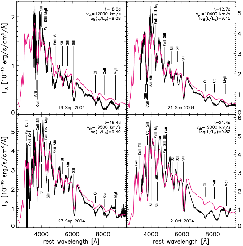
Figure 1: Fits to the earliest 4 spectra of SN 2004eo. Basic input parameters are shown and line identifications are marked. The spectra are as follows: a) (top left): $t=-11$ days; b) (top right): $t=-6$ days; c) (bottom left): $t=-3$ days; d) (bottom right): $t=+2$ days.

3.2 24 September 2004: $-6$ days

The second spectrum has an epoch of 12.7 days after explosion (Figure 1b). The increase in luminosity does not keep up with the increase in size, and the temperature is slightly lower. Most lines and their strength ratios are however similar to the previous epoch, since the temperature drop is small. The most noticeable change is the increased strength of the S ii complex near 5500 Å ($\lambda\lambda 5433,5454$ Å for the bluer feature, $\lambda\lambda 5606,5640$ Å for the redder one). This is indicative both of recombination and of an increased sulphur abundance as deeper layers are exposed. The abundance of silicon is also higher near the photosphere, but this has less of an effect on the Si ii lines, which were already quite strong in the earlier spectrum. In both this and the previous spectrum, the strength of the O i 7774 Å line indicates that a significant fraction of the outer layers was left unburned or only partially burned, as indicated by the absence of carbon lines (Mazzali 2001).

3.3 27 September 2004: $-3$ days

In the third spectrum, the last before $B$ maximum with an epoch of 16.4 days after explosion, the trend towards lower temperatures continues, while again the most apparent evolution is in the strength of the S ii lines (Figure 1c). The IME abundances are not much higher at this depth (9500  km s^-1), and reach a maximum here. The features that characterise the spectrum are the same as at the previous epoch. In all the pre-maximum spectra the near-IR continuum is reproduced reasonably well by the model, which never overestimates the flux by more than 20%. This indicates that the opacity, which is mostly due to lines, is sufficiently large at optical wavelengths that the assumption of an underlying black body is not grossly incorrect. Line blocking in the UV is stronger in this spectrum, as the photosphere moves inwards and more metals can absorb UV photons.

3.4 2 October 2004: $+2$ days

The spectra soon after maximum show subtle but significant differences with respect to the pre-maximum ones. In particular, starting with the spectrum of 2 October 2004, which has an an epoch of 21.4 days after explosion (Figure 1d), Fe ii  dominates over Fe iii. This is clearly seen in the shape of the feature near 4800 Å, which now shows strong Fe ii multiplet 48 lines (4923, 5018, 5169 Å) and has the characteristic shape of spectroscopically normal but relatively dim SNe Ia. Also, the O i 7774 Å line became weaker, indicating that the oxygen content near this rather deep (9000  km s^-1) photosphere is small or zero. The ionization of other ions that determine the UV also changes, as it does for iron, so that now Ca ii, Ti ii and Cr ii, together with Fe ii, determine the UV opacity. On the other hand, this spectrum still has a rather blue optical pseudo-continuum.

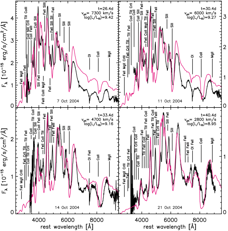
Figure 2: Fits to the spectra of SN 2004eo in the post-maximum phase. Basic input parameters are shown and and line identifications are marked. The spectra are as follows: a) (top left): $t=+7$ days; b) (top right): $t=+11$ days; c) (bottom left): $t=+14$ days; d) (bottom right): $t=+21$ days.

The model reproduces the observed spectrum at least bluewards of $\sim 6500$ Å, with a near-photospheric composition that is still dominated by IME, but where ⁵⁶Ni is increasing. The mass enclosed below the photosphere is now $\sim 0.8M_{\odot}$, and we are beginning to see the bulk of the NSE material. The model now overestimates the continuum in the red, indicating that the assumption of an underlying black body is less appropriate at this epoch. The observed pseudo-continuum redwards of the Si ii 6355 Å line must be caused mostly by flux redistribution to the red from line processes that take place in the blue and UV. Thus, the luminosity used for the model is probably higher than the real value. Nevertheless, the strength of the synthetic O i 7774 Å line is comparable to that of the observed feature. This is important in order to estimate the oxygen abundance. In general the abundances are not very different from those of the last pre-maximum spectrum.

3.5 7 October 2004: $+7$ days

The next spectrum (Figure 2a) has an epoch of 26.4 days after explosion, and it continues to show the evolution towards lower temperatures (a larger ratio of the two Si ii lines, the growth of the Si ii-Fe ii feature near 4800 Å) that started from the earliest phases. The iron absorption is now much stronger, indicating that we are beginning to see the inner, fully burned zone. Placing the boundary of the transition between incomplete (IME-dominated) and complete (NSE-dominated) burning zones somewhere between 7000 and 9000  km s^-1 one derives, using W7, an upper limit to the NSE mass of $\sim 0.7M_{\odot}$. This is in agreement with the results of Mazzali et al. (2007a).

3.6 11 October 2004: $+11$ days

In this spectrum (Figure 2b), at an epoch of 30.4 days after explosion, the low temperature begins to affect the pseudo-continuum significantly: the shape of the spectrum is now much redder. Fe ii lines have grown in strength. Not only is the Ni abundance higher, but ⁵⁶Co is decaying to ⁵⁶Fe. The fraction of stable Fe is also larger. This is a feature of SN 2004eo which is also borne out by the analysis of the nebular spectra (see Sect. 3). At this and later epochs, the feature near 5900 Å is probably contaminated by Na i D.

3.7 14 October 2004: $+14$ days

This spectrum (Figure 2c) has a nominal epoch of 33.4 days after explosion, and is very similar to the one obtained three days earlier. Most features are the same as in the previous epoch. The Na i D line is growing in strength, as is typical especially of dim SNe Ia. This feature is not reproduced because of the well-known uncertainty in the sodium ionization (e.g.  Mazzali et al. 1997). Although the photosphere is now very deep (4700  km s^-1), the Ca ii IR triplet absorption seems to reach even lower velocities, possibly suggesting the need for a higher calcium abundance at low velocity, or an incorrect estimate of the ionization there. The composition is dominated by ⁵⁶Ni (60% by mass) and stable Fe (35% by mass), the rest being mostly silicon and sulphur. This agrees with the nebular spectrum, which samples the region of the ejecta that is near the photosphere at this epoch.

3.8 21 October 2004: $+21$ days

The last of the early-time spectra we modelled has an epoch of 40.4 days after explosion (Figure 2d). It is very red, and it shows deep and broad absorptions. The strong emissions are still P-Cygni components caused by the absorption blends: the epoch is still too early for nebular emission lines to emerge, as indicated by the good fit to the Ca ii IR emission component. The broad features near 4500 and 5000 Å are caused by Fe ii lines, although some Ti ii contributes to the bluer feature, as it does in very underluminous SNe (Filippenko et al. 1992). The Na i D line is becoming very strong, while other lines are the same as at earlier epochs.

The synthetic spectrum matches the observed one surprisingly well, considering the advanced epoch and the very deep photosphere (2800  km s^-1), which suggests that the assumption of a grey photosphere is not unreasonable at this epoch. The reason for this is probably the fact that since iron dominates the composition near the photosphere, Fe ii, Ti ii, and, further to the red, Co ii lines effectively block the radiation and form a pseudo-continuum throughout the optical domain. The composition obtained agrees with that derived from the late-time spectrum (Sect. 3).

4 The nebular epoch

One nebular-epoch spectrum of SN 2004eo was presented in Pastorello et al. (2007). It was obtained 227 days after $B$ maximum, on 16 May 2006. We use this spectrum to investigate the structure and composition of the inner ejecta. The modelling results were already included in the compilation of Mazzali et al. (2007a), but the spectrum has been recalibrated because of scatter in the photometry and the values are therefore slightly different.

A one-zone version of the nebular code can be used to determine basic parameters as in Mazzali et al. (1998). The intrinsic width of the emission lines required to match the broad blends is 7300  km s^-1, which is on the low side of the distribution of line widths in SNe Ia (Mazzali et al. 1998). Nevertheless there is good overlap in velocity space between the most advanced photospheric epoch spectra that we modelled and the nebular spectrum, ensuring complete coverage of the ejecta and the consistency of the analysis. Material at velocities above 8000  km s^-1makes a negligible contribution to the nebular spectrum, indicating that the densities are too low and that ⁵⁶Ni is not present in any large amount at those velocities.

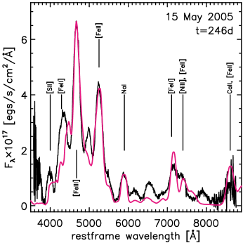
Figure 3: The nebular-epoch spectrum of SN 2004eo and a synthtic match.

For the stratified modelling the density stratification of W7 is again adopted, and the depth-dependent abundances are modified in order to fit the spectrum.

The abundances in the nebula are dominated by NSE material. The best fit (Figure 3) includes a ⁵⁶Ni mass of $0.38M_{\odot}$, located mostly between velocities of 2000 and 8000  km s^-1. The abundance of ⁵⁶Ni reaches $\sim 0.65$ by mass between 3000 and 7000  km s^-1. The innermost zone is dominated by stable Fe and Ni. This is necessary in order to avoid the formation of sharp emission peaks for the strongest [Fe iii] and [Fe ii] lines and to achieve an ionization balance that gives the correct ratio of the [Fe iii]-dominated 4700 Å line and the [Fe ii]-dominated 5200 Å line. The mass of stable Fe is $0.27M_{\odot}$, so that the total NSE mass is $0.65M_{\odot}$ (the mass of stable Ni is very small, in order to avoid a strong [Ni ii] emission near 7000 Å.

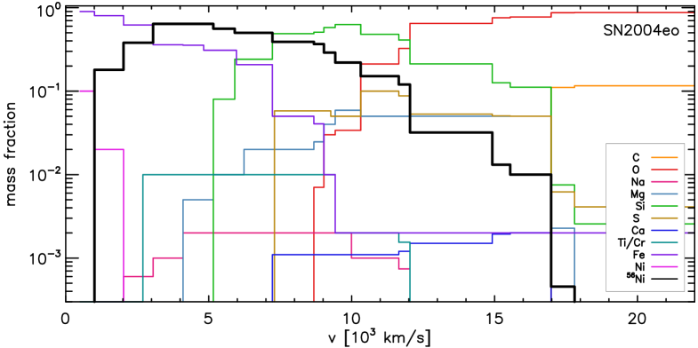
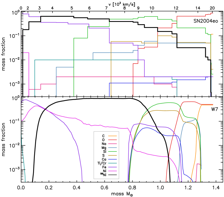
Figure 4: Distribution of the principal elements in the ejecta of SN 2004eo as derived from the spectral fitting. a) [top]: distribution in velocity space. b) [middle]: distribution in mass coordinates. c) [bottom]: distribution in mass coordinates of the W7 model (Nomoto et al. 1984).

The strongest observed emissions are fitted quite accurately. Many of the weaker lines that are not reproduced are weak Fe or Co lines, for which the collision strengths are not well known. The poor reproduction of those features means that we may be underestimating the ⁵⁶Ni mass by $\sim 5$%. Apart from the strong [Fe ii] and [Fe iii] lines, Na i D is clearly visible, as are Ca ii lines, which are however strongly affected by [Fe ii] emission. Mg i] 4700 Å contributes to the blue wing of the 4700 Å feature: a Mg mass of $0.04M_{\odot}$ is obtained from the fit. Silicon does not have strong lines in the optical domain, but it has a cooling effect since it produces lines in the IR, notably at 1.6 microns. A low upper limit for the sulphur abundance can be established from the line near 4000 Å. The oxygen abundance must be very low at velocities below 8000 km s^-1, or a strong [O i] 6300 Å line would form. The carbon abundance must also be very low, or [C i] emission would affect the blue part of the Ca ii IR triplet emission. The abundances above 8000  km s^-1are the same as those derived from the early-time modelling. Between 2800 and 7000  km s^-1some difference exists, but this is never more than 10%.

5 Abundance stratification

Connecting the results of early and late-time spectral modelling, we can reconstruct the abundance distribution as a function of depth in the ejecta. The results are shown in Figures 4a and 4b. The 11 most abundant species which contribute to the spectra are displayed. Minor species cannot be treated accurately owing to the lack of significant spectral features. Figures 4a and 4b show that oxygen dominates the outer ejecta, down to $\sim 12000$ km s^-1. This is not a particularly deep oxygen zone, despite the overall dimness of SN 2004eo, and it is comparable to most other SNe Ia (Mazzali et al. 2007a). The absence of carbon is noticeable: no carbon features are present that can be modelled, and the upper limit as constrained by the early spectra is very low (a few percent in the outer zones). This is also a feature of most SNe Ia, which may indicate partial burning of carbon to oxygen in the entire progenitor.

IME dominate at velocities between 7000 and 12000  km s^-1. Silicon is the most abundant IME, followed by sulphur and magnesium. The abundances of sodium and calcium are much smaller. IME are present out to the highest velocities surveyed by our spectral models, at a level of $\approx 10$% by mass. They do not extend significantly below $\sim 6000$  km s^-1, indicating again that the innermost part of the ejecta was completely burned to NSE. Among the NSE isotopes, ⁵⁶Ni is the most abundant species between 3000 and 7000  km s^-1, extending out to $\sim 12000$  km s^-1, while stable NSE isotopes (mostly stable Fe) dominate the inner 3000  km s^-1, as discussed in the previous section.

We can compare this distribution with those of W7 (Figure 4c) and of SN 2002bo (Paper I). In SN 2004eo NSE material does not extend as far out as in SN 2002bo, where the bulk reached $\sim 10,000$  km s^-1 but NSE material was present out to 15,000  km s^-1 at the 10% level, while W7 is somewhere in between and shows no mixing-out. The outer extent of the IME is similar in SNe 2004eo and 2002bo, confirming the result of Mazzali et al. (2007a). A peculiarity of SN 2004eo is the relatively large stable NSE material inner zone.

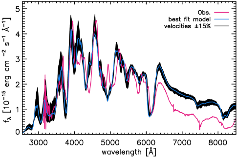
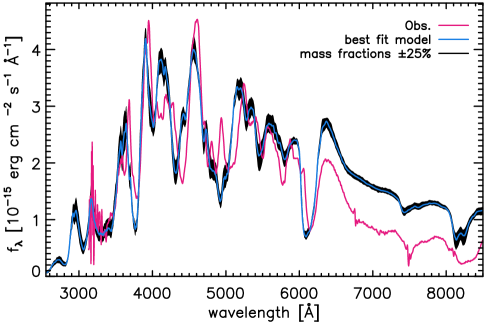
Figure 5: a) (top) Sensitivity of the results to velocity. The red line shows the observed $t=26.4$ day spectrum and the blue line is the best fit. The black band shows spectra computed changing the velocity boundaries of the various shells randomly by up to 15% with respect to the best-fit values. b) (bottom) Sensitivity to abundances within fixed velocity shells: same as above, but changing the abundances by up to 25% within each shell.

The abundance distribution we have presented is obtained from our best-fit models, as discussed in Section 2 above. It is instructive to verify the effect on the spectral fits of adopting different parameters. In Figures 5a and 5b we show the variation induced in the synthetic spectra by randomly varying the velocity boundaries of the various abundance shells by up to 15% (Fig. 5a) and the abundances by up to 25% (Fig. 5b). A relatively small change in the position of the shells can affect the result significantly. The sensitivity to abundance within a fixed shell is smaller, and the uncertainty can be estimated to be $\sim 25$% in the photospheric epoch. The examples shown here address the issue of fitting a particular spectrum. When trying to fit the entire time series, many of the solutions that may seem acceptable based on a single epoch do not result in a consistent fit of the spectral evolution. The masses of the NSE elements are estimated mostly from the nebular model, and have a smaller uncertainty.

6 A light curve model

In Paper I we could show that using the abundances derived from the spectral analysis to estimate the opacity in the ejecta a more accurate synthetic light curve could be obtained than any based on theoretical explosion models. In particular, the mixing out of ⁵⁶Ni is not predicted in most models, which therefore fail to reproduce the early rise of the light curve. Unfortunately, the situation is not quite as good for SN 2004eo, possibly because there are fewer very early spectra, which makes it difficult to constrain the abundances above 15000  km s^-1with high accuracy. In Figure 5 the bolometric light curve of SN 2004eo (Pastorello et al. 2007) is compared to a synthetic bolometric light curve obtained with a Montecarlo code based on that described in Cappellaro et al. (1997). In the calculation, the optical photons produced by the deposition of $\gamma$-rays and positrons diffuse in the ejecta, where they encounter an optical opacity which is determined by the abundance of the different isotopic species as follows:

$$\kappa_{opt}=0.1[M({\rm NSE})/M_{\odot}]+0.01[M({\rm IME})/M_{\odot}]$$ (1)

The synthetic light curve based on the abundance distribution derived from spectrum synthesis (Fig. 5, solid curve) resembles the observed one, with a peak at $\sim 19$ days, but it lies below the ”observed” one by $\sim 0.2$ mag at all epochs before $\sim 30$ days, although the tail is well reproduced.

The error introduced by the assumption of a sharp photosphere in the models for the photospheric-epoch spectra can be assessed by verifying in the synthetic light curve what fraction of the $\gamma$-ray deposition occurs above the momentary photosphere. For example, at maximum light less than 10% of the deposition occurs above the photosphere, which is then located at $\sim 9000$  km s^-1, above the bulk of ⁵⁶Ni. This fraction increases to $\sim 50$% by day 40, when the photosphere is well within the ⁵⁶Ni zone. However, the nebular spectrum covers velocities out to $\sim 9000$  km s^-1, and so the uncertainty caused by the use of a sharp photosphere is limited.

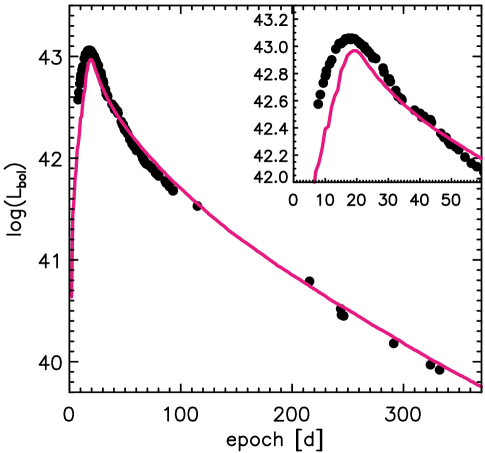
Figure 6: The bolometric light curve of SN 2004eo (Pastorello et al. 2007) compared to a synthetic light curve obtained using our Montecarlo light curve model (Cappellaro et al. 1997) and the abundances obtained from the spectral fitting discused in this paper. Although the synthetic light curve resembles the data, it fails to reach the same peak luminosity. The inset is an enlargement of the epoch of maximum.

One of the possible reasons for the discrepancy betwen the synthetic and observed light curves is the estimate of the mass and distribution of ⁵⁶Ni.

The synthetic light curve can be improved by changing the ⁵⁶Ni mass and distribution. Some possibilities are shown in Figure 6. First, if the amount of ⁵⁶Ni in the outer shells was underestimated because of poor spectral coverage or uncertainties in the spectral modelling at early times, a different rising part could be obtained. Adding ⁵⁶Ni at velocities above 10000  km s^-1 improves the rising part up to $\sim$ one week before maximum, but it still does not match the peak. In order further to improve the fit, it is necessary to play with the distribution of ⁵⁶Ni in a way that is not justified by the spectroscopic analysis. A model with enhanced ⁵⁶Ni in the region between 7000 and 10000  km s^-1 (Fig. 6, dashed line) results in a better fit of the peak. This model has $M({\rm{}^{56}Ni})=0.49M_{\odot}$, and $M({\rm NSE})=0.77M_{\odot}$. However, because of the very large ⁵⁶Ni mass this model is much too bright on the tail.

One further epicycle is then to remove ⁵⁶Ni at low velocities, below 6000 km s^-1. This model (Fig. 6, dotted line), with a total ⁵⁶Ni mass of $0.45M_{\odot}$ and $M(\rm{NSE})=0.76M_{\odot}$, fits the entire light curve, but is not physically justified. For example, a nebular spectrum based on this distribution of ⁵⁶Ni would not at all resemble the observations.

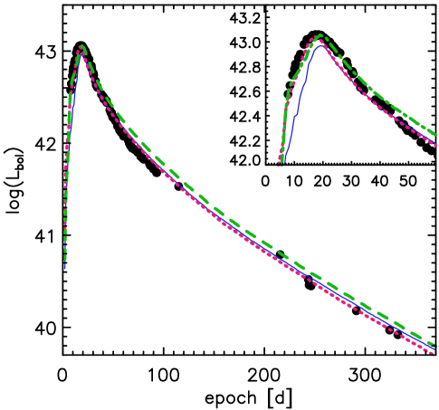
Figure 7: The bolometric light curve of SN 2004eo (Pastorello et al. 2007) compared to two synthetic light curves obtained by arbitrarily modifying the mass and distribution of ⁵⁶Ni. In the model shown as a dashed green line ⁵⁶Ni was added at velocities between 7000 and 10000  km s^-1, for a total M(⁵⁶Ni) $=0.49M_{\odot}$. This model fits the peak of the light curve, but is too bright on the tail. In the model shown as a dotted red line the additional ⁵⁶Ni at intermdiate velocities was compensated for by removing ⁵⁶Ni at velocities below 6000 km s^-1, for a total M(⁵⁶Ni) $=0.45M_{\odot}$. This model provides a good fit to the light curve but it is not physically motivated. The model from the abundance stratification [M(⁵⁶Ni) $=0.38M_{\odot}]$ is also shown for comparison (thin blue line).

The question is then what is the source of the discrepancy. There are at least 4 possibilities:

1) Calibration of the nebular spectrum. Incorrect calibration would result in an incorrect estimate of the ⁵⁶Ni content in the inner ejecta, and hence in an incorrect light curve. This is a possibility since there is scatter in the photometry obtained near the epoch of the nebular spectrum (Pastorello et al. 2007). It is however unlikely to result in a different relative distribution of ⁵⁶Ni and stable Fe-group isotopes, as this would directly affect the ionization balance and hence the line strength ratios.

2) Estimate of the amount of ⁵⁶Ni in the region between 7000 and 10000 km s^-1. The early-time spectra are relatively insensitive to variations of the ⁵⁶Ni mass in this velocity range: these layers are visible above the photosphere only after maximum, when most ⁵⁶Ni has decayed to ⁵⁶Co but only a small fraction of this has decayed to ⁵⁶Fe. Fe lines are therefore not greatly affected, and the effect of replacing nickel with cobalt is small. Nebular spectra, on the other hand, are also not very sensitive to small variations of the ⁵⁶Ni content at these velocities because of the low overall density.

3) Estimate of the bolometric correction and its evolution. Evidence for this may be the fact that even though the spectral fits at maximum require an input luminosity comparable to or somewhat lower than the corresponding $L_{Bol}$, the synthetic spectra thus obtained match the optical part of the observed spectra but are too bright in the near IR. Thus, the real value of $L_{Bol}$ at peak may actually be smaller than estimated in the bolometric light curve.

4) Uncertain treatment of the opacity. This is not likely to be a problem at late epochs, when the ejecta are transparent, but it may affect the light curve calculation near maximum. On the other hand, our synthetic light curve tracks the observed one quite well, the only problem being that it lies always below the data. This suggests that if there is a problem with the opacities, it lies in the $\gamma$-ray opacity, but this is a quantity that is well known and is unlikely to be grossly in error. The part of the light curve where the optical opacity is actually very likely to be incorrectly treated is between roughly 50 and 100 days, when the SN is making the transition to the nebular phase. This however has no effect on the estimate of the mass of ⁵⁶Ni either at the peak or on the tail of the light curve.

Alternatively, a direct estimate of the mass of ⁵⁶Ni may be attempted using the prescription of Stritzinger et al. (2006): $L=2\times 10^{43}M({\rm{}^{56}Ni})$. With a bolometric light curve peak of $1.15\times 10^{43}$ erg s^-1, this yields $M({\rm{}^{56}Ni})=0.57M_{\odot}$. This seems a very large value, given the results of the various light curve tests and the nebular spectrum. If we include ⁵⁶Ni in the inner part of the ejecta, as suggested by the spectroscopic modelling and by most explosion models, we can accommodate at most $0.49M_{\odot}$ of ⁵⁶Ni. This yields a good fit to the peak of the light curve, but it is too bright on the tail and it cannot reproduce the nebular spectra. Additionally, in all light curve models we have presented, we obtain a relation $L\sim 2.5\times 10^{43}M({\rm{}^{56}Ni})$, which again suggests that $M({\rm{}^{56}Ni})=0.45M_{\odot}$. The higher efficiency of conversion of $\gamma$-ray energy to optical light in our models with respect to the assumptions of Stritzinger et al. (2006) depends essentially on adopting a realistic density profile and a distribution of ⁵⁶Ni in the ejecta. Given all of the above uncertainties, a conservative estimate of the ⁵⁶Ni mass of SN 2004eo is $M({\rm{}^{56}Ni})=0.43\pm 0.05M_{\odot}$.

7 Conclusions

Despite the relatively small number of spectra available for modelling, a thorough description of the composition of the ejecta of SN 2004eo was obtained. This SN had a small ⁵⁶Ni mass for a normal SN Ia. The exact value is made somewhat uncertain by difficulties with deriving the bolometric light curve as well as by uncertainties in the calibration of the nebular spectrum and the behaviour of the optical opacity. Still our estimate, $M({\rm{}^{56}Ni})=0.43\pm 0.05M_{\odot}$, places SN 2004eo among the least luminous normal SNe Ia, along with the template SN 1992A.

A possible caveat concerns the total mass of the ejecta and the energy of the explosion. The assumption of the Chandrasekhar mass and of the W7 model yields a rather sensible abundance pattern and reasonably good synthetic spectra, suggesting that any deviation from that model should not be very large. Had the mass been significantly smaller, in our W7-based models we would have had to “hide” mass in elements that make a small contribution to the spectra: most likely oxygen in the photospheric phase and silicon in the nebular phase. This was however not required, and most elements included in the mixture do contribute significantly to the spectra at the appropriate epochs, via absorption lines at early times or emission lines in the nebular phase. As for the kinetic energy, applying the formula of Woosley et al. (2007), $E_{K}=[1.56M({\rm{}^{56}Ni})+1.74M({\rm stableNSE})+1.24M({\rm IME})-0.46]10^{51}$  erg, we obtain $E_{K}=1.1\pm 0.1\times 10^{51}$ erg. This is somewhat less than the original W7 energy ($1.3\times 10^{51}$ erg), but not so much less: the smaller contribution of burning to ⁵⁶Ni is in fact compensated by the larger production of IME, which contribute to the kinetic energy only $\sim 20$% less per unit mass synthesised, and by the large production of stable NSE isotopes, which actually contribute more to the kinetic energy than burning to ⁵⁶Ni. The main uncertainty regarding the kinetic energy comes from the outer extent of burning to NSE and the degree to which the outer carbon and oxygen were burned to IME. The zone between 9000 and 11000  km s^-1still contains some oxygen. A signature of the lack of incomplete burning products at high velocities may be seen in the lack of HVF’s, at least at the epochs sampled by our spectra.

In conclusion, within the uncertainties SN 2004eo was a Chandrasekhar-mass explosion of a CO white dwarf that produced a smaller amount of ⁵⁶Ni than average ($\sim 0.43M_{\odot}$). The amount of stable Fe-group material ($\sim 0.25M_{\odot}$), is somewhat larger than average (Mazzali et al. 2007a). The outer extent of IME ($\sim 1.1M_{\odot}$) is similar to most SNe Ia [the exception being those defined as High Velocity Gradient by Benetti et al. (2005)], so that the IME production was larger than average ($\sim 0.4M_{\odot}$). Since there is no indication of unburned carbon, most of the remaining $\sim 0.4M_{\odot}$ of material should be unburned oxygen.

Such a low luminosity explosion may be the result of a strong initial deflagration phase, during which NSE material is produced and the star pre-expands, so that if and when a delayed detonation occurs this is not very effective, burning material at low density mostly to IME only (Mazzali et al. 2007a). Uncertainties arise mostly from the spectral calibration, the bolometric correction and the lack of extremely early data, calling for more complete coverage of SNe Ia so that the parameters of the explosions can be derived with even greater precision. Nevertheless, SN 2004eo is an important piece in the description of the variety of SNe Ia and in the effort to understand their origin.

This research was supported by the European Union’s Human Potential Programme under contract HPRN-CT-2002-00303 “The Physics of Type Ia Supernovae” and by the National Science Foundation under Grant No. PHY05-51164. D.S. was supported by the Transregional Research Center TRR33 ”The Dark Universe” of the DFG.

References

- Arnett (1982) Arnett, D. 1982, ApJ, 253, 785
- Axelrod (1980) Axelrod, T. S. 1980, Ph.D. Thesis, Univ. of California, Santa Cruz
- Benetti et al. (2004) Benetti, S., et al. 2004, MNRAS, 348, 261
- Benetti et al. (2005) Benetti, S., et al. 2005, ApJ, 623, 1011
- Cappellaro et al. (1997) Cappellaro, E., Mazzali, P. A., Benetti, S., Danziger, I. J., Turatto, M., della Valle, M., & Patat, F. 1997, A&A, 328, 203
- Contardo, Leibundgut, & Vacca (2000) Contardo, G., Leibundgut, B., Vacca, W.D. 2000, A&A, 359, 876
- Filippenko et al. (1992) Filippenko, A. V., et al. 1992, AJ, 104, 1543
- Garnavich et al. (2004) Garnavich, P. M., et al. 2004, ApJ, 613, 1120
- Hachinger et al. (2008) Hachinger, S., et al. 2008, MNRAS, submitted
- Hillebrandt & Niemeyer (2000) Hillebrandt, W., & Niemeyer, J. C. 2000, ARA&A, 38, 191
- Hoeflich et al. (1993) Hoeflich, P., Mueller, E., & Khokhlov, A. 1993, A&A, 268, 570
- Karp et al. (1977) Karp, A. H., Lasher, G., Chan, K. L., & Salpeter, E. E. 1977, ApJ, 214, 161
- Khokhlov (1991) Khokhlov, A. M. 1991, A&A, 245, 114
- Kuchner et al. (1994) Kuchner, M. J., Kirshner, R. P., Pinto, P. A., & Leibundgut, B. 1994, ApJ, 426, L89
- Iwamoto et al. (1999) Iwamoto, K., Brachwitz, F., Nomoto, K., Kishimoto, N., Umeda, H., Hix, W. R., & Thielemann, F.-K. 1999, ApJS, 125, 439
- Lucy (1999) Lucy, L.B. 1999, A&A, 345, 211
- Mazzali (2000) Mazzali, P.A. 2000, A&A, 363, 705
- Mazzali (2001) Mazzali, P. A. 2001, MNRAS, 321, 341
- Mazzali et al. (1998) Mazzali, P.A., Cappellaro, E., Danziger, I.J., Turatto, M, Benetti, S. 1998, ApJ, 499, L49
- Mazzali et al. (1997) Mazzali, P. A., Chugai, N., Turatto, M., Lucy, L. B., Danziger, I. J., Cappellaro, E., della Valle, M., & Benetti, S. 1997, MNRAS, 284, 151
- Mazzali & Lucy (1993) Mazzali, P.A., Lucy, L.B. 1993, A&A, 279, 447
- Mazzali et al. (1993) Mazzali, P. A., Lucy, L. B., Danziger, I. J., Gouiffes, C., Cappellaro, E., & Turatto, M. 1993, A&A, 269, 423
- Mazzali et al. (2005) Mazzali, P. A., et al. 2005, ApJ, 623, L37
- Mazzali et al. (2001) Mazzali, P. A., Nomoto, K., Cappellaro, E., Nakamura, T., Umeda, H., Iwamoto, K. 2001, ApJ, 547, 988
- Mazzali & Podsiadlowski (2006) Mazzali, P. A., & Podsiadlowski, Ph. 2006, MNRAS, 369, L19
- Mazzali et al. (2007a) Mazzali, P. A., Röpke, F. K., Benetti, S., & Hillebrandt, W. 2007, Science, 315, 825
- Mazzali et al. (2007b) Mazzali, P. A., et al. 2007, ApJ, 670, 592
- Nomoto et al. (1984) Nomoto, K., Thielemann, F.-K., Yokoi, K. 1984, ApJ, 286, 644
- Nugent et al. (1995) Nugent, P., Phillips, M., Baron, E., Branch, D., Hauschild, P.H. 1995, ApJ, 455, L147
- Pastorello et al. (2007) Pastorello, A., et al. 2007, MNRAS, 377, 1531
- Pauldrach et al. (1996) Pauldrach, A.W.A., Duschinger, M., Mazzali, P.A., et al. 1996, A&A, 312, 525
- Perlmutter et al. (1997) Perlmutter, S., et al. 1997, ApJ, 483, 565
- Phillips (1993) Phillips, M.M. 1993, ApJ, 413, L105
- Phillips et al. (1999) Phillips, M.M., Lira, P., Suntzeff, N.B., Schommer, R.A., Hamuy, M., Maza, J. 1999, AJ, 118, 1766
- Pinto & Eastman (2000) Pinto, P.A., & Eastman, R.G. 2000, ApJ, 530, 757
- Riess et al. (1996) Riess, A. G., Press, W. H., & Kirshner, R. P. 1996, ApJ, 473, 88
- Riess et al. (1998) Riess, A. G., et al. 1998, AJ, 116, 1009
- Riess et al. (1999) Riess, A. G., et al. 1999, AJ, 118, 2675
- Röpke (2007) Röpke, F. K. 2007, ApJ, 668, 1103
- Röpke et al. (2007) Röpke, F. K., Hillebrandt, W., Schmidt, W., Niemeyer, J. C., Blinnikov, S. I., & Mazzali, P. A. 2007, ApJ, 668, 1132
- Röpke & Niemeyer (2007) Röpke, F. K. & Niemeyer, J. C. 2007, A&A, 464, 683
- Ruiz-Lapuente & Lucy (1992) Ruiz-Lapuente, P., & Lucy, L. B. 1992, ApJ, 400, 127
- Salvo et al. (2001) Salvo, M. E., Cappellaro, E., Mazzali, P. A., Benetti, S., Danziger, I. J., Patat, F., & Turatto, M. 2001, MNRAS, 321, 254
- Stehle et al. (2005) Stehle, M., Mazzali, P. A., Benetti, S., & Hillebrandt, W. 2005, MNRAS, 360, 1231 (Paper I)
- Stritzinger et al. (2006) Stritzinger, M., Leibundgut, B., Walch, S., & Contardo, G. 2006, A&A, 450, 241
- Tanaka et al. (2008) Tanaka, M., et al. 2008, ApJ, in press
- Timmes, Brown, & Truran (2003) Timmes, R., Brown, E.F., Truran, J.W. 2003, ApJ, 590, L83
- Woosley (2007) Woosley, S. E. 2007, ApJ, 668, 1109
- Woosley et al. (2007) Woosley, S. E., Kasen, D., Blinnikov, S., & Sorokina, E. 2007, ApJ, 662, 487