Decomposition of Complex Reaction Networks into Reactons

Abstract

The analysis of complex reaction networks is of great importance in several chemical and biochemical fields (interstellar chemistry, prebiotic chemistry, reaction mechanism, etc). In this article, we propose to simultaneously refine and extend for general chemical reaction systems the formalism initially introduced for the description of metabolic networks. The classical approaches through the computation of the right null space leads to the decomposition of the network into complex “cycles” of reactions concerned with all metabolites. We show how, departing from the left null space computation, the flux analysis can be decoupled into linear fluxes and single loops, allowing a more refine qualitative analysis as a function of the antagonisms and connections among these local fluxes. This analysis is made possible by the decomposition of the molecules into elementary subunits, called "reactons" and the consequent decomposition of the whole network into simple first order unary partial reactions related with simple transfers of reactons from one molecule to another. This article explains and justifies the algorithmic steps leading to the total decomposition of the reaction network into its constitutive elementary subpart.

Key words: metabolism; reacton; reaction network, stoichiometric matrix, left null space

Introduction

The dynamical analysis of complex reaction networks such as the ones characterizing interstellar chemistry (1), complex reaction mechanism (2) or metabolic functions (3) should be facilitated by algorithmic means to decouple these networks. It is conceivable that the presence of interesting dynamical phenomena like bifurcation or symmetry breaking is mainly due to structural antagonisms between reaction sub-networks provoking “threshold” effects. We propose in this article various algorithmic tools to allow such decoupling of complex reaction networks into simpler sub-networks. Any of these sub-networks will be restrictively concerned with the successive transformations of one given chemical group that will carry the name of “reacton” (in reminiscence of the organic chemistry “synthon”), defined as parts of the molecules that are never broken into smaller pieces by any reaction of the network (but internal rearrangements of the reactons are possible).

There has been a great amount of literature dedicated to the analysis of these reaction networks into sets of balanced reaction fluxes obtained by computing the right null space (or the “row” null space) of the stoichiometric matrix (4). However such analysis, while being performed on the complete molecules, leads to the discovery of fluxes that cross the whole set of reactions, making difficult the detection of antagonistic subsets and the automatic anticipation of interesting dynamical phenomena.

The computing of the left null space has been investigated by Famili and Palsson (5). They have shown that this leads to “pools of conserved metabolites” through the reaction network. Similar descriptions lead to concepts of “conservation analysis” (6) or “metabolic flux analysis” (7). Beyond what has been proposed in these previous studies, this leads to the total decomposition of each molecule into elementary subunits, the reactons. We argue later in the article that, such a conservation analysis allows to simplify the global reaction network into smaller sub-networks.

In order to simplify the reaction network analysis, the first step proposed in this article is to compute the left null space (or the “column” null space). The investigation of an optimal basis of this null space (this notion of "optimal basis" will be clarified later) reflects the existence of elementary reactons. Once the reactons are identified, the second step is to decouple the complete reaction network by simply restricting each sub-network to the single reacton that it is concerned with. Provided the reacton basis is correctly selected, it leads to substantially smaller networks.

Taking for instance the following reaction network:

$$X_{1}+X_{2} \xrightarrow{R_{1}} X_{3}$$ (1)

$$X_{3}+X_{4} \xrightarrow{R_{2}} X_{5}+X_{6}$$ (2)

$$X_{6} \xrightarrow{R_{3}} 2X_{2}.$$ (3)

the result of the algorithmic analysis performed on this system should automatically lead to the identification of an autocatalytic cycle based one the $X_{2}$, $X_{3}$ and $X_{6}$ compounds, as they are being recycled, of two incoming fluxes of $X_{1}$ and $X_{4}$, and two outgoing fluxes of $X_{5}$ and $X_{2}$, as represented in Figure 1. It is easy to detect the presence of two linear fluxes and one cycle, the most convenient building blocks to perform the following dynamical analysis (cycles and their intrinsic positive feedback are responsible for interesting dynamical effects) and to allow the anticipation of any interesting out-of-equilibrium phenomena such as the appearance of bifurcations.

1 Definition of the network

The studied chemical network is composed of $n$ different compounds noted $X_{i}$ for $1\leq i\leq n$, and $r$ different transformations noted $R_{j}$ for $1\leq j\leq r$. All these reactions are complete chemical transformations, and are thus mass balanced between reactant and products. In the example system of Eq. 1, we have $n=6$ and $r=3$.

Each reaction can be written in the form:

$$\forall j\in[1,r]\qquad R_{j}\quad:\quad\sum_{i=1}^{n}\nu_{i,j}X_{i}=0.$$ (4)

$\nu_{i,j}$ is the stoichiometric coefficient of the compound $i$ in the transformation $j$. It is by convention positive for products (formed compounds), and negative for reactants (disappearing compounds).

These stoichiometric coefficients can be gathered in a single $n\times r$ matrix $\overleftrightarrow{\nu}$. In this work, all matrices will be noted with a $\overleftrightarrow{\phantom{\nu}}$. The matrix for the system given in the example is the following $6\times 3$ matrix:

$$\overleftrightarrow{\nu}=\begin{pmatrix}-1&0&0\\ -1&0&+2\\ +1&-1&0\\ 0&-1&0\\ 0&+1&0\\ 0&+1&-1\\ \end{pmatrix}.$$ (5)

This stoichiometric matrix is actually formed by the juxtaposition of all reaction column vectors:

$$\overleftrightarrow{\nu}=\left(\overrightarrow{r}_{1}|\overrightarrow{r}_{2}|\cdots|\overrightarrow{r}_{r}\right).$$ (6)

All column vectors will be noted with a $\overrightarrow{\phantom{r}}$, to be distinguished from the row vectors noted with a $\overleftarrow{\phantom{c}}$. The purpose of this distinction is to easily know the dimension of the vectors, $\overrightarrow{a}$ being of dimension $n\times 1$, and $\overleftarrow{a}$ of dimension $1\times r$.

By noting $\overrightarrow{X}$ as the column vector of the $X_{i}$, Eq. 4 can be written as a matrix multiplication:

$$\overrightarrow{X}^{T}\overleftrightarrow{\nu}=\overleftarrow{0},$$ (7)

or, separating each reaction:

$$\forall j\in[1,r]\qquad\overrightarrow{X}^{T}\overrightarrow{r_{j}}=0.$$ (8)

The traditional analysis of the stoichiometric matrix relies on the calculation of its null spaces. The right null space, or the set of combinations of columns of the matrix that gives $\overrightarrow{0}$ can be expressed as (8):

$$\overleftarrow{\mathrm{Null}}(\overleftrightarrow{\nu}) = \left\{\overleftarrow{b}^{T}\quad|\quad\overleftrightarrow{\nu}\overleftarrow{b}^{T}=\overrightarrow{0}\right\}.$$ (9)

This corresponds to the set of cycles of reactions, i.e. the combinations of reactions that results in no global change inside the system (4). A base of this null space can be computed by the Gauss-Jordan elimination (9), and represented by:

$$\overleftarrow{\mathrm{Null}}(\overleftrightarrow{\nu})\quad:\quad\overleftrightarrow{\sigma}=\left(\begin{array}[]{c}\overleftarrow{\sigma_{1}}\\ \hline\cr\vdots\\ \hline\cr\overleftarrow{\sigma_{s}}\end{array}\right)\quad|\quad\overleftrightarrow{\nu}\overleftrightarrow{\sigma}^{T}=\overrightarrow{0}.$$ (10)

All the $\overleftarrow{\sigma_{k}}$ are linearly independent row vectors of the null space, each one being the row $k$ of the matrix $\overleftrightarrow{\sigma}$. The total matrix $\overleftrightarrow{\sigma}$ is thus full rank, and all vectors of the null space can be expressed as a linear combination of the $\overleftarrow{\sigma_{k}}$.

On the other hand, the left null space, i.e. the set of combinations of rows of the matrix that gives $\overleftarrow{0}$, can be expressed as (8):

$$\overrightarrow{\mathrm{Null}}(\overleftrightarrow{\nu}) = \overleftarrow{\mathrm{Null}}(\overleftrightarrow{\nu}^{T})$$ (11)

$$= \left\{\overrightarrow{a}\quad|\quad\overrightarrow{a}^{T}\overleftrightarrow{\nu}=\overleftarrow{0}\right\}.$$ (12)

This left null space of $\overleftrightarrow{\nu}$ is the right null space of $\overleftrightarrow{\nu}^{T}$. It corresponds to the mass balance in compounds (5). Similarly, a base of this null space can be represented as:

$$\overrightarrow{\mathrm{Null}}(\overleftrightarrow{\nu})\quad:\quad\overleftrightarrow{\sigma}=\left(\overrightarrow{\sigma_{1}}|\ldots|\overrightarrow{\sigma_{s}}\right)\quad|\quad\overleftrightarrow{\sigma}^{T}\overleftrightarrow{\nu}=\overleftarrow{0},$$ (13)

where $\overrightarrow{\sigma_{k}}$ indicates the column $k$ of the matrix $\overleftrightarrow{\sigma}$.

Molecule Decomposition into reactons

Elementary Reactons

A reacton is defined as a subpart of a molecule that is never broken into smaller parts by any of the reactions composing the network. The chemical reaction network can thus be seen as simple recombinations of reactons.

A first obvious category of reactons is composed of the atoms, but larger groups are more likely. Typically, in a polymerization system, monomers could be such reactons.

Molecules can be seen as linear combinations of reactons such as:

$$X_{i} = \sum_{k=1}^{a}\alpha_{i,k}A_{k}$$ (14)

$$\Leftrightarrow\quad\overrightarrow{X} = \overleftrightarrow{\alpha}\overrightarrow{A},$$ (15)

with $a$ being the total number of different reactons chosen for the decomposition. All the $\alpha_{i,k}$ are positive or zero integers, and represent the number of reacton $A_{k}$ in $X_{i}$. The decomposition of $X_{i}$ is represented by the vector $\overrightarrow{\alpha_{i}}$. The reactons can be represented as a column vector $\overrightarrow{A}$ of dimension $a$. The matrix $\overleftrightarrow{\alpha}$ of dimension $n\times a$ represents the decomposition of the whole set of molecules.

As molecules can always be at least decomposed into unbreakable atoms (no nuclear reaction is obviously considered here), there always exists at least one possible combination of reactons. Nevertheless, the computation of the left null space should provide us with more useful reactons in order to simplify the whole network into various subsets of "independent" reactive pathways.

Any reaction can be written in terms of reactons by substituting Eq. 14 in Eq. 4:

$$\sum_{i=1}^{n}\nu_{i,j}\sum_{k=1}^{a}\alpha_{i,k}A_{k} = 0$$ (16)

$$\sum_{k=1}^{a}\left(\sum_{i=1}^{n}\nu_{i,j}\alpha_{i,k}\right)A_{k} = 0$$ (17)

$$\Leftrightarrow\quad\overrightarrow{A}^{T}\overleftrightarrow{\alpha}^{T}\overleftrightarrow{\nu} = \overleftarrow{0}$$ (18)

There is a mass balance between each reacton $A_{k}$: they are never broken into smaller compounds, so that there is always the same number of every reacton for both reactants and products in any reaction. We thus have:

$$\forall j\in[1,r]~{},\forall k\in[1,a]\quad,\quad\sum_{i=1}^{n}\nu_{i,j}\alpha_{i,k} = 0$$ (19)

$$\Leftrightarrow\quad\forall k\in[1,a]\quad,\quad\overrightarrow{\alpha_{k}}^{T}\overleftrightarrow{\nu} = \overleftarrow{0}$$ (20)

Thus, we have according to Eq. 12 and Eq. 19:

$$\overrightarrow{\alpha_{k}} \in \overrightarrow{\mathrm{Null}}\left(\overleftrightarrow{\nu}\right)$$ (21)

All the vectors describing the decomposition of a molecule $X_{i}$ into reactons $A_{k}$, as it can be easily obtained by the atomic decomposition, are in the left null space of the stoichiometric matrix.

Let us take the system given in the example of Eq. 1-1, and further decompose it into small reactons (atoms):

$$\mathrm{CH_{4}O+CH_{2}O} \xrightarrow{R_{1}} \mathrm{C_{2}H_{6}O_{2}}$$ (22)

$$\mathrm{C_{2}H_{6}O_{2}+O_{2}} \xrightarrow{R_{2}} \mathrm{H_{2}O_{2}+C_{2}H_{4}O_{2}}$$ (23)

$$\mathrm{C_{2}H_{4}O_{2}} \xrightarrow{R_{3}} 2~{}\mathrm{CH_{2}O}.$$ (24)

This system is only for the sake of demonstration and has no real counterpart. A realistic system will be considered in the penultimate section. $X_{1}=\mathrm{CH_{4}O}$, $X_{2}=\mathrm{CH_{2}O}$, $X_{3}=\mathrm{C_{2}H_{6}O_{2}}$, $X_{4}=\mathrm{O_{2}}$, $X_{5}=\mathrm{H_{2}O_{2}}$, and $X_{6}=\mathrm{C_{2}H_{4}O_{2}}$. There are three atomic reactons: $A_{1}=\mathrm{C}$, $A_{2}=\mathrm{H}$ and $A_{3}=\mathrm{O}$. The mass balance in each of these reactons can be seen by the fact that all reactions are equilibrated. The matrix writing of this is:

$$\overleftrightarrow{\alpha}=[\overrightarrow{\alpha_{1}}|\overrightarrow{\alpha_{2}}|\overrightarrow{\alpha_{3}}]=\begin{pmatrix}1&4&1\\ 1&2&1\\ 2&6&2\\ 0&0&2\\ 0&2&2\\ 2&4&2\end{pmatrix}$$ (25)

It can be easily verified that the relation $\overleftrightarrow{\alpha}^{T}\overleftrightarrow{\nu}=\overleftarrow{0}$ is satisfied. This simple decomposition of the molecules of the reaction network into their atoms provides a first possible solution of the left null space.

Null Space Base and Optimal Reacton Decomposition

This a priori decomposition only gives a collection of reactons, that may not describe the whole null space. It is possible to compute a base of the left null space of $\overleftrightarrow{\nu}$ by a Gauss-Jordan elimination (9), represented by the matrix $\overleftrightarrow{\sigma}$:

$$\overrightarrow{\mathrm{Null}}\left(\overleftrightarrow{\nu}\right)\quad:\quad\overleftrightarrow{\sigma}=\left[\overrightarrow{\sigma_{1}}|\ldots|\overrightarrow{\sigma_{s}}\right]$$ (26)

all the $\overrightarrow{\sigma_{k}}$ vectors that are found respect Eq. 21 and thus result in one possible reacton decomposition. There is always a linear mapping from any set of reactons to the original set found by computing the null space. It is thus possible to derive any new and more convenient reacton decomposition from this preliminary set.

Of course, several basis are possible. It is therefore important to find an “optimal” decomposition. As the $\sigma_{i,k}$ represent the number of reactons present in each molecule, large values of $\sigma_{i,k}$ imply small reactons (because it means that more reactons are required to build the molecule). As a consequence, researching the linear combinations of the $\overrightarrow{\sigma_{k}}$ that compose the $\overrightarrow{\mathrm{Null}}\left(\overleftrightarrow{\nu}\right)$ while minimizing the individual $\sigma_{i,k}$ and maximizing the number of nought values will lead to a desired maximization of the size of the reactons. Obtaining a base of the null space composed of such larger reactons present great interest, as the larger molecular subparts that are never broken through the reactions are likely to represent fundamental building blocks of the system. This should lead to an optimal network decomposition characterized by a small number of reactons.

Computing the left null space base of the example system, by using the Gauss pivot method, gives the three following null vectors:

$$\overrightarrow{\mathrm{Null}}(\overleftrightarrow{\nu})\quad:\quad\begin{pmatrix}-1&+1&+1\\ 0&0&+1\\ -1&+1&+2\\ +1&0&0\\ 0&+1&0\\ 0&0&+2\end{pmatrix}$$ (27)

For a good representation of reactons, all the vector elements must be positive or zero integers. A new base can be searched for, by linearly combining the null vectors, aiming at maximizing the number of zero elements in each new vector.

The second and third reacton possess only positive values and thus can be kept as such. In order to eliminate the negative values of the first one, we can just add the two first reactons:

$$\overrightarrow{\mathrm{Null}}(\overleftrightarrow{\nu})\quad:\quad\overleftrightarrow{\sigma}=[\overrightarrow{\sigma_{1}}|\overrightarrow{\sigma_{2}}|\overrightarrow{\sigma_{3}}]=\begin{pmatrix}0&1&1\\ 0&0&1\\ 0&1&2\\ 1&0&0\\ 1&1&0\\ 0&0&2\end{pmatrix}$$ (28)

This decomposition can be seen as a better one than the atomic decomposition. The molecules are at most decomposed into $3$ reactons, instead of up to $10$. Moreover, two molecules ($X_{2}$ and $X_{4}$) are even composed of only one reacton, and can thus be identified as elementary building blocks of the system.

Elementary decomposition of reactons

Since we can express any reacton as a linear combination of the vectors of the null space base $\overleftrightarrow{\sigma}$, it is possible to link the elementary reactons to the atomic reactons. The elementary decomposition $\overleftrightarrow{\alpha}=\left(\overrightarrow{\alpha_{1}}|\ldots|\overrightarrow{\alpha_{a}}\right)$, for a system composed of $a$ atoms from $A_{1}$ to $A_{a}$, can be written as:

$$\overleftrightarrow{\alpha}\begin{pmatrix}A_{1}\\ \vdots\\ A_{a}\end{pmatrix}=\begin{pmatrix}X_{1}\\ \vdots\\ X_{n}\end{pmatrix}=\overrightarrow{X}.$$ (29)

The reacton decomposition $\overleftrightarrow{\sigma}$ composed of $s$ reactons from $S_{1}$ to $S_{s}$, can be written as:

$$\overleftrightarrow{\sigma}\begin{pmatrix}S_{1}\\ \vdots\\ S_{s}\end{pmatrix}=\overrightarrow{X}.$$ (30)

Expressing $\overleftrightarrow{\alpha}$ in terms of the null space base is equivalent to finding a matrix $\overleftrightarrow{T}$ so that:

$$\overleftrightarrow{\sigma}\overleftrightarrow{T}=\overleftrightarrow{\alpha}$$ (31)

Combining Eq. 29 and Eq. 30 gives:

$$\overleftrightarrow{\alpha}\overleftrightarrow{A} = \overleftrightarrow{\sigma}\overleftrightarrow{S}$$ (32)

$$\overleftrightarrow{\sigma}\overleftrightarrow{T}\overleftrightarrow{A} = \overleftrightarrow{\sigma}\overleftrightarrow{S}.$$ (33)

Because $\overleftrightarrow{\sigma}$ is full rank, it is possible to obtain the decomposition of the reactons into atom by:

$$\overleftrightarrow{S}=\overleftrightarrow{T}\overleftrightarrow{A}.$$ (34)

In the example of Eq. 22-24, linear combinations between $\overrightarrow{\alpha_{k}}$ and $\overrightarrow{\sigma_{k}}$ can easily be found:

$$\overrightarrow{\alpha_{1}} = \overrightarrow{\sigma_{3}}$$ (35)

$$\overrightarrow{\alpha_{2}} = 2\overrightarrow{\sigma_{2}}+2\overrightarrow{\sigma_{3}}$$ (36)

$$\overrightarrow{\alpha_{3}} = 2\overrightarrow{\sigma_{1}}+\overrightarrow{\sigma_{3}},$$ (37)

leading to:

$$\overleftrightarrow{\sigma}\begin{pmatrix}0&0&2\\ 0&2&0\\ 1&2&1\end{pmatrix} = \overleftrightarrow{\alpha}$$ (38)

$$\begin{pmatrix}S_{1}\\ S_{2}\\ S_{3}\end{pmatrix} = \begin{pmatrix}0&0&2\\ 0&2&0\\ 1&2&1\end{pmatrix}\begin{pmatrix}\mathrm{C}\\ \mathrm{H}\\ \mathrm{O}\end{pmatrix}.$$ (39)

As a consequence, this new decomposition, aiming for bigger reactons, gives the three following ones: $S_{1}=\mathrm{O_{2}}$, $S_{2}=\mathrm{H_{2}}$ and $S_{3}=\mathrm{CH_{2}O}$. We thus have $X_{1}=\mathrm{(H_{2})(CH_{2}O)}$, $X_{2}=\mathrm{(CH_{2}O)}$, $X_{3}=\mathrm{(H_{2})(CH_{2}O)_{2}}$, $X_{4}=\mathrm{(O_{2})}$, $X_{5}=\mathrm{(O_{2})(H_{2})}$, $X_{6}=\mathrm{(CH_{2}O)_{2}}$. It can be checked that all the reactions of the example can be written as association and dissociation of these only three sub-elements.

Transformation decomposition

It is thus possible to find an automatic decomposition of molecules into reactons, and to find the atomic decomposition of these reactons into atoms, as long as the formula of molecules is known.

The decomposition of molecules $X_{i}$ into $s$ reactons $S_{k}$ can then be applied to the transformations themselves, allowing a focused study of each kind of reacton inside the system and how they do interfere. The molecules are decomposed as:

$$X_{i}=\sum_{k=1}^{s}\sigma_{i,k}X_{i}^{(k)}.$$ (40)

At this point, it is important to track the position of reactons in the molecules they belong to. $X_{i}^{(k)}$ represents the subpart of a molecule $X_{i}$ that corresponds to a reacton $S_{k}$.

We can decompose each reaction $R_{j}$ into $s$ partial reactions, each one describing the transfer of reactons from one compound to another:

$$R_{j} : \sum_{k=1}^{s}\sum_{i=1}^{n}\nu_{i,j}\sigma_{i,k}X_{i}^{(k)}=0$$ (41)

$$R_{j} : \sum_{k=1}^{s}R_{j}^{(k)}=0.$$ (42)

Because there is a mass balance in each reacton $S_{k}$, we can decompose the reactions into partial reactions relative to each reacton:

$$R_{j}^{(k)} : \sum_{i=1}^{n}\nu_{i,j}\sigma_{i,k}X_{i}^{(k)}=0$$ (43)

$$\overrightarrow{r_{j}}^{(k)} = \overrightarrow{\sigma_{k}}\circ\overrightarrow{r_{j}}.$$ (44)

$R_{j}^{(k)}$ represents the subpart of the reaction $R_{j}$ that involves only the reactons $S_{k}$. The symbol $\circ$ represent the Hadamard product (i.e. elementwise product).

The transformations relative to the reacton $S_{k}$ can be summarized by the following stoichiometric matrix:

$$\overleftrightarrow{\nu}^{(k)} = \left[\nu_{i,j}\sigma_{i,k}\right]_{i\in[1,n],j\in[1,r]}$$ (45)

$$= (\overrightarrow{\sigma_{k}}\overleftarrow{1})\circ\overleftrightarrow{\nu}.$$ (46)

This operation correspond to multiplying each row by the corresponding element of the reacton vector. As each reacton vector is in the left null space of the stoichiometric matrix, we have:

$$\sum_{i=1}^{n}\nu_{i,j}\sigma_{i,k} = 0$$ (47)

$$\Rightarrow\quad\overrightarrow{1}^{T}\overleftrightarrow{\nu}^{(k)} = \overleftarrow{0}.$$ (48)

That is the sum of the rows of each $\overleftrightarrow{\nu}^{(k)}$ is null or, said differently, that the vector $\overrightarrow{1}$ is in the left null space of each one of these matrices.

The system given in example can be decomposed into the following three reacton stoichiometric matrices:

$$\overleftrightarrow{\nu}^{(1)}=\begin{pmatrix}0&0&0\\ 0&0&0\\ 0&0&0\\ 0&-1&0\\ 0&+1&0\\ 0&0&0\end{pmatrix}\quad;\quad\overleftrightarrow{\nu}^{(2)}=\begin{pmatrix}-1&0&0\\ 0&0&0\\ +1&-1&0\\ 0&0&0\\ 0&+1&0\\ 0&0&0\end{pmatrix}\quad;\quad\overleftrightarrow{\nu}^{(3)}=\begin{pmatrix}-1&0&0\\ -1&0&+2\\ +2&-2&0\\ 0&0&0\\ 0&0&0\\ 0&+2&-2\end{pmatrix}.$$ (49)

A more compact notation can be used. Submatrices can be extracted for each reacton by removing the reactions that do not involve this reacton (i.e. $\overrightarrow{0}$ columns) and the molecules that do not contain it (i.e. $\overleftarrow{0}$ lines):

$$\overleftrightarrow{\nu}^{\prime(1)}=\bordermatrix{&R_{2}^{(1)}\cr X_{4}^{(1)}&-1\cr X_{5}^{(1)}&+1\cr}\quad;\quad\overleftrightarrow{\nu}^{\prime(2)}=\bordermatrix{&R_{1}^{(2)}&R_{2}^{(2)}\cr X_{1}^{(2)}&-1&0\cr X_{3}^{(2)}&+1&-1\cr X_{5}^{(2)}&0&+1}\quad;\quad\overleftrightarrow{\nu}^{\prime(3)}=\bordermatrix{&R_{1}^{(3)}&R_{2}^{(3)}&R_{3}^{(3)}\cr X_{1}^{(3)}&-1&0&0\cr X_{2}^{(3)}&-1&0&+2\cr X_{3}^{(3)}&+2&-2&0\cr X_{6}^{(3)}&0&+2&-2}.$$ (50)

Given this simplified notation, we need to keep track of the meaning of each line and column for not losing the information about the involved reactions and compounds, but it definitely gives a simpler view of the reacton subsystem.

Decomposition into fluxes and cycles

Reactons are never broken into pieces, they are just transferred from one molecule to another. From this point on, all the reactions can be decomposed into simple $A\rightarrow B$ transformation reactions. The whole system can be decomposed into either linear fluxes (a succession of transformation $A\rightarrow B\rightarrow C\rightarrow\cdots$) or cyclic fluxes (a succession of transformations $A\rightarrow B\rightarrow\cdots\rightarrow A$). This property of the new subsystems will greatly ease their analysis.

Order of the reactions

Because of the conservation of the reactons, the sum of the components of each colon is null (Eq. 48). The sum of the positive numbers is thus identical in absolute value to the sum of negative numbers. This absolute value gives the number of reactons engaged in the reaction that is the order of the reaction for a given reacton. In order to linearize the system, it is necessary to determine the order of each reaction, so that each reaction of order $n$ can be divided into $n$ partial reactions of order $1$.

By defining the operations $()^{+}$ and $()^{-}$ as follows:

$$(x)^{+}=\begin{cases}x&\mathrm{if\ }x>0\\ 0&\mathrm{if\ }x\leq 0\end{cases}\qquad;\qquad(x)^{-}=\begin{cases}0&\mathrm{if\ }x\geq 0\\ -x&\mathrm{if\ }x<0\end{cases}$$ (51)

We can define the following function, giving the order of each reaction:

$$\overleftarrow{\mathrm{ord}}_{+}\left(\overleftrightarrow{\nu}^{\left(k\right)}\right) = \left[\sum_{i=1}^{n}\left(\nu_{i,j}\sigma_{i,k}\right)^{+}\right]_{1\leq j\leq r}$$ (52)

$$\overleftarrow{\mathrm{ord}}_{-}\left(\overleftrightarrow{\nu}^{\left(k\right)}\right) = \left[\sum_{i=1}^{n}\left(\nu_{i,j}\sigma_{i,k}\right)^{-}\right]_{1\leq j\leq r}$$ (53)

$$\overleftarrow{\mathrm{ord}}\left(\overleftrightarrow{\nu}^{\left(k\right)}\right) = \overleftarrow{\mathrm{ord}}_{+}\left(\overleftrightarrow{\nu}^{\left(k\right)}\right)=\overleftarrow{\mathrm{ord}}_{-}\left(\overleftrightarrow{\nu}^{\left(k\right)}\right)$$ (54)

In our example, we obtain:

$$\overleftarrow{\mathrm{ord}}\left(\overleftrightarrow{\nu}^{(1)}\right)=\begin{pmatrix}0&1&0\end{pmatrix}\quad;\quad\overleftarrow{\mathrm{ord}}\left(\overleftrightarrow{\nu}^{(2)}\right)=\begin{pmatrix}1&1&0\end{pmatrix}\quad;\quad\overleftarrow{\mathrm{ord}}\left(\overleftrightarrow{\nu}^{(3)}\right)=\begin{pmatrix}2&2&2\end{pmatrix}$$ (55)

Connection of the system to external fluxes

Each combination $\overleftarrow{c}$ of reactions leads to a global transformation $\overrightarrow{t}=\overleftrightarrow{\nu}\overleftarrow{c}^{T}$. Provided this resultant transformation $\overrightarrow{t}$ can be compensated by an external flux $\overrightarrow{f}=-\overrightarrow{t}$, this combination can be maintained in a steady state. The stoichiometric matrix can then be extended by multiplying each reaction according to $\overleftarrow{c}$, and adding a new column representing this flux:

$$\accentset{\circ}{\overleftrightarrow{\nu}} = \left[(\overrightarrow{1}\overleftarrow{c})\circ\overleftrightarrow{\nu}|-\overleftrightarrow{\nu}\overleftarrow{c}^{T}\right]$$ (56)

$$\accentset{\circ}{\overleftrightarrow{\nu}}^{(k)} = \left[(\overrightarrow{1}\overleftarrow{c})\circ\overleftrightarrow{\nu}^{(k)}|-\overleftrightarrow{\nu}^{(k)}\overleftarrow{c}^{T}\right]$$ (57)

We now obtain matrices whose sum of components of each row ($\accentset{\circ}{\overleftrightarrow{\nu}}\overleftarrow{1}^{T}$ and $\accentset{\circ}{\overleftrightarrow{\nu}}^{(k)}\overleftarrow{1}^{T}$) is null.

Provided this addition of some external fluxes of reactons, the resulting system can be maintained in an active steady state. It is then possible to compute:

$$\overrightarrow{\mathrm{ord}}(\accentset{\circ}{\overleftrightarrow{\nu}}^{(k)}) = \overrightarrow{\mathrm{ord}}_{+}(\accentset{\circ}{\overleftrightarrow{\nu}}^{(k)})=\overrightarrow{\mathrm{ord}}_{-}(\accentset{\circ}{\overleftrightarrow{\nu}}^{(k)})$$ (58)

Each reacton turns out to be involved in a same number of creations and destructions.

In the system given as example, we will allow exchanges of compounds $X_{1}$, $X_{2}$, $X_{4}$ and $X_{5}$, while compounds $X_{3}$ and $X_{6}$ will be considered as internal compounds. $\overleftrightarrow{\nu}$ is written as in Eq. 5. We first need to identify the vector $\overleftarrow{c}$ in order to guarantee the conservation of internal compounds. We also need to identify the vector $\overrightarrow{t}$ in order to guarantee the conservation of the external ones. Since $X_{3}$ is only present in reactions $R_{1}$ and $R_{2}$, its conservation demands to combine a same number of $R_{1}$ and $R_{2}$. $X_{6}$ is only present in reactions $R_{2}$ and $R_{3}$, so that a same number of $R_{2}$ and $R_{3}$ is required. As a consequence, there is only one possible combination of reactions that can lead to a steady state, $\overleftarrow{c}=\begin{pmatrix}1&1&1\end{pmatrix}$. We then obtain:

$$\accentset{\circ}{\overleftrightarrow{\nu}}=\begin{pmatrix}-1&0&0&+1\\ -1&0&+2&-1\\ +1&-1&0&0\\ 0&-1&0&+1\\ 0&+1&0&-1\\ 0&+1&-1&0\end{pmatrix}\qquad\mathrm{,}\qquad\overrightarrow{\mathrm{ord}}\left(\accentset{\circ}{\overleftrightarrow{\nu}}\right)=\begin{pmatrix}1\\ 2\\ 1\\ 1\\ 1\\ 1\end{pmatrix}$$ (59)

And for each reacton:

$$\accentset{\circ}{\overleftrightarrow{\nu}}^{\left(1\right)} = \begin{pmatrix}0&0&0&0\\ 0&0&0&0\\ 0&0&0&0\\ 0&-1&0&+1\\ 0&+1&0&-1\\ 0&0&0&0\end{pmatrix}\qquad\mathrm{,}\qquad\overrightarrow{\mathrm{ord}}\left(\accentset{\circ}{\overleftrightarrow{\nu}}^{\left(1\right)}\right)=\begin{pmatrix}0\\ 0\\ 0\\ 1\\ 1\\ 0\end{pmatrix}$$ (60)

$$\overleftarrow{\mathrm{ord}}\left(\accentset{\circ}{\overleftrightarrow{\nu}}^{\left(1\right)}\right) = \begin{pmatrix}0&\phantom{+}1&0&\phantom{+}1\end{pmatrix}$$ (61)

Denoting by $F$ the part of the matrix responsible for the external fluxes, the reduced expression of the matrix is:

$$\accentset{\circ}{\overleftrightarrow{\nu}}^{\prime\left(1\right)}=\bordermatrix{&R_{2}^{(1)}&F^{\left(1\right)}\cr X_{4}^{(1)}&-1&+1\cr X_{5}^{(1)}&+1&-1\cr}$$ (62)

$$\accentset{\circ}{\overleftrightarrow{\nu}}^{(2)} = \begin{pmatrix}-1&0&0&+1\\ 0&0&0&0\\ +1&-1&0&0\\ 0&0&0&0\\ 0&+1&0&-1\\ 0&0&0&0\end{pmatrix}\qquad\mathrm{,}\qquad\overrightarrow{\mathrm{ord}}\left(\accentset{\circ}{\overleftrightarrow{\nu}}^{(2)}\right)=\begin{pmatrix}1\\ 0\\ 1\\ 0\\ 1\\ 0\end{pmatrix}$$ (63)

$$\overleftarrow{\mathrm{ord}}\left(\accentset{\circ}{\overleftrightarrow{\nu}}^{(2)}\right) = \begin{pmatrix}\phantom{+}1&\phantom{+}1&0&\phantom{+}1\end{pmatrix}$$ (64)

Similarly, the reduced expression of this second reacton matrix is:

$$\accentset{\circ}{\overleftrightarrow{\nu}}^{\prime(2)}=\bordermatrix{&R_{1}^{(2)}&R_{2}^{(2)}&F^{(2)}\cr X_{1}^{(2)}&-1&0&+1\cr X_{3}^{(2)}&+1&-1&0\cr X_{5}^{(2)}&0&+1&-1}$$ (65)

$$\accentset{\circ}{\overleftrightarrow{\nu}}^{(3)} = \begin{pmatrix}-1&0&0&+1\\ -1&0&+2&-1\\ +2&-2&0&0\\ 0&0&0&0\\ 0&0&0&0\\ 0&+2&-2&0\end{pmatrix}\qquad\mathrm{,}\qquad\overrightarrow{\mathrm{ord}}\left(\accentset{\circ}{\overleftrightarrow{\nu}}^{(3)}\right)=\begin{pmatrix}1\\ 2\\ 2\\ 0\\ 0\\ 2\end{pmatrix}$$ (66)

$$\overleftarrow{\mathrm{ord}}\left(\accentset{\circ}{\overleftrightarrow{\nu}}^{(3)}\right) = \begin{pmatrix}\phantom{+}2&\phantom{+}2&\phantom{+}2&\phantom{+}1\end{pmatrix}$$ (67)

The reduced expression of the third reacton matrix is:

$$\accentset{\circ}{\overleftrightarrow{\nu}}^{\prime(3)}=\bordermatrix{&R_{1}^{(3)}&R_{2}^{(3)}&R_{3}^{(3)}&F^{(3)}\cr X_{1}^{(3)}&-1&0&0&+1\cr X_{2}^{(3)}&-1&0&+2&-1\cr X_{3}^{(3)}&+2&-2&0&0\cr X_{6}^{(3)}&0&+2&-2&0}$$ (68)

Cycle decomposition

It is always possible to decompose the system into unitary transformations. All molecules can be decomposed into reactons and every reaction can be divided into partial sub-reactions concerned with the transfer of one reacton from one molecule to another. This amounts to an extension of the reacton matrix by duplicating each line and row according to their respective order.

For instance, the decomposition of $\accentset{\circ}{\overleftrightarrow{\nu}}^{(3)}$ (i.e. the matrix associated with the third reacton) is detailed in Fig. 2.a and goes as follows. The elements of the matrix are distributed in such a way that only unitary reactions are obtained and every reacton is involved in only one reaction as a reactant and only one reaction as a product. The first step consists in supplying additional null rows and column according to the orders of molecules and reactions of the concerned reacton. In the second step, the matrix is parsed, first from left to right, then from the top to the bottom. If a non zero number is found in a column that already contains another number of the same sign, it is moved on the right. Then, if a non zero number is found in a row that already contains another number of the same sign, it is moved down. A number greater than $1$ or smaller than $-1$ must be considered as several $1$ or $-1$ occupying a same matrix cell. Consequently, this cell is adapted so as to contain only $1$ and $-1$ located as described above (no number of the same sign in a same row or column).

A new matrix is thus obtained in which every line and every column contains one and only one pair of $-1$ and $+1$. As a result, the molecules have been decomposed into single reactons and the whole reaction network into single reacton transformations from one molecule to another. In this new matrix, the $X_{i}^{(k,x)}$ are associated with one of the reactons $S_{k}$ of the molecule $X_{i}$. Since these apparently different reactons turn out to be identical, they can be swapped without altering the system. $F^{(k)}$ is the flux of reacton $S_{k}$, and $R_{j}^{(k,x)}$ are the partial reaction $x$ of the reaction $R_{j}^{(k)}$, corresponding to one single conversion of a reacton $S_{k}$ from one molecule to another through the reaction $R_{j}$. Various combinations are actually possible, and the different $R_{j}^{(k,x)}$ can exchange their reactants or their products without altering the system.

The right null space of this new matrix can simply be computed as the addition of single columns (Fig. 2.b). For a given reacton matrix, there is a simple way to proceed. Starting from a non zero value, one can go to the other non-zero value of the same line, then to the same non-zero value of the same column, then to the same non-zero value of the same line, etc. When the starting value is reached, the sum of all the visited columns is $\overrightarrow{0}$, and the sum of all the visited rows is $\overleftarrow{0}$. The following part of the right null space gives rise to a cycle:

$$X_{1}^{(3)}\xrightarrow{R_{1}^{(3,a)}}X_{3}^{(3,a)}\xrightarrow{R_{2}^{(3,a)}}X_{6}^{(3,a)}\xrightarrow{R_{3}^{(3,a)}}X_{2}^{(3,a)}\xrightarrow{R_{1}^{(3,b)}}X_{3}^{(3,b)}\xrightarrow{R_{2}^{(3,b)}}X_{6}^{(3,b)}\xrightarrow{R_{3}^{(3,b)}}X_{2}^{(3,b)}\xrightarrow{F^{(3)}}(X_{1}^{(3)})$$ (69)

This one unique cycle involves all reactons and reactions. We can notice that, for example, the cycle goes twice through the molecule $X_{3}$, to perform the reaction $R_{2}$. Since the two reactons are actually identical inside this molecule, they can be exchanged. This amounts to the substitution:

$$\cdots\xrightarrow{R_{1}^{(3,a)}}X_{3}^{(3,a)} \xrightarrow{R_{2}^{(3,a)}} X_{6}^{(3,a)}\cdots$$ (70)

$$\cdots\xrightarrow{R_{1}^{(3,b)}}X_{3}^{(3,b)} \xrightarrow{R_{2}^{(3,b)}} X_{6}^{(3,b)}\cdots$$ (71)

with:

$$\cdots\xrightarrow{R_{1}^{(3,a)}}X_{3}^{(3,a)} \xrightarrow{R_{2}^{(3,b)}} X_{6}^{(3,b)}\cdots$$ (72)

$$\cdots\xrightarrow{R_{1}^{(3,b)}}X_{3}^{(3,b)} \xrightarrow{R_{2}^{(3,a)}} X_{6}^{(3,a)}\cdots$$ (73)

The new version of the decomposition leads to two different combinations of reactions in the null space:

$$\left[\begin{array}[]{ll|ll|ll|l}1&0&0&1&0&1&1\end{array}\right] = R_{1}^{(3,a)}+R_{2}^{(3,b)}+R_{3}^{(3,a)}+F^{(3)}$$ (75)

$$\left[\begin{array}[]{ll|ll|ll|l}0&1&1&0&1&0&0\end{array}\right] = R_{1}^{(3,b)}+R_{2}^{(3,a)}+R_{3}^{(3,b)}$$ (77)

They are complementary (their sum is $\overleftarrow{c}$) and there is never more than one partial reaction involved. The system is thus completely decoupled, keeping apart all particular reactive fluxes. If there were still crossings like the one just resolved, a new matrix should be formed by similarly inverting the crossing point. This process can be continued as long as crossings still exist, until a fully decomposed reaction network is reached. With such a decomposition procedure, the following cycles are obtained:

$$X_{1}^{(3)}\xrightarrow{R_{1}^{(3,a)}}X_{3}^{(3,b)}\xrightarrow{R_{2}^{(3,b)}}X_{6}^{(3,b)}\xrightarrow{R_{3}^{(3,b)}}X_{2}^{(3,b)}\xrightarrow{F^{(3)}}(X_{1}^{(3)})$$ (78)

$$X_{2}^{(3,a)}\xrightarrow{R_{1}^{(3,b)}}X_{3}^{(3,a)}\xrightarrow{R_{2}^{(3,a)}}X_{6}^{(3,a)}\xrightarrow{R_{3}^{(3,a)}}(X_{2}^{(3,a)})$$ (79)

Moreover, $F^{(3)}$ actually represents an incoming flux of $X_{1}^{(3)}$ (noted $F^{(3)}_{+}$) and an outgoing flux of $X_{2}^{(3,b)}$ (noted $F_{-}{(3)}$), so that the cycle of Eq. 78 represents a linear flux, which can be written:

$$\xrightarrow{F_{+}^{(3)}}X_{1}^{(3)}\xrightarrow{R_{1}^{(3,a)}}X_{3}^{(3,b)}\xrightarrow{R_{2}^{(3,b)}}X_{6}^{(3,b)}\xrightarrow{R_{3}^{(3,b)}}X_{2}^{(3,b)}\xrightarrow{F_{-}^{(3)}}$$ (80)

These two fluxes are coupled since the involved partial reactions are always working together (e.g. $R_{1}^{(3)}=R_{1}^{(3,a)}+R_{1}^{(3,b)}$), and the two pairs of reactons $\{X_{3}^{(3,a)},X_{3}^{(3,b)}\}$ and $\{X_{6}^{(3,a)},X_{6}^{(3,b)}\}$ are linked into the same molecules $X_{3}$ and $X_{6}$. As $X_{2}$ is only composed of one $S_{3}$ reacton, $X_{2}^{(3,a)}$ and $X_{2}^{(3,b)}$ are not linked, but represent two reactons that are present in two different $X_{2}$ molecules. This can be represented in a graphic form (Fig. 3a) or, more simply, by just emphasising the fluxes (Fig. 3b). The linear flux and the cycle are coupled by the three reactions.

The treatment of the two other reactons is much simpler. In each case, only one linear flux is observed.

For the first reacton:

$$\xrightarrow{F_{+}^{(1)}}X_{4}^{(1)}\xrightarrow{R_{2}^{(1)}}X_{5}^{(1)}\xrightarrow{F_{-}^{(1)}}$$ (81)

For the second reacton:

$$\xrightarrow{F_{+}^{(2)}}X_{1}^{(2)}\xrightarrow{R_{1}^{(2)}}X_{3}^{(2)}\xrightarrow{R_{2}^{(2)}}X_{5}^{(2)}\xrightarrow{F_{-}^{(2)}}$$ (82)

Rebuilding the complete system

According to $\overrightarrow{\mathrm{ord}}\left(\accentset{\circ}{\overleftrightarrow{\nu}}\right)$ (Eq. 59), the system is composed of $1X_{1}+2X_{2}+1X_{3}+1X_{4}+1X_{5}+1X_{6}$. These molecules are decomposed as follows into the three reactons:

$$X_{1} = X_{1}^{(2)}+X_{1}^{(3)}$$ (83)

$$X_{2}^{(a)} = X_{2}^{(3,a)}$$ (84)

$$X_{2}^{(b)} = X_{2}^{(3,b)}$$ (85)

$$X_{3} = X_{3}^{(2)}+X_{3}^{(3,a)}+X_{3}^{(3,b)}$$ (86)

$$X_{4} = X_{4}^{(1)}$$ (87)

$$X_{5} = X_{5}^{(2)}+X_{5}^{(1)}$$ (88)

$$X_{6} = X_{6}^{(3,a)}+X_{6}^{(3,b)}$$ (89)

With respect to the flux analysis, the system is represented by $\overleftarrow{c}=\begin{pmatrix}1&1&1\end{pmatrix}$, that is $1R_{1}+1R_{2}+1R_{3}$. These reactions are decomposed into the following partial reactions:

$$R_{1} = R_{1}^{(2)}+R_{1}^{(3,a)}+R_{1}^{(3,b)}$$ (90)

$$R_{2} = R_{2}^{(1)}+R_{2}^{(2)}+R_{2}^{(3,a)}+R_{2}^{(3,b)}$$ (91)

$$R_{3} = R_{3}^{(3)}$$ (92)

The whole system can then be rebuilt by associating the corresponding reactons and the partial reactions, leading to Fig. 3c. The flux of $S_{1}$ is represented in red, the flux of $S_{2}$ in green, and both the flux and cycle of $S_{3}$ in blue. The dots indicate the reactions where the fluxes are coupled. The link between the fluxes represent the molecules, composed of several reactons.

The total system has thus been decomposed in a way that emphasizes the evolution of its different subparts. There is a global flux from $X_{1}$ to $X_{2}$, another one from $X_{4}$ to $X_{5}$, and an internal cycle of reacton $S_{3}$. The autocatalytic property of this system can be seen by the coupling of a linear flux and an internal cycle concerning the same reacton $S_{3}$.

Application to a Realistic Network

In this section, a more complex and realistic example, a partial E.Coli metabolism (10) is treated by applying the same sequence of algorithmic operations. This system describes the decomposition of glucose into carbon dioxide. It involves the transformation of $37$ molecules through $28$ reactions. We have kept the same notations as described by Beard et al. (10), except for $HEXT$ (exchange of $H^{+}$ through a membrane) that has been replaced by two compounds $H1$ and $H2$, corresponding to internal and external protons, in order to keep the mass balance. This system is described in Fig. 4, and the corresponding stoichiometric matrix in Fig. 5.

A base of the left null space can be computed from this matrix, leading to the molecular decomposition given in Fig. 6. The molecules are reduced to the combination of the following reactons:

$$S_{1} = NADH$$ (93)

$$S_{2} = COA$$ (94)

$$S_{3} = P_{i}$$ (95)

$$S_{4} = NADPH$$ (96)

$$S_{5} = FADH$$ (97)

$$S_{6} = AMP$$ (98)

$$S_{7} = O$$ (99)

$$S_{8} = QH_{2}$$ (100)

$$S_{9} = SUCC$$ (101)

$$S_{10} = C$$ (102)

$$S_{11} = H$$ (103)

We must note that, in the equations, the water molecules are implicit, and thus do not appear in this decomposition. This explains why the glucose ($X_{3}$) is written as $6S_{10}=C_{6}$ rather than $\mathrm{C_{6}H_{12}O_{6}}=\mathrm{C_{6}(H_{2}O)_{6}}$.

We can see here how the $37$ chemical compounds of the network can be reduced to a combination of only $11$ reactons. If this decomposition is an obvious one for any biochemist, it is important to understand here that it can be automatically obtained, with no further knowledge that the stoichiometric matrix. On the basis of this reacton decomposition, it is then be possible to focus on the evolution of some given reacton, e.g. the evolution of $C$ in the metabolism, from glucose to carbon dioxide, the evolution of $O$ from dioxygen to carbon dioxyde, the use of $P_{i}$ throughout the whole network, etc.

For example, following the reacton $S_{10}$, that is the carbon coming from glucose, we can reduce the whole stoichiometric matrix $\overleftrightarrow{\nu}$ of dimension $37\times 28$ to the stoichiometric matrix of the sub-network relative to $S_{10}$ $\overleftrightarrow{\nu}^{\prime(10)}$ of dimension $16\times 16$ (see Fig. 7). It can then easily be decomposed into single fluxes and cycles (see Fig. 8). It becomes more tractable to identify the progressive degradation of glucose, each carbon following a linear flux towards carbon dioxide and being released in three possible places. The whole system is coupled to the PEP/PYR cycles.

Conclusion

We have shown in this article that the left null space analysis of the stoichiometric matrix can lead to an automatic decomposition of molecules into physically meaningful sub-elements called "reactons". Besides giving insight to the different moieties that can be studied through the network, the discovery of reactons leads to a natural simplification of the network, by dividing it into subnetworks, each one related with one specific reacton. These subnetworks can be easily studied and understood in terms of simple fluxes and loops, by separating the reactions into unitary partial reactions, describing the transfer of one reacton from one molecule to another. The global network can then be seen as a coupling of these elementary sub-elements. All these algorithmic manipulations can be grouped into one single software that remains simple to implement and use. Once the reactons have been identified and the corresponding decomposition into subnetworks achieved, the different modes are readily obtained.

However, the simplification allowed by such a decomposition into reactons is nevertheless offset by the difficulty of deriving an optimal reacton decomposition. This amounts to computing a sparse null space base, which is far from being a trivial problem (11, 12). This step remains however of fundamental importance, as the sparsest null space will lead to the largest interesting reactons and the simplest corresponding sub-networks. The “brute-force” approach – i.e. computing a null space from the classical Gauss-Jordan elimination (9) – is easy to implement, but only leads to an optimal solution following a huge amount of possible linear combinations of vectors. This approach is not realistic for large systems on account of the exponentially increasing number of operations. This problem has nevertheless been thoroughly studied in the literature (11, 12, 13, 14), and a careful examination of such work should help the future development of new algorithms that are better adapted for obtaining the optimal reactons.

Figure Legends

Figure 1.

Representation of the example chemical network given in Eq. 1-3.

Figure 2

Decomposition of $\accentset{\circ}{\overleftrightarrow{\nu}}^{(3)}$. a) Detail of the operations leading to a square matrix representing unitary transfers of reactons from one molecule to another. b) Detail of the operations leading to the decoupling of cycles into elementary independent cycles.

Figure 3

Graphical representation of the flux/cycle decomposition of the example chemical network of Fig. 1. a) Complete decomposition of the flux and cycle relative to the reacton $S_{3}$. The partial reactions are represented in red, and the reactons are represented in violet. b) Simplified representation of the flux and cycle relative to the reacton $S_{3}$. The dots represent the coupling between partial reactions inside the complete reactions. c) Flux/cycle decomposition representation for the whole network. The flux of $S_{1}$ is in red, the flux of $S_{2}$ in green and the flux and cycles of $S_{3}$ in blue. The dots represent the link between partial reactions, and the segments represent the link between reactons.

Figure 4

Chemical network representing a partial metabolism of E.Coli (10), composed of 37 molecules and 28 reactions.

Figure 5

Stoichiometric matrix of the E.Coli chemical network described in Fig. 4.

Figure 6

Sparse base of the left null space of the stoichiometric matrix of the E.Coli chemical network of Fig. 5.

Figure 7

Matrix representations of the subnetworks of the E.Coli chemical network, relative to the flow of organic carbon (reacton $S_{10}$).

Figure 8

Flux/cycle decomposition of the subnetworks of the E.Coli chemical network, relative to the flow of organic carbon (reacton $S_{10}$). The dots represent the link between partial reactions, and the segments represent the link between reactons. $\star$: Reactions $R_{1}$, $R_{2}$ and $R_{3}$. $\dagger$: Reactions $2R_{7}$, $2R_{8}$ and $2R_{9}$. $\ddagger$: Reactions $2R_{15}$ and $2R_{16}$.

Figure 1:

Figure 2:

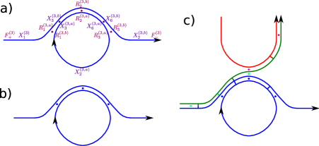
Figure 3:

Figure 4:

Figure 5:

Figure 6:

Figure 7:

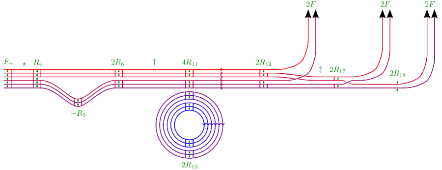
Figure 8:

References

- Wakelam et al. (2006) Wakelam, V., E. Herbst, F. Selsis, and G. Massacrier, 2006. Chemical sensitivity to the ratio of the cosmic-ray ionization rates of He and H2 in dense clouds. Astron. Astrophys 459:813–820.
- Ross and Vlad (1999) Ross, J., and M. O. Vlad, 1999. Nonlinear kinetics and new approaches to complex reaction mechanisms. Annu. Rev. Phys. Chem 50:51–78.
- Papin et al. (2004) Papin, J. A., J. Stelling, N. D. Price, S. Klamt, S. Schuster, and B. O. Palsson, 2004. Comparison of network-based pathway analysis methods. Trends Biotechnol. 22:400–405.
- Pfeiffer et al. (1999) Pfeiffer, T., I. Sánchez-Valdenebro, J. C. Nu o, F. Montero, and S. Schuster, 1999. METATOOL: for studying metabolic networks. Bioinformatics 15:251–257.
- Famili and Palsson (2003) Famili, I., and B. O. Palsson, 2003. The convex basis of the left null space of the stoichiometric matrix leads to the definition of metabolically meaningful pools. Biophys. J. 85:16–26.
- Vallabhajosyula et al. (2006) Vallabhajosyula, R. R., V. Chickarmane, and H. M. Sauro, 2006. Conservation analysis of large biochemical networks. Bioinformatics 22:346–353.
- Klamt et al. (2003) Klamt, S., J. Stelling, M. Ginkel, and E. D. Gilles, 2003. FluxAnalyzer: exploring structure, pathways, and flux distributions in metabolic networks on interactive flux maps. Bioinformatics 19:261–269.
- Meyer (2000) Meyer, C. D., 2000. Matrix Analysis and Applied Linear Algebra, SIAM, Philadelphia, chapter 4, 174.
- William H. Press et al. (1992) William H. Press, S. A. T., W. T. Vetterling, and B. P. Flannery, 1992. Numerical Recipe in C, Cambridge University Press, chapter 2, 36–43. 2nd edition.
- Beard et al. (2004) Beard, D. A., E. Babson, E. Curtis, and H. Qian, 2004. Thermodynamic constraints for biochemical networks. J. Theor. Biol. 228:327–333.
- Coleman and Pothen (1986) Coleman, T. F., and A. Pothen, 1986. The Null Space Problem I. Complexity. SIAM J. Algebraic Discrete Methods 7:527–537.
- Coleman and Pothen (1987) Coleman, T. F., and A. Pothen, 1987. The Null Space Problem II. Algorithms. SIAM J. Algebraic Discrete Methods 8:544–563.
- Berry et al. (1985) Berry, M. W., M. T. Heath, I. Kaneko, M. Lawo, R. J. Plemmons, and R. C. Ward, 1985. An algorithm to compute a sparse basis of the null space. Numer. Math. 47:483–504.
- Gilbert and Heath (1987) Gilbert, J. R., and M. T. Heath, 1987. Computing a Sparse Basis for the Null Space. SIAM J. Algebraic Discrete Methods 8:446–459.