A singular perturbation approach to the steady-state 1D Poisson-Nernst-Planck modeling

Abstract

The reduced 1D Poisson-Nernst-Planck (PNP) model of artificial nanopores in the presence of a permanent charge on the channel wall is studied. More specifically, we consider the limit where the channel length exceed much the Debye screening length and channel’s charge is sufficiently small. Ion transport is described by the nonequillibrium steady-state solution of the PNP system within a singular perturbation treatment. The quantities, $1/\lambda$ – the ratio of the Debye length to a characteristic length scale and $\epsilon$ – the scaled intrinsic charge density, serve as the singular and the regular perturbation parameters, respectively. The role of the boundary conditions is discussed. A comparison between numerics and the analytical results of the singular perturbation theory is presented.

05.60.Cd, 05.40.Jc, 81.07.De

1 Introduction

In many physical situations an exact solution of the full problem could not be obtained, so that various asymptotic and perturbative techniques must be used. Moreover, in many cases, even regular perturbation analysis is useless, and singular perturbation methods must be applied.

An example of such a case constitutes a boundary-layer problem. It is a 1D differential-equation-boundary-value problem on the unit interval for which the highest derivative of the differential equation is multiplied by a small parameter $\delta$:

$$\delta y^{\prime\prime}(x)+c(x)y^{\prime}(x)+d(x)y(x)=f(x),$$ (1)

with the boundary conditions

$$\begin{array}[]{cc}y(0)=a,&y(1)=b.\end{array}$$ (2)

This boundary-value problem is singular because in the limit $\delta\to 0$ one of the solutions abruptly disappears and the limiting solution is not able to satisfy the two boundary conditions in (2). This comes from the fact that by setting $\delta=0$, the order of the differential equation is reduced by 1. One of the method to solve the boundary-value problem (1) and (2) is to look for solutions in the form of series expansion in powers of $\delta$. In order to construct an uniformly and globally valid solution, the interval $0<x<1$ is decomposed into two kinds of regions, an outer region, in which the solution varies slowly as a function of $x$, and an inner region or boundary-layer region, in which the solution varies rapidly as a function of $x$. A boundary-layer region is a narrow region those thickness is typically of order $\delta$ or some power of $\delta$ [1]. One of such boundary value problem is the 1D steady-state PNP system with non-vanishing permanent surface charge on the walls of a nanopore.

Siwy and co-workers reported [2, 3] that ion transport in nanopores with asymmetric fixed charge distributions is characterized by such interesting phenomena as ion current fluctuations, rectification, and pumping. For this reason, we analyse the boundary value problem of the one-dimensional steady-state PNP system with non-vanishing permanent surface charge. Since the conical geometry is experimentally relevant, we consider an uniformly charged conical pore.

The flow of ions through the nanopore caused by an externally applied electric field is analyzed by means of the Nernst-Planck equations together with the Poisson equation, in a self-consistent manner. We are interested in ion transport phenomena occuring in a very long channel i.e. in the limit where the channel length exceed much the channel radii. It justifies the approximation of the channel as a one-dimensional object [4].

The aim of the paper is to show an application of the singular perturbation theory to such one-dimensional PNP systems where the following quantities - the ratio of the Debye length $\xi_{\rm{D}}$ to the channel length $L$, denoted as $1/\lambda\sim\xi_{\rm{D}}/L$, and the channel surface charge $\sigma$ - serve as the perturbation parameters. The system can be viewed as a singularly perturbed problem in $1/\lambda$ and a regularly perturbed in $\epsilon$ that denotes a dimensionless scaled surface charge density. In the long channel limit, we analyzed the leading term in $1/\lambda$, while $\epsilon$ is considered as the regular expansion parameter. In our approach, we make use of above-described method to construct an uniformly and globally valid solution by calculating separately the outer and inner solutions and matching them then in a smooth manner.

2 Ion Transport

2.1 One dimensional Poisson-Nernst -Planck (PNP)

In this paper we study ion transport through a long conical nanopore of the length $L=1$ (scaling of the $z$-coordinate by the channel length $L$, whereas the radial coordinate $r$ is scaled by the small opening radius $R(0)$) with uniformly charged wall, cf. Fig. 1. The ion flow through the charged conical nanopore could be driven by the ion concentration gradients and by the electric field modeled together by means of the electrodiffusion equation. Diffusion in orthogonal direction of the pore is confined to a channel of variable area of $\pi R^{2}(z)$ (see Fig. 1). The electric field inside the pore is in turn governed by applied field and by the ion concentrations through the Poisson equation. We are interested in the non-equillibrium steady-state ion flux and electrical current which can persist either due to applied voltage or due to a concentration gradient.

Figure 1: Schema of the section of the conical channel. The channel’s wall is uniformly charged with surface charge density $\sigma$. The local radius of the cone $R(z)$, is given by Eq. 4.

One can reduce the problem from 3D to 1D assuming instantaneous equillibration in the transverse direction

$$\begin{array}[]{cc}\bar{c}(z,t)\approx c(z,r,t)\mathcal{A}(z),{}{}&\Phi(z,t)\approx\Phi(z,r,t),\end{array}$$ (3)

where

$$\begin{array}[]{cc}\mathcal{A}(z)=\pi R^{2}(z),{}{}&R(z)=(1+\gamma z)\end{array}$$ (4)

with $\gamma=R(1)-1$ denoting a scaled slope of the cone’s radius, with the scaling of the radial coordinate $r$ by $R(0)$.

The 3D PNP equations for steady state ion currents $I_{\rm{K}^{+}}$ and $I_{\rm{Cl}^{-}}$ thus become in the 1D approximation (cf. Ref. [4] and Appendix A):

$$\begin{array}[]{cc}\vspace{10pt}\displaystyle-I_{\mathrm{K^{+}}}=\frac{d}{dz}\bar{c}_{\mathrm{K^{+}}}(z)+\bar{c}_{\mathrm{K^{+}}}(z)\frac{d\Phi(z)}{dz}-\bar{c}_{\mathrm{K^{+}}}(z)\frac{2}{R(z)}\frac{dR(z)}{dz},\\ \displaystyle I_{\mathrm{Cl^{-}}}=\frac{d}{dz}\bar{c}_{\mathrm{Cl^{-}}}(z)-\bar{c}_{\mathrm{Cl^{-}}}(z)\frac{d\Phi(z)}{dz}-\bar{c}_{\mathrm{Cl^{-}}}(z)\frac{2}{R(z)}\frac{dR(z)}{dz},\end{array}$$ (5)

together with the reduced Poisson equation

$$\frac{d^{2}\Phi(z)}{dz^{2}}+\frac{2}{R(z)}\frac{dR(z)}{dz}\frac{d\Phi(z)}{dz}=-\lambda^{2}\frac{\epsilon}{R(z)}-\lambda^{2}\frac{1}{\pi R^{2}(z)}\left(\bar{c}_{\mathrm{K^{+}}}(z)-\bar{c}_{\mathrm{Cl^{-}}}(z)\right),$$ (6)

where

$$\frac{1}{\lambda}=\displaystyle\sqrt{\frac{\epsilon_{0}\epsilon_{w}k_{\rm B}TR^{2}(0)}{\rm{e}^{2}c_{0}N_{\rm{A}}L^{2}}}=\sqrt{2c}\left(\frac{\xi_{\rm{D}}}{L}\right),$$ (7)

is the scaled Debye screening length, and the effective dimensionless surface charge density reads

$$\epsilon=\frac{2\sigma R(0)}{\rm{e}c_{0}N_{\rm A}}.$$ (8)

In Eq. (7), $c$ denotes dimensionless concentration (see the definition given by Eq. (10)), $\xi_{\rm{D}}=\left[\epsilon_{0}\epsilon_{w}k_{\rm{B}}T/(2\rm{e}^{2}N_{\rm{A}}10^{3}c_{\rm{bulk}})\right]^{(1/2)}$ (in meters) is the Debye length in bulk (see Ref. [4, 5]), $\epsilon_{0}$ the dielectrical constant of vacuum, $\epsilon_{w}\approx 80$ the relative dielectrical constant of water, $k_{\rm{B}}$ the Boltzmann constant, $T$ the temperature, $\rm{e}$ the elementary charge, $N_{\rm{A}}$ the Avogadro number, $c_{\rm{bulk}}$ the bulk concentration of ions, and $c_{0}$ is an arbitrary reference 1D-concentration (in $1/6.023\times 10^{-14}$ moles/m). Note that the coordinate $z$ is also dimensionless in the above equations (measured in units of $L$).

2.2 Rigorous Boundary Conditions

The boundary conditions are

$$\begin{array}[]{cc}\vspace{10pt}\bar{c}_{\mathrm{K^{+}}}(0)=\pi c_{\mathrm{K^{+},L}},&\bar{c}_{\mathrm{Cl^{-}}}(0)=\pi c_{\mathrm{Cl^{-},L}},\\ \vspace{10pt}\bar{c}_{\mathrm{K^{+}}}(1)=\pi(1+\gamma)^{2}c_{\mathrm{K^{+},R}},&\bar{c}_{\mathrm{Cl^{-}}}(1)=\pi(1+\gamma)^{2}c_{\mathrm{Cl^{-},R}},\\ \Phi(0)=0,&\Phi(1)=\Phi_{\mathrm{R}},\end{array}$$ (9)

wherein

$$c_{i,\{\mathrm{L,R}\}}=10^{3}c_{\mathrm{bulk},\{\mathrm{L,R}\}}R^{2}(0)/c_{0},~{}~{}~{}\rm{i=K}^{+},~{}\rm{Cl}^{-}$$ (10)

and $c_{\mathrm{bulk},\{\mathrm{L,R}\}}$ denote the bulk concentrations of ions on the left and right sides (in moles), respectively. The electro-neutrality condition yields: $c_{\mathrm{K^{+},L}}=c_{\mathrm{Cl^{-},L}}=c_{\mathrm{L}}$, and $c_{\mathrm{K^{+},R}}=c_{\mathrm{Cl^{-},R}}=c_{\mathrm{R}}$. Furthermore, the difference of dimensionless potentials across the nanopore is related to the applied voltage $U$ (in units of Volts) by $\Phi(0)-\Phi(1)=\mathrm{e}U/(k_{\mathrm{B}}T)$, yielding $U=-k_{\rm{B}}T\Phi(1)/\rm{e}$.

3 Singular perturbation study

3.1 Perturbation parameters

The coresponding system contains two small parameters. The first one $1/\lambda$ is related to the ratio of the Debye length to a characteristic length scale. Assuming that $\lambda\to\infty$ we search for an aproximate solution of equations (5) and (6) in the form

$$\begin{array}[]{c}\vspace{10pt}\displaystyle\Phi(z)=\Phi^{(0)}(z)+\frac{1}{\lambda}\Phi^{(1)}(z)+\dots,\\ \vspace{10pt}\displaystyle\bar{c}_{\mathrm{K^{+}}}(z)=c_{\mathrm{K^{+}}}^{(0)}(z)+\frac{1}{\lambda}c_{\mathrm{K^{+}}}^{(1)}(z)+\dots,\\ \displaystyle\bar{c}_{\mathrm{Cl^{-}}}(z)=c_{\mathrm{Cl^{-}}}^{(0)}(z)+\frac{1}{\lambda}c_{\mathrm{Cl^{-}}}^{(1)}(z)+\dots.\end{array}$$ (11)

The second small parameter corresponds to the re-scaled intrinsic charge density $\epsilon$ (see in Eq. 8). Furthermore, we represent $\Phi^{(i)}(z),c_{\mathrm{K^{+}}}^{(i)}(z),c_{\mathrm{Cl^{-}}}^{(i)}(z)$ as a series in $\epsilon$

$$\begin{array}[]{c}\vspace{10pt}\displaystyle\Phi^{(i)}(z)=\Phi^{(i)}_{(0)}(z)-\epsilon\Phi^{(i)}_{(1)}(z)+\dots,\\ \vspace{10pt}\displaystyle\bar{c}_{\mathrm{K^{+}}}^{(i)}(z)=c_{\mathrm{K^{+}},~{}{(0)}}^{(i)}(z)-\epsilon c_{\mathrm{K^{+}},~{}{(1)}}^{(i)}(z)+\dots,\\ \displaystyle\bar{c}_{\mathrm{Cl^{-}}}^{(i)}(z)=c_{\mathrm{Cl^{-}},~{}{(0)}}^{(i)}(z)-\epsilon c_{\mathrm{Cl^{-}},~{}{(1)}}^{(i)}(z)+\dots.\end{array}$$ (12)

where $i=0,1,\dots$. Finally, a singularly perturbated boundary – value problem in two independent perturbation parameters $1/\lambda$ and $\epsilon$ is obtained. We search for the solution letting $1/\lambda\to 0$, while $\epsilon$ is considered as the expansion parameter. Note that the perturbation problem is singular in $1/\lambda$ and regular in $\epsilon$.

3.2 The outer expansion.

These series are obtained by holding $z$ fixed and letting $1/\lambda\to 0$. In zeroth order in $1/\lambda$, the problem reduces to

$$\left(c^{(0)}_{\rm{K}^{+}}(z)-c^{(0)}_{\rm{Cl}^{-}}(z)\right)/\pi R^{2}(z)=-\frac{\epsilon}{R(z)},$$ (13)

reflecting the charge neutrality in the interior, and

$$\begin{array}[]{c}\vspace{20pt}\displaystyle-I^{(0)}_{\rm{K}^{+}}=\frac{d}{dz}c^{(0)}_{\rm{K}^{+}}(z)-2\frac{R^{\prime}(z)}{R(z)}c^{(0)}_{\rm{K}^{+}}(z)+\frac{d\Phi^{(0)}(z)}{dz}c^{(0)}_{\rm{K}^{+}}(z),\\ \displaystyle I^{(0)}_{\rm{Cl}^{-}}=\frac{d}{dz}c^{(0)}_{\rm{Cl}^{-}}(z)-2\frac{R^{\prime}(z)}{R(z)}c^{(0)}_{\rm{Cl}^{-}}(z)-\frac{d\Phi^{(0)}(z)}{dz}c^{(0)}_{\rm{Cl}^{-}}(z).\end{array}$$ (14)

Adding and substracting the current formulas, we obtain

$$\begin{array}[]{c}\vspace{10pt}\displaystyle-I^{(0)}_{\rm{K}^{+}}+I^{(0)}_{\rm{Cl}^{-}}=\frac{d}{dz}\left(c^{(0)}_{\rm{K}^{+}}(z)+c^{(0)}_{\rm{Cl}^{-}}(z)\right)\\ \vspace{10pt}\displaystyle-2\frac{R^{\prime}(z)}{R(z)}\left(c^{(0)}_{\rm{K}^{+}}(z)+c^{(0)}_{\rm{Cl}^{-}}(z)\right)-\frac{d\Phi^{(0)}}{dz}\epsilon\pi R(z),\\ \displaystyle-\left(I^{(0)}_{\rm{K}^{+}}+I^{(0)}_{\rm{Cl}^{-}}\right)=-\epsilon\pi R^{\prime}(z)+\frac{d\Phi^{(0)}}{dz}\left(c^{(0)}_{\rm{K}^{+}}(z)+c^{(0)}_{\rm{Cl}^{-}}(z)\right),\end{array}$$ (15)

where $-I^{(0)}_{\rm{K}^{+}}+I^{(0)}_{\rm{Cl}^{-}}=J^{(0)}=\rm{const}$, $I^{(0)}_{\rm{K}^{+}}+I^{(0)}_{\rm{Cl}^{-}}=I^{(0)}=\rm{const}$. The both sorts of ions have equal diffusion coefficients (see Ref. [6]), i.e. $D_{\mathrm{\rm{K}^{+}}}=D_{\mathrm{\rm{Cl}^{-}}}=D$, thus $J^{(0)}$ yields an approximation to the negative of the total mass current, whereas $I^{(0)}$ approximates the total electric current (see also Ref. [7]),

$$\begin{array}[]{c}\vspace{20pt}\displaystyle\pi\epsilon R(z)\frac{d\Phi^{(0)}(z)}{dz}=-J^{(0)}+\frac{d}{dz}\left(c^{(0)}_{\rm{K}^{+}}(z)+c^{(0)}_{\rm{Cl}^{-}}(z)\right)\\ \vspace{10pt}\displaystyle-2\frac{R^{\prime}(z)}{R(z)}\left(c^{(0)}_{\rm{K}^{+}}(z)+c^{(0)}_{\rm{Cl}^{-}}(z)\right),\\ \displaystyle\left(c^{(0)}_{\rm{K}^{+}}(z)+c^{(0)}_{\rm{Cl}^{-}}(z)\right)\frac{d\Phi^{(0)}(z)}{dz}=-I^{(0)}+\pi\epsilon R^{\prime}(z).\end{array}$$ (16)

Then one gets

$$\begin{array}[]{c}\vspace{10pt}\displaystyle\left(c^{(0)}_{\rm{K}^{+}}(z)+c^{(0)}_{\rm{Cl}^{-}}(z)\right)\bigg{(}J^{(0)}-\frac{d}{dz}\left(c^{(0)}_{\rm{K}^{+}}(z)+c^{(0)}_{\rm{Cl}^{-}}(z)\right)\\ \vspace{10pt}\displaystyle+2\frac{R^{\prime}(z)}{R(z)}\left(c^{(0)}_{\rm{K}^{+}}(z)+c^{(0)}_{\rm{Cl}^{-}}(z)\right)\bigg{)}=\displaystyle\pi\epsilon R(z)\left(I^{(0)}-\pi\epsilon R^{\prime}(z)\right).\end{array}$$ (17)

One cannot find exact solution to this differential equation. It is solved perturbatively in $\epsilon$ with the solution approximated as

$$\begin{array}[]{c}\vspace{10pt}\displaystyle\left(c^{(0)}_{\rm{K}^{+}}(z)+c^{(0)}_{\rm{Cl}^{-}}(z)\right)=c^{(0)}_{\Sigma}(z)=c^{(0)}_{\Sigma,(0)}(z)-\epsilon c^{(0)}_{\Sigma,(1)}(z)+\dots\\ \Phi^{(0)}(z)=\Phi^{(0)}_{(0)}(z)-\epsilon\Phi^{(0)}_{(1)}(z)+\dots,\end{array}$$ (18)

where the upper index denotes the order of expansion in $1/\lambda$, and the lower one in $\epsilon$.

3.3 The boundary layer solutions.

Let $\delta(1/\lambda)$ be the width of the boundary layer which is a function of $1/\lambda$. The problem is rescaled near $z=0$ by setting $\zeta=z/\delta(1/\lambda)$. It has been found that $\delta(1/\lambda)=1/\lambda$ and for $z$ in the boundary layer, $\zeta=O(1)$. Thus, we introduce the stretched coordinate

$$\zeta=\lambda z,$$ (19)

where $\zeta\in[0,+\infty)$ and express the concentrations and the electric potential in terms of this coordinate as

$$\begin{array}[]{c}\vspace{10pt}\displaystyle c_{\rm{K}^{+}}(\zeta/\lambda;1/\lambda)=\displaystyle p(\zeta;1/\lambda),\\ \vspace{10pt}\displaystyle c_{\rm{Cl}^{-}}(\zeta/\lambda;1/\lambda)=\displaystyle n(\zeta;1/\lambda),\\ \displaystyle\Phi(\zeta/\lambda;1/\lambda)=\displaystyle\phi(\zeta;1/\lambda).\end{array}$$ (20)

In the right boundary layer, i.e. near $z=1$ we set the another stretched variable

$$\chi=\lambda(z-1),$$ (21)

where $\chi\in(-\infty,0]$ and define analogously

$$\begin{array}[]{c}\vspace{10pt}\displaystyle c_{\rm{K}^{+}}(\chi/\lambda+1;1/\lambda)=\displaystyle\tilde{p}(\chi;1/\lambda),\\ \vspace{10pt}\displaystyle c_{\rm{Cl}^{-}}(\chi/\lambda+1;1/\lambda)=\displaystyle\tilde{n}(\chi;1/\lambda),\\ \displaystyle\Phi(\chi/\lambda+1;1/\lambda)=\displaystyle\tilde{\phi}(\chi;1/\lambda).\end{array}$$ (22)

Each of these functions is written as an asymptotic series, namely,

$$\begin{array}[]{cc}\vspace{10pt}\displaystyle p(\zeta;1/\lambda)=p^{(0)}(\zeta)+\frac{1}{\lambda}p^{(1)}(\zeta)+\dots,&~{}~{}\displaystyle\tilde{p}(\chi;1/\lambda)=\tilde{p}^{(0)}(\chi)+\frac{1}{\lambda}\tilde{p}^{(1)}(\chi)+\dots,\\ \vspace{10pt}\displaystyle n(\zeta;1/\lambda)=n^{(0)}(\zeta)+\frac{1}{\lambda}n^{(1)}(\zeta)+\dots,&~{}~{}\displaystyle\tilde{n}(\chi;1/\lambda)=\tilde{n}^{(0)}(\chi)+\frac{1}{\lambda}\tilde{n}^{(1)}(\chi)+\dots,\\ \displaystyle\phi(\zeta;1/\lambda)=\phi^{(0)}(\zeta)+\frac{1}{\lambda}\phi^{(1)}(\zeta)+\dots,&~{}~{}\displaystyle\tilde{\phi}(\chi;1/\lambda)=\tilde{\phi}^{(0)}(\chi)+\frac{1}{\lambda}\tilde{\phi}^{(1)}(\chi)+\dots,\end{array}$$ (23)

and

$$\begin{array}[]{cc}\vspace{10pt}\displaystyle R(\zeta)\to 1,&\quad R(\chi)\to 1+\gamma.\end{array}$$ (24)

The upper indixes correspond to the order of the expansion in $1/\lambda$. The limit expansions is obtained by holding $\zeta$ and $\chi$ fixed and letting $1/\lambda\to 0$.

In turn, each of the $p^{(0)}(\zeta),n^{(0)}(\zeta),\phi^{(0)}(\zeta)$ functions is written as an asymptotic series in $\epsilon$, namely,

$$\begin{array}[]{cc}\vspace{10pt}\displaystyle p^{(0)}(\zeta)=p^{(0)}_{(0)}(\zeta)-\epsilon p^{(0)}_{(1)}(\zeta)+\dots,&\quad\displaystyle\tilde{p}^{(0)}(\chi)=\tilde{p}^{(0)}_{(0)}(\chi)-\epsilon\tilde{p}^{(0)}_{(1)}(\chi)+\dots,\\ \vspace{10pt}\displaystyle n^{(0)}(\zeta)=n^{(0)}_{(0)}(\zeta)-\epsilon n^{(0)}_{(1)}(\zeta)+\dots,&\quad\displaystyle\tilde{n}^{(0)}(\chi)=\tilde{n}^{(0)}_{(0)}(\chi)-\epsilon\tilde{n}^{(0)}_{(1)}(\chi)+\dots,\\ \displaystyle\phi^{(0)}(\zeta)=\phi^{(0)}_{(0)}(\zeta)-\epsilon\phi^{(0)}_{(1)}(\zeta)+\dots,&\quad\displaystyle\tilde{\phi}^{(0)}(\chi)=\tilde{\phi}^{(0)}_{(0)}(\chi)-\epsilon\tilde{\phi}^{(0)}_{(1)}(\chi)+\dots.\end{array}$$ (25)

The lower indixes refer to the order of the series expansion in $\epsilon$. In the leading order functions in $1/\lambda$ the transport equations read

$$\begin{array}[]{cc}\vspace{20pt}\displaystyle 0=\frac{d}{d\zeta}p^{(0)}(\zeta)+\frac{d\phi^{(0)}(\zeta)}{d\zeta}p^{(0)}(\zeta),&\quad\displaystyle 0=\frac{d}{d\chi}\tilde{p}^{(0)}(\chi)+\frac{d\tilde{\phi}^{(0)}(\chi)}{d\chi}\tilde{p}^{(0)}(\chi),\\ \displaystyle 0=\frac{d}{d\zeta}n^{(0)}(\zeta)-\frac{d\phi^{(0)}(\zeta)}{d\zeta}n^{(0)}(\zeta),&\quad\displaystyle 0=\frac{d}{d\chi}\tilde{n}^{(0)}(\chi)-\frac{d\tilde{\phi}^{(0)}(\chi)}{d\chi}\tilde{n}^{(0)}(\chi),\end{array}$$ (26)

together with the Poisson equation

$$\begin{array}[]{c}\vspace{10pt}\displaystyle\frac{1}{\pi}\left(p^{(0)}(\zeta)-n^{(0)}(\zeta)\right)+\epsilon=-\frac{d^{2}\phi^{(0)}(\zeta)}{d\zeta^{2}},\\ \displaystyle\frac{1}{\pi(1+\gamma)^{2}}\left(\tilde{p}^{(0)}(\chi)-\tilde{n}^{(0)}(\chi)\right)+\frac{\epsilon}{1+\gamma}=-\frac{d^{2}\tilde{\phi}^{(0)}(\chi)}{d\chi^{2}},\end{array}$$ (27)

and obeys the following boundary conditions

$$\begin{array}[]{cccc}\vspace{10 pt}p^{(0)}_{(0)}(0)=\pi c_{\mathrm{L}},&p^{(0)}_{(i)}(0)=0,&\quad\tilde{p}^{(0)}_{(0)}(0)=\pi(1+\gamma)^{2}c_{\mathrm{R}},&\tilde{p}^{(0)}_{(i)}(0)=0,\\ \vspace{10pt}n^{(0)}_{(0)}(0)=\pi c_{\mathrm{L}},&n^{(0)}_{(i)}(0)=0,&\quad\tilde{n}^{(0)}_{(0)}(0)=\pi(1+\gamma)^{2}c_{\mathrm{R}},&\tilde{n}^{(0)}_{(i)}(0)=0,\\ \phi^{(0)}_{(0)}(0)=0,&\phi^{(0)}_{(i)}(0)=0,&\quad\tilde{\phi}^{(0)}_{(0)}(0)=\Phi_{\mathrm{R}},&\tilde{\phi}^{(0)}_{(i)}(0)=0,\end{array}$$ (28)

with $i=1,2,\dots$. As a next step, we integrate the left boundary layer of the Nernst-Planck equations (26)

$$\begin{array}[]{cc}\vspace{10pt}\displaystyle p^{(0)}(\zeta)=p^{(0)}_{(0)}(0)e^{-\phi^{(0)}_{(0)}(\zeta)}\left\{1+\epsilon\phi^{(0)}_{(1)}(\zeta)+\epsilon^{2}\left(-\phi^{(0)}_{(2)}(\zeta)+\frac{1}{2}\phi^{(0)2}_{(1)}(\zeta)\right)\right\}+O(\epsilon^{3}),\\ \displaystyle n^{(0)}(\zeta)=n^{(0)}_{(0)}(0)e^{\phi^{(0)}_{(0)}(\zeta)}\left\{1-\epsilon\phi^{(0)}_{(1)}(\zeta)+\epsilon^{2}\left(\phi^{(0)}_{(2)}(\zeta)+\frac{1}{2}\phi^{(0)2}_{(1)}(\zeta)\right)\right\}+O(\epsilon^{3}).\end{array}$$ (29)

After the substitution $\{p,n,\phi\}\to\{\tilde{p},\tilde{n},\tilde{\phi}\}$ in the equations (29), we obtain the right boundary layer solutions. Then, we put these expressions for the concentrations into the Poisson equation (27).

3.4 Matching procedure.

Now a matching of these two representations is needed. So we choose constants to make left (right) boundary layer solutions and outer expansion, respectively, coincide for each order of $\epsilon$ (as $1/\lambda\to 0$) in some intermediate zone between the left (right) boundary layer and the outer region, respectively. Furthemore, in the left intermediate zone an intermediate variable $z_{\alpha}$ is introduced, where

$$z_{\alpha}=\left\{\begin{array}[]{c}\vspace{10pt}(1/\lambda)^{-\alpha}z,\\ (1/\lambda)^{1-\alpha}\zeta,\end{array}\right.$$ (30)

and $0<\alpha<1$ such as

$$\begin{array}[]{c}\vspace{10pt}\displaystyle\lim\frac{\zeta}{z_{\alpha}}\to\infty~{}~{}\rm{when}~{}~{}\frac{1}{\lambda}\to 0,\\ \displaystyle\lim\frac{z}{z_{\alpha}}\to 0~{}~{}\rm{when}~{}~{}\frac{1}{\lambda}\to 0.\end{array}$$ (31)

The above-described procedure is also applied to find an intermediate variable ($z_{\beta}-1=(1/\lambda)^{1-\beta}\chi$) in the right intermediate zone. The ensuing conditions are ($z_{\alpha},z_{\beta}~{}\rm{fixed~{}and}~{}1/\lambda\to 0$)

$$\begin{array}[]{cc}\vspace{10pt}\displaystyle c^{(0)}_{\rm{K}^{+}}(0)=p^{(0)}(\infty),&\quad c^{(0)}_{\rm{K}^{+}}(1)=\tilde{p}^{(0)}(-\infty),\\ \vspace{10pt}c^{(0)}_{\rm{Cl}^{-}}(0)=n^{(0)}(\infty),&\quad c^{(0)}_{\rm{Cl}^{-}}(1)=\tilde{n}^{(0)}(-\infty),\\ \Phi^{(0)}(0)=\phi^{(0)}(\infty),&\quad\Phi^{(0)}(1)=\tilde{\phi}^{(0)}(-\infty),\end{array}$$ (32)

and

$$\begin{array}[]{cc}\displaystyle\frac{d\phi^{(0)}}{d\zeta}(\infty)=0,&\quad\displaystyle\frac{d\tilde{\phi}^{(0)}}{d\chi}(-\infty)=0.\end{array}$$ (33)

Adding and substracting the formulas (13) and (52), (13) and (57), respectively, we obtain

$$c^{(0)}_{(i),\{\mathrm{K^{+},Cl^{-}}\}}(0)=\frac{1}{2}c^{(0)}_{(i),\Sigma}(0)\pm\left\{\begin{array}[]{cc}\vspace{10pt}\displaystyle\frac{\pi}{2}&\rm{for,i=1}\\ \displaystyle 0&\rm{for,i=0,2,3,\dots}\end{array}\right.$$ (34)

where the upper sign refers to K⁺ ions and the lower one to Cl^-. To find the values of $\phi^{(0)}(\infty)$, we make use of

$$\frac{1}{\pi}\left(p^{(0)}(\infty)-n^{(0)}(\infty)\right)+\epsilon=0.$$ (35)

Taking into account the matching conditions (32) together with (34) we get conditions for unknown constants $J^{(0)}_{(i)},I^{(0)}_{(i)},C^{(0)}_{(i)},E^{(0)}_{(i)}$, where $i=0,1,2,\dots$

The above procedure allows us to find matching conditions between the outer expansion and the right boundary layer as well.

3.5 The Poisson equation in the boundary layers.

Now we consider the Poisson equation (27) within the boundary layer, and integrate them following the Ref. [7]. We are able to find analytical solutions of (27) up to the second order in $\epsilon$. The solutions of the Poisson equation (27) depend on the boundary conditions. For $c_{\rm{K}^{+},L}=c_{\rm{Cl}^{-},L}$, $\phi^{(0)}_{(0)}(\zeta)=0$ (see also Ref. [7]), $\displaystyle\phi^{(0)}_{(1)}(\zeta)=\frac{1}{2c_{L}}\left(e^{-\sqrt{2c_{L}}\zeta}-1\right)$, and $\phi^{(0)}_{(2)}(\zeta)=0$.

Similar results hold for the solutions in the right boundary layer. If $c_{\rm{K}^{+},R}=c_{\rm{Cl}^{-},R}$, then $\tilde{\phi}^{(0)}_{(0)}(\chi)=\Phi_{R}$ (as in Ref. [7]),
$\displaystyle\tilde{\phi}^{(0)}_{(1)}(\chi)=\frac{1}{2c_{R}(1+\gamma)}\left(e^{\sqrt{2c_{L}}\chi}-1\right)$, and $\tilde{\phi}^{(0)}_{(2)}(\chi)=0$.

3.6 Uniformly valid solutions.

To obtain an approximation that is valid uniformly on $[0,1]$, we add the boundary and outer appoximations and subtract their common limit in the intermediate zone. Thus, we find:

$$\vspace{10pt}\Phi(z)=\Phi^{(0)}_{(0)}(z) - \epsilon\bigg{\{}\phi^{(0)}_{(1)}(\lambda z)+\Phi^{(0)}_{(1)}(z)+\tilde{\phi}^{(0)}_{(1)}(\lambda(1-z))$$ (36)

$$+ \displaystyle\frac{1}{2c_{\mathrm{L}}}+\displaystyle\frac{1}{2c_{\mathrm{R}}(1+\gamma)}\bigg{\}}+O(\epsilon^{2}),$$

$$\vspace{10pt}\displaystyle\bar{c}_{\{\mathrm{K^{+},Cl^{-}}\}}(z) = \frac{1}{2}c^{(0)}_{\Sigma,(0)}(z)-\frac{1}{2}\epsilon\bigg{\{}\pm\pi R(z)+c^{(0)}_{\Sigma,(1)}(z)\mp 2\pi c_{\mathrm{L}}\phi^{(0)}_{(1)}(\lambda z)$$ (37)

$$\mp 2\pi c_{\mathrm{R}}(1+\gamma)^{2}\tilde{\phi}^{(0)}_{(1)}(\lambda(1-z))\mp\pi(2+\gamma)\bigg{\}}+O(\epsilon^{2}),$$

where the upper sign refers to K⁺ ions and the lower one to Cl^-.

4 The Donnan boundary conditions

Approximatively, one can impose the so-called Donnan equilibrium boundary conditions at the channel ends [8], reading:

$$\vspace{10pt}\displaystyle\bar{c}^{\mathrm{Don}}_{i}(z_{\{\mathrm{L,R}\}})=\frac{10^{3}\pi R(z_{\{\mathrm{L,R}\}})^{2}}{2c_{0}}\Big{(}-\nu_{i}X_{\{\mathrm{L,R}\}}+\sqrt{X^{2}_{\{\mathrm{L,R}\}}+4c^{2}_{\mathrm{bulk},\{\mathrm{L,R}\}}}\Big{)},$$ (38)

$$\displaystyle\Phi^{\mathrm{Don}}(z_{\{\mathrm{L,R}\}})=\Phi_{\{\mathrm{L,R}\}}-\frac{1}{\nu_{i}}\ln\frac{\bar{c}^{\mathrm{Don}}_{i}(z_{\{\mathrm{L,R}\}})c_{0}}{10^{3}\pi R(z_{\{\mathrm{L,R}\}})^{2}c_{\mathrm{bulk}}(z_{\{\mathrm{L,R}\}})},$$ (39)

where $\displaystyle X_{\{\mathrm{L,R}\}}=\displaystyle\frac{2\sigma}{F}\times\frac{1}{R(z_{\{\mathrm{L,R}\}})}$ (in M) and i = K⁺, Cl^-. Here, $R(z_{\{\mathrm{L,R}\}})$ denotes the nanopore radii at the left and right ends of the pore, respectively.

Let us expand the Donnan equilibrium conditions in terms of power of $\epsilon$ and afterwards, using the definition of $c_{i,{\{\mathrm{L,R}\}}}$, i = K⁺, Cl^- (see Sec. Rigorous Boundary Conditions), we find our dimensionless functions at both channel ends

$$\begin{array}[]{c}\vspace{10pt}\displaystyle\bar{c}^{\rm{Don}}_{i}(z_{\{\mathrm{L,R}\}})=\pi R(z_{\{\mathrm{L,R}\}})^{2}c_{i}\mp\frac{\pi}{2}R(z_{\{\mathrm{L,R}\}})\epsilon\\ \vspace{10pt}\displaystyle+\frac{\pi}{8c_{i}}\epsilon^{2}-\frac{\pi}{128c^{3}_{i}R(z_{\{\mathrm{L,R}\}})^{2}}\epsilon^{4}+\dots,\\ \displaystyle\Phi^{\rm{Don}}(z_{\{\mathrm{L,R}\}})=\Phi_{\{\mathrm{L,R}\}}+\frac{1}{2c_{i}R(z_{\{\mathrm{L,R}\}})}\epsilon\\ \vspace{10pt}\displaystyle-\frac{1}{48c^{3}_{i}R(z_{\{\mathrm{L,R}\}})^{3}}\epsilon^{3}+\frac{3}{1280c^{5}_{i}R(z_{\{\mathrm{L,R}\}})^{5}}\epsilon^{5}+\dots,\\ \end{array}$$ (40)

where the upper sign in $\bar{c}^{\rm{Don}}_{i}(z_{\{\mathrm{L,R}\}})$ refers to potassium ions and the lower one to chloride, $i=\rm{K}^{+},\rm{Cl}^{-}$, $z_{\mathrm{L}}=1$, and $z_{\mathrm{R}}=(1+\gamma)$. Note that the Donnan equilibrium conditions (Eq. (20)-(21) in Ref. [8]) have been obtained under the assumption of local electroneutrality at the channel borders.

Theorem 1

Let $1/\lambda\to 0$. If $\zeta\to+\infty$, then the left boundary layer solutions $p^{(0)}(\zeta),n^{(0)}(\zeta),\phi^{(0)}(\zeta)$ given by an asymptotic series (25) tend to the Donnan asymptotic series (LABEL:Donnan) in $z_{L}$.

One can formulate analogue of above theorem for right boundary layer solutions.

Proof: We first observe that the solution of the following transport equation

$$\displaystyle-I^{(0)}_{p} = \frac{d}{d\zeta}p^{(0)}(\zeta)+\frac{d\phi^{(0)}}{d\zeta}p^{(0)}(\zeta),\quad\quad\zeta\in[0,+\infty),$$ (41)

$$\displaystyle I^{(0)}_{n} = \frac{d}{d\zeta}n^{(0)}(\zeta)-\frac{d\phi^{(0)}}{d\zeta}n^{(0)}(\zeta),$$ (42)

when $\displaystyle I^{(0)}_{\{p,n\}}\to 0$ (the equilibrium condition) tends to the Boltzmann distribution:

$$p^{(0)}(\zeta) \to p^{(0)}(0)e^{-(\phi^{(0)}(\zeta)-\phi^{(0)}(0))},$$ (43)

$$n^{(0)}(\zeta) \to n^{(0)}(0)e^{(\phi^{(0)}(\zeta)-\phi^{(0)}(0))}.$$ (44)

It gives us the Donnan equilibrium condition for a given potential drop. On the other hand, it is known from the matching procedure that $p^{(0)}(\zeta)$, $n^{(0)}(\zeta)$, $\phi^{(0)}(\zeta)$ when $\zeta\to+\infty$ must tend to the outer expansions $\bar{c}^{(0)}_{\rm{K}^{+}}(0)$, $\bar{c}^{(0)}_{\rm{Cl}^{-}}(0)$, $\Phi^{(0)}(0)$. This means that for $\zeta\to+\infty$ the condition of local electroneutrality is fulfilled. And then we end up with series given by Eqs. (LABEL:Donnan).

In turn, the outer solutions $\bar{c}^{(0)}_{\rm{K}^{+}}(z)$, $\bar{c}^{(0)}_{\rm{Cl}^{-}}(z)$, $\Phi^{(0)}(z)$ (given by (37) and (36)) tend to the Donnan asymptotic series (LABEL:Donnan) for $z=z_{\{\mathrm{L,R}\}}$, respectively. Thus, on the basis of Theorem 1 and the matching procedure, one can formulate

Theorem 2

If $1/\lambda\to 0$, then the outer expansions $\bar{c}^{(0)}_{\rm{K}^{+}}(z),\bar{c}^{(0)}_{\rm{Cl}^{-}}(z),\Phi^{(0)}(z)$ approximate the solutions of the 1D-PNP system (Eq. (6) and (5)) with the Donnan boundary conditions satisfying the local electroneutrality at the boundaries.

Proof:

The boundary layer solutions calculated with the Donnan boundary conditions (LABEL:Donnan) (after inversion to normal coordinate $z$) are restricted to the points at the boundaries approximated by these series (LABEL:Donnan).

The above-presented theorem was already demonstrated in Ref. [9], in which a singular perturbation expansion was also used to derive the Donnan potential. We recall this finding, however, in a different manner. One can conclude that in the limit where the channel length exceeds much the Debye screening length, the Donnan jumps at the channel borders can be safely used instead of the rigorous treatment of the the boundary layers of finite width.

Moreover, on the basis of the matching conditions given by (32) and Theorem 1, we notice that unknown constants (present in the outer approximation), in particular the total flux $J^{(0)}$ and the electric current $I^{(0)}$, in both discussed cases of boundary conditions constitute the same series in $\epsilon$.

5 Results

5.1 Perturbation vs. numerics

We shall present a comparison of the analytical results calculated by the above-described singular perturbation method with numerical solutions. The 1D PNP system (equations (5)-(6)), with boundary conditions (equations in (9)), is integrated numerically by making use of a collocating method with adaptive meshing [10]. We choose the following set of parameters: $R(0)=3$ nm, $R(1)=6.616$ nm, $L=200$ nm, $\gamma=1.2055$, the room temperature ($T=298$ K), the relative dielectric constant of water $\epsilon_{w}=80$, and the diffusion coefficients of the ions $D_{\rm{K}^{+}}=D_{\rm{Cl}^{-}}=2\times 10^{9}$ nm²/s [6]. For such a channel, the value of the first perturbation parameter $1/\lambda$ is about $10^{-2}$. The square of this parameter is sufficiently small. However, this is not enough to provide a good approximation to the PNP system with a varying value of the surface charge density which is not that small in the reality. To test the limits of regular perturbation method with respect to the second expansion parameter $\epsilon$, we consider the two different cases (a) $\sigma=-0.02$ e/nm², and (b) $\sigma=-0.1$ e/nm². The first one corresponding to $\epsilon=0.12$ is well within the perturbative treatment. For the second one with $\epsilon=0.6$ the perturbative treatment is expected to fail, but it might work occasionally.

5.1.1 Uniformly valid approximation

The electric potential and concentration profiles for both the perturbation and the numerical solution are shown in Fig. 2, Fig. 3, and Fig. 4.

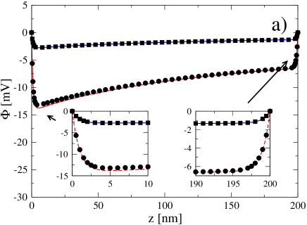
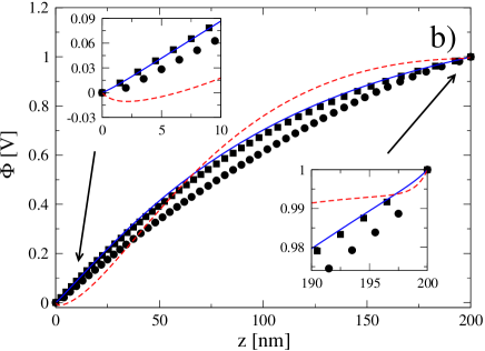
Figure 2: (Color online) Potential profile $\Phi(z)$ for $c_{\mathrm{L}}=c_{\mathrm{R}}=0.1$ M. Calculations are done for $\Phi(0)=\Phi(L)=0$ V (a) and $\Phi(0)=0$ V, $\Phi(L)=1$ V (b). Solid line and squares: $\sigma=-0.02$ e/nm², dashed line and circles: $\sigma=-0.1$ e/nm². Symbols in all cases stands for numerical solution, lines represent perturbation theory (first order in $\epsilon$). Insets depict closer look into left and right boundary layers.

It is clearly shown that the agreement with the analytical result (36), and (37) is getting worser with the increasing value of $\sigma$.

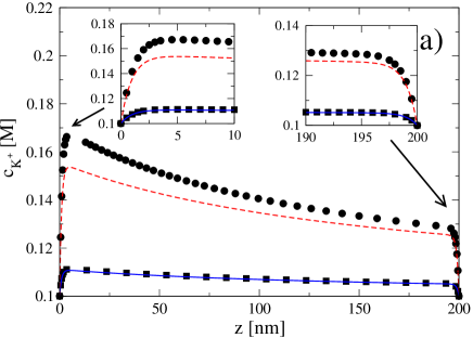
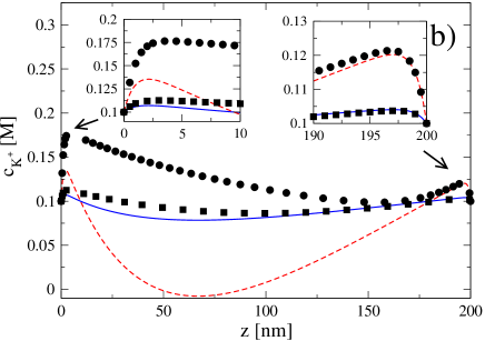
Figure 3: (Color online) Concentration profile $c_{\rm{K}^{+}}(z)$ for $c_{\mathrm{L}}=c_{\mathrm{R}}=0.1$ M. Calculations are done for $\Phi(0)=\Phi(L)=0$ V (a) and $\Phi(0)=0$ V, $\Phi(L)=1$ V (b). Solid line and squares: $\sigma=-0.02$ e/nm², dashed line and circles: $\sigma=-0.1$ e/nm². Symbols in all cases stands for numerical solution, lines represent perturbation theory (first order in $\epsilon$). Insets depict closer look into left and right boundary layers.

Moreover, the discrepancies between theory and numerics are more significant for growing absolute value of voltage. Figures 3-4 illustrate the situation in which the perturbation approximation starts to miscarry for the charge density $\sigma=-0.1$ e/nm² in the non-equillibrium situation when the transmembrane voltage reaches the value of 1 V. Note, in that case the perturbation theory also provides unphysical negative concentrations.

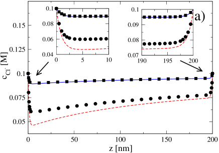
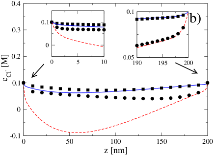
Figure 4: (Color online) Concentration profile $c_{\rm{Cl}^{-}}(z)$ for $c_{\mathrm{L}}=c_{\mathrm{R}}=0.1$ M. Calculations are done for $\Phi(0)=\Phi(L)=0$ V (a) and $\Phi(0)=0$ V, $\Phi(L)=1$ V (b). Solid line and squares: $\sigma=-0.02$ e/nm², dashed line and circles: $\sigma=-0.1$ e/nm². Symbols in all cases stands for numerical solution, lines represent perturbation theory (first order in $\epsilon$). In sets depict closer look into left and right boundary layers.

However, to assess the accuracy of power series in $\epsilon$, we shall systematically compare the approximations including higher orders of this parameter with numerical solutions. Such a process for the uniformly valid solutions of singular perturbation theory (including boundary layer solutions) is possible only up to second order in $\epsilon$. Nevertheless, on the basis of Theorem 2, one can note that the outer expansions approximate well the solutions of the 1D-PNP problem with the Donnan boundary conditions. One can obtain these perturbative expansions for any order in $\epsilon$.

5.1.2 Outer approximation

In the non-equillibrium situation, we examine the electric potential profile for $\epsilon=0.6$ (Fig. 2b), and the concentration profile for $\epsilon=0.12$ (Fig. 3b). Both approximations (in the first order of $\epsilon$) seem to show not too large discrepancy from the numerical solution. However, if we plot the same expansion in Eq. (36) with only one more term in the perturbation series, we notice a considerable deviation from the numerical results one when the transmembrane voltage becomes sufficiently large: $U=+1$ V, or $U=-1$ V (Fig. 5). This confirms that for the charge density $\sigma=-0.1$ the perturbation method fails totally. However, for a smaller charge density $\sigma=-0.02$ the perturbation theory works as demonstrated in Fig. 6,

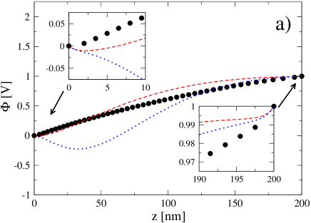
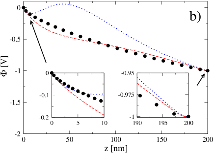
Figure 5: (Color online) Potential profile $\Phi(z)$ for $c^{\rm{Don}}_{\rm{K}^{+},~{}L}=156$ mM, $c^{\rm{Don}}_{\rm{K}^{+},~{}R}=125$ mM, $c^{\rm{Don}}_{\rm{Cl}^{-},~{}L}=87.3$ mM, $c^{\rm{Don}}_{\rm{Cl}^{-},~{}R}=83.6$ mM, $\sigma=-0.1$ e/nm². Calculations are done for $\Phi^{\rm{Don}}(0)=-0.014$ V, $\Phi^{\rm{Don}}(L)=0.994$ V (a) and $\Phi^{\rm{Don}}(0)=-0.014$ V, $\Phi^{\rm{Don}}(L)=-1.006$ V (b). We show perturbation solution in first order (in $\epsilon$): dashed line and second order: dotted line. The numerical solution is represented by symbols. Insets depict closer look into left and right boundary layers.

where the perturbation expansion was calculated up to the fourth order in $\epsilon$. One can notice that the agreement with numerics is getting better with growing order of the perturbative expansion. Then, it yields very accurate approximations in all aspects: the potential and concentration profiles, the total flux, and the electric current as well.

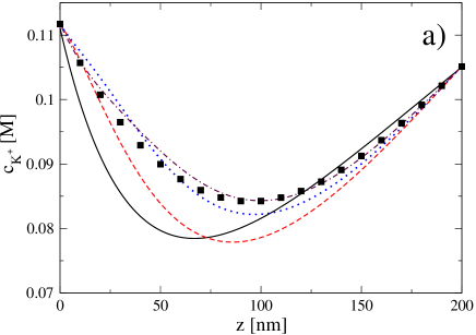
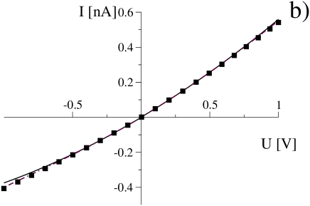
Figure 6: (Color online) In the upper panel (a) we show the concentration profile $c_{K^{+}}(z)$ for $\sigma=-0.02$ e/nm², and the Donnan b. c.: $c^{\rm{Don}}_{\rm{K}^{+},L}=112$ mM, $c^{\rm{Don}}_{\rm{K}^{+},R}=105$ mM, $c^{\rm{Don}}_{\rm{Cl}^{-},~{}L}=131.8$ mM, $c^{\rm{Don}}_{\rm{Cl}^{-},~{}R}=103.8$ mM, $\Phi^{\rm{Don}}(0)=-0.003$ V, $\Phi^{\rm{Don}}(L)=0.999$ V; and in the lower panel (b) we show the $I-U$ dependence. We show perturbation solution in first order (in $\epsilon$): solid line, second order: dashed line, third order: dotted line, and fourth order: dash-dotted line. The numerical solution is represented by symbols.

5.2 Rigorous b. c. vs. the Donnan b. c.

In Fig. 7, we compare the rigorous boundary layer solution with one given by the Donnan potential jump approximation. The both agree well except from the behavior in the boundary layer, where the ”Donnan” solution makes naturally a jump because it corresponds to the approximation of the boundary layer of zero-width. Note the agreement with the Theorem 2: the outer solutions agree very well.

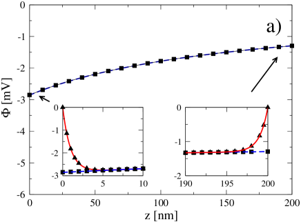
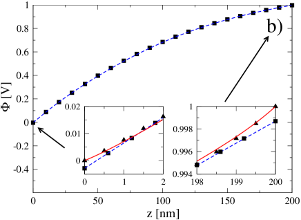
Figure 7: (Color online) Potential profile $\Phi(z)$ for $c_{L}=c_{R}=0.1$ M, $\sigma=-0.02$ e/nm². Calculations are done for $\Phi(0)=\Phi(L)=0$ V (solid line) and corresponding Donnan b. c. $\Phi^{\rm{Don}}(0)=-2.9$ mV, $\Phi^{\rm{Don}}(L)=-1.3$ mV (dashed line) (a); $\Phi(0)=0$ V, $\Phi(L)=1$ V (solid line) and corresponding Donnan b. c. $\Phi^{\rm{Don}}(0)=-0.003$ V, $\Phi^{\rm{Don}}(L)=0.999$ V (dashed line) (b). We show perturbation solution in first order (in $\epsilon$). Symbols in all cases stands for numerical solution, lines represent perturbation theory.

In Fig 8, we also compare the numerical solutions for the electric current in the case of the rigorous boundary conditions and in the case of the corresponding Donnan boundary condition approximation. The both solutions agree very well.

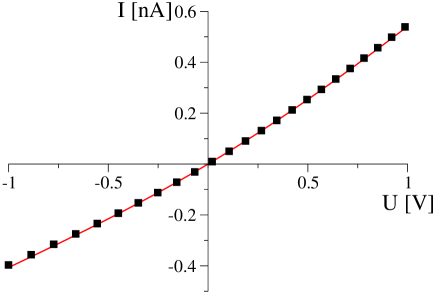
Figure 8: (Color online) Numerically obtained current voltage ($I-U$) characteristics for $\sigma=-0.02$ e/nm². Calculation are done for: rigorous b. c. (solid line) $c_{\mathrm{L}}=c_{\mathrm{R}}=0.1$ M and corresponding Donnan b. c. (squares) $c^{\rm{Don}}_{\rm{K^{+},L}}=112$ mM, $c^{\rm{Don}}_{\rm{K^{+},R}}=105$ mM, $c^{\rm{Don}}_{\rm{Cl^{-},~{}L}}=131.8$ mM, $c^{\rm{Don}}_{\rm{Cl^{-},~{}R}}=103.8$ mM.

6 Discussion

The studied 1D PNP model describes ion flows in the conical geometry in the presence of a permanent charge on the channel wall. The dimensionality reduction from 3D to 1D results both in an entropic potential asymmetry and in the appearence of an inhomogeneous, asymmetric 1D charge density. In this paper, we presented the details of the singular perturbation approach to the 1D PNP system including these profound effects. In another paper [4], these results are used further to find an analytical expression for the electric current and to quantify the rectification effect. When the surface charge density is small enough, the obtained theoretical expressions are expected to provide good approximations for the electric potential profile, concentrations of ions, the total flux, as well as for the electric current.

Although such weakly charged channels seem to be less interesting from the experimental point of view, they are important model systems [4]. In particular, based on our analytical solutions, complemented also by the numerical analysis, we studied and compared two different boundary conditions: the rigorous boundary conditions and the so-called Donnan boundary condition. The heuristic assumption of the Donnan equilibrium at the boundaries of the channel [8] in a highly non-equilibrium situation (current rectification) should and must be questioned. However, our analysis clearly showed that when the channel length exceeds much the Debye screening length, i.e. in the limit $1/\lambda\to 0$, the use of the Donnan boundary conditions is well justified.

Appendix A 1D model reduction

Let us start from the 3D electro-diffusion equation

$$\frac{\partial c_{i}(\vec{r},t)}{\partial t}=-\nabla\cdot\vec{j_{i}}(\vec{r},t)$$ (45)

where

$$\vec{j_{i}}(\vec{r},t)=-D_{i}\nabla c_{i}(\vec{r},t)+\rm{e}\nu_{i}\mu_{i}\vec{\mathcal{E}}(\vec{r})c_{i}(\vec{r},t)$$ (46)

defines the mass current $\vec{j_{i}}$ of the $i$-th species of ions, $\vec{r}$ is the position vector, $D_{i}$ is the diffusion constant, $\mu_{i}$ is the mobility of the ion particles, and $\vec{\mathcal{E}}(\vec{r})=-\nabla\Phi(\vec{r})$ denotes the electric field. The consistency with the thermal equilibrium demands that the mobility of the ions $\mu_{i}$ fulfills the Einstein relation, reading $D_{i}=\mu_{i}/\beta$, with the inverse temperature $\beta=1/k_{\rm{B}}T$.

The electric potential $\Phi({\vec{r}})$ is governed in a self-consistent manner by the Poisson equation

$$\epsilon_{0}\nabla\cdot[\epsilon({\vec{r}})\nabla\Phi({\vec{r}})]=-\sum_{i=\rm{K}^{+},\rm{Cl}^{-}}\rho_{i}({\vec{r}})-\rho_{\rm{fix}}({\vec{r}}),$$ (47)

where $\rho_{\rm{fix}}({\vec{r}})=\delta(r-R(z))\sigma$, with $\delta$ being the Dirac delta-function, represents the fixed charges located on the inside of the channel wall. $\rho_{i}({\vec{r}})$ denotes the density of mobile ions, and $\epsilon({\vec{r}})=\epsilon_{p}\Theta(r-R(z))+\epsilon_{w}\Theta(-r+R(z))$ describes dielectric properties of the system, with $\epsilon_{p},\epsilon_{w}$ being the relative dielectric constants of the polymer and water, respectively, and $\Theta$ being the Heaviside step function. In above-presented definitions we made use of cylindrical coordinates that are natural for the geometry given in Fig. 1.

The set of relations (45) and (47) for $\vec{j_{i}}=\rm{const}$ constitutes the system of coupled 3D Poisson-Nernst-Planck (PNP) equations.

Under assumptions of instantaneous equillibration in the transverse direction as in Eq. (3) and employing the definition of divergence given below (App. B) we derive the set of 1D PNP equations (Eqs. (5) and (6)), see also Ref. [4, 11].

Appendix B The divergence theorem.

The definition of the divergence of a vector $\vec{u}$ is

$$\nabla\cdot\vec{u}=\lim_{\mathcal{V}\to 0}\frac{1}{\mathcal{V}}\int_{\mathcal{S}}\vec{u}\cdot\hat{n}~{}dS=\lim_{\Delta z\to 0}\frac{1}{A(z)\Delta z}\int_{\mathcal{S}}\vec{u}\cdot\hat{n}~{}dS,$$ (48)

where $\mathcal{V}(z)=A(z)\Delta z$ denotes the volume surrounded by the closed surface $\mathcal{S}$ with the normal vector $\hat{n}$. For the flux field $\vec{j}(z)=j(z)\hat{e}_{z}$ (no ion flux across the channel wall) Eq. (48) can be reduced [12] to the form

$$\lim_{\Delta z\to 0}\frac{1}{A(z)\Delta z}\left[j(z+\Delta z)A(z+\Delta z)-j(z)A(z)]\right]=\frac{1}{A(z)}\frac{d}{dz}(A(z)j(z)).$$ (49)

In the case of the electric field we are intrested in the divergence: $\nabla\cdot\left(\epsilon(r,z)\vec{E}(z)\right)$. When $\vec{\mathcal{E}}(r,z)=\mathcal{E}_{z}(r,z)\hat{e}_{z}+\mathcal{E}_{r}(r,z)\hat{e}_{r}$ the surface $S$ is either parallel or perpendicular to $\vec{\mathcal{E}}$. Inside the channel the electric field has only the $z$ component depending on $z$ coordinate: $\vec{\mathcal{E}}(z)=\mathcal{E}_{z}(z)\hat{e}_{z}$. As the channel wall is charged with prescribed charge density $\sigma$, we find

$$\begin{array}[]{c}\displaystyle\vspace{10pt}\lim_{\Delta z\to 0}\frac{\epsilon_{w}}{A(z)\Delta z}\bigg{\{}\mathcal{E}(z+\Delta z)A(z+\Delta z)-\mathcal{E}(z)A(z)\bigg{\}}\\ \vspace{10pt}\displaystyle-\left(\epsilon_{p}\mathcal{E}^{\perp}_{\rm{polymer}}-\epsilon_{w}\mathcal{E}^{\perp}\right)\frac{2}{R(z)}\displaystyle=\frac{\epsilon_{w}}{A(z)}\frac{d}{dz}(A(z)\mathcal{E}(z))-\frac{2\sigma}{\epsilon_{0}R(z)},\end{array}$$ (50)

where $A(z)=\pi R^{2}(z)$. The jump in the electric field is due to the surface charge density (the electrostatic boundary condition on the channel wall):

$$\epsilon_{p}\mathcal{E}^{\perp}_{\rm{polymer}}-\epsilon_{w}\mathcal{E}^{\perp}=\frac{\sigma}{\epsilon_{0}}.$$ (51)

Appendix C The outer solutions - general expressions.

C.1 Zeroth order in $\epsilon$

In zeroth order in $\epsilon$, the solution reads

$$c^{(0)}_{(0),\mathrm{\Sigma}}(z)=\left(\frac{-J^{(0)}_{(0)}}{R(z)\gamma}+C^{(0)}_{(0)}\right)R^{2}(z).$$ (52)

Substituting that expression for the sum of concentrations in the second equation, we get

$$\Phi^{(0)}_{(0)}(z)=-I^{(0)}_{(0)}\int\frac{dz}{c^{(0)}_{(0),\mathrm{\Sigma}}(z)},$$ (53)

• $J^{(0)}_{(0)}=0$ if $c_{\mathrm{L}}=c_{\mathrm{R}}$ (see Appendix B)

  $$\Phi^{(0)}_{(0)}(z)=\frac{I_{(0)}^{(0)}}{C^{(0)}_{(0)}}\frac{1}{\gamma R(z)}+E^{(0)}_{(0)},$$ (54)

• $J^{(0)}_{(0)}\neq 0$ if $c_{\mathrm{L}}\neq c_{\mathrm{R}}$

  $$\Phi^{(0)}_{(0)}(z)=\frac{I_{(0)}^{(0)}}{J^{(0)}_{(0)}}\ln\frac{R(z)}{-J^{(0)}_{(0)}+C^{(0)}_{(0)}\gamma R(z)}+E^{(0)}_{(0)}.$$ (55)

C.2 First order in $\epsilon$

The solution reads

• $J^{(0)}_{(0)}=0$

  $$c^{(0)}_{(1),\mathrm{\Sigma}}(z) = \bigg{(}-\frac{\pi I^{(0)}_{(0)}}{C^{(0)}_{(0)}}\frac{1}{2\gamma R^{2}(z)}-\frac{J^{(0)}_{(1)}}{\gamma R(z)}+C^{(0)}_{(1)}\bigg{)}R^{2}(z)$$ (56)

• $J^{(0)}_{(0)}\neq 0$

  $$\begin{array}[]{c}\vspace{10pt}\displaystyle c^{(0)}_{(1),\mathrm{\Sigma}}(z)=\bigg{\{}\displaystyle\pi I^{(0)}_{(0)}\left(\frac{C^{(0)}_{(0)}\gamma}{J^{(0)~{}2}_{(0)}}\ln\left(\frac{-J^{(0)}_{(0)}+C^{(0)}_{(0)}\gamma R(z)}{R(z)}\right)+\frac{1}{J^{(0)}_{(0)}R(z)}\right)\\ \displaystyle-\frac{J^{(0)}_{(1)}}{\gamma R(z)}+C^{(0)}_{(1)}\bigg{\}}R^{2}(z).\end{array}$$ (57)

And the equation for the potential has the form

$$\Phi^{(0)}_{(1)}(z)=\int\frac{dz}{c^{(0)}_{(0),\mathrm{\Sigma}}(z)}\left\{-c^{(0)}_{(1),\mathrm{\Sigma}}(z)\frac{d\Phi^{(0)}_{(0)}(z)}{dz}-I^{(0)}_{(1)}+\pi R^{\prime}(z)\right\}.$$ (58)

C.3 Higher orders in $\epsilon$

The solution reads

$$\begin{array}[]{c}\vspace{10pt}\displaystyle c^{(0)}_{(2),\mathrm{\Sigma}}(z)=\vspace{10pt}\displaystyle\bigg{(}\mathcal{I}^{(0)}_{\{(0),(1)\}}(z)-\frac{J^{(0)}_{(2)}}{\gamma R(z)}+C^{(0)}_{(2)}\bigg{)}R^{2}(z),\end{array}$$ (59)

where $\mathcal{I}^{(0)}_{\{(0),(1)\}}$ denotes the part of solution that does not depend on coefficients of second order in $\epsilon$

$$\vspace{10pt}\displaystyle\mathcal{I}^{(0)}_{\{(0),(1)\}}(z) = \int dz\frac{c^{(0)}_{(1),\mathrm{\Sigma}}(z)}{R^{2}(z)c^{(0)}_{(0),\mathrm{\Sigma}}(z)}\left(J^{(0)}_{(1)}-\frac{d}{dz}c^{(0)}_{(1),\mathrm{\Sigma}}(z)+2\frac{R^{\prime}(z)}{R(z)}c^{(0)}_{(1),\mathrm{\Sigma}}(z)\right)$$ (60)

$$+ \int dz\frac{\pi\left(I^{(0)}_{(1)}-\pi R^{\prime}(z)R(z)\right)}{R(z)c^{(0)}_{(0),\mathrm{\Sigma}}(z)}.$$

And the equation for the potential for $n\geq 2$ has the form

$$\Phi^{(0)}_{\mathrm{(n)}}(z)=\int\frac{dz}{c^{(0)}_{(0),\mathrm{\Sigma}}(z)}\left\{-\sum^{n-1}_{m=0}c^{(0)}_{\mathrm{(n-m)},\mathrm{\Sigma}}(z)\frac{d\Phi^{(0)}_{\mathrm{(m)}}(z)}{dz}-I^{(0)}_{\mathrm{(n)}}\right\}.$$ (61)

The general solution for sum of concentrations for $n\geq 3$ reads

$$\begin{array}[]{c}\vspace{10pt}\displaystyle c^{(0)}_{\mathrm{(n)},\mathrm{\Sigma}}(z)=\displaystyle\bigg{(}\mathcal{I}^{(0)}_{\{(0),(1),\dots,\mathrm{(n-1)}\}}(z)-\frac{J^{(0)}_{\mathrm{(n)}}}{\gamma R(z)}+C^{(0)}_{\mathrm{(n)}}\bigg{)}R^{2}(z),\end{array}$$ (62)

where

$$\mathcal{I}^{(0)}_{\{(0),(1),\dots,\mathrm{(n-1)}\}}(z)=\sum^{n-1}_{m=1}\int dz\frac{c^{(0)}_{\mathrm{(n-m)},\mathrm{\Sigma}}(z)}{c^{(0)}_{(0),\mathrm{\Sigma}}(z)R^{2}(z)}\mathcal{B}_{\mathrm{m}}(z)+\int dz\frac{\pi I^{(0)}_{\mathrm{(n-1)}}}{R(z)c^{(0)}_{(0),\mathrm{\Sigma}}(z)}$$ (63)

with

$$\mathcal{B}_{\mathrm{m}}(z)=J^{(0)}_{\mathrm{(m)}}-\frac{d}{dz}c^{(0)}_{\mathrm{(m)},\mathrm{\Sigma}}(z)+2\frac{R^{\prime}(z)}{R(z)}c^{(0)}_{\mathrm{(m)},\mathrm{\Sigma}}(z).$$ (64)

The solution is iteratively given in orders of $\epsilon$. Note that, the solution, which is valid in the interior of the channel (called the outer expansion), is not valid near the both endpoints of the interval. Thus we have to find a different representation for the solutions near $z=0$ and $z=1$. These are boundary layer representation, which we consider in the next section. The outer expansion contain unknown constants $J^{(0)}_{(i)},I^{(0)}_{(i)},C^{(0)}_{(i)},E^{(0)}_{(i)}$, where $i=0,1,2,\dots$, which are determined by the matching condition.

Appendix D The outer solutions - determination of constants.

We obtain analytical formulas for the constants. In zeroth order in $\epsilon$, in the cases when

• $c_{\mathrm{L}}=c_{\mathrm{R}}=c$:

  $$\begin{array}[]{cc}\vspace{10pt}\displaystyle J^{(0)}_{(0)}=0,&\displaystyle C^{(0)}_{(0)}=2\pi c,\\ \vspace{10pt}\displaystyle I^{(0)}_{(0)}=-C^{(0)}_{(0)}(1+\gamma)\Phi_{\mathrm{R}},&\displaystyle E^{(0)}_{(0)}=\frac{(1+\gamma)}{\gamma}\Phi_{\mathrm{R}}.\\ \vspace{10pt}\displaystyle J^{(0)}_{(1)}=\frac{1}{2}(\gamma+2)\pi\Phi_{\mathrm{R}},&\displaystyle C^{(0)}_{(1)}=\frac{\pi}{2\gamma}\Phi_{\mathrm{R}},\\ \displaystyle I^{(0)}_{(1)}=\frac{1}{12}\pi\gamma\Phi^{2}_{\mathrm{R}},&\displaystyle E^{(0)}_{(1)}=-\frac{(\gamma+2)}{24c\gamma^{2}}\Phi^{2}_{\mathrm{R}}.\end{array}$$ (65)

• $c_{\mathrm{L}}\neq c_{\mathrm{R}}$:

  $$\begin{array}[]{cc}\vspace{10pt}\displaystyle J^{(0)}_{(0)}=2\pi(1+\gamma)\left(c_{\mathrm{R}}-c_{\mathrm{L}}\right),&\displaystyle C^{(0)}_{(0)}=\frac{2\pi}{\gamma}\left(c_{\mathrm{R}}(1+\gamma)-c_{\mathrm{L}}\right),\\ \vspace{10pt}\displaystyle I^{(0)}_{(0)}=J^{(0)}_{(0)}\frac{\Phi_{\mathrm{R}}}{\ln\left(c_{\mathrm{L}}/c_{\mathrm{R}}\right)},&\displaystyle E^{(0)}_{(0)}=\frac{\ln(2\pi\gamma c_{\mathrm{L}})}{\ln(c_{\mathrm{L}}/c_{\mathrm{R}})}\Phi_{\mathrm{R}}.\end{array}$$ (66)

For higher orders these calculations get pretty quickly tedious. Moreover, the formulas are very long. Thus, we do not present them explicitly. Instead, we propose a simple algorithm that we implemented in Maple.

Algorithm:

• $c^{(0)}_{(0),\mathrm{\Sigma}}(z)$ (Eq. (52)) and $\Phi^{(0)}_{(0)}(z)$ (Eq. (53))

• $\displaystyle\mathcal{I}^{(0)}_{(0)}(z)=\pi I^{(0)}_{(0)}\int dz/\left(R(z)c^{(0)}_{(0),\mathrm{\Sigma}}(z)\right)$

• $\displaystyle J^{(0)}_{(1)}=(1+\gamma)\left(\mathcal{I}^{(0)}_{(0)}(0)-\mathcal{I}^{(0)}_{(0)}(1)\right)$

• $\displaystyle C^{(0)}_{(1)}=J^{(0)}_{(1)}/\gamma-\mathcal{I}^{(0)}_{(0)}(0)$

• $\displaystyle c^{(0)}_{(1),\mathrm{\Sigma}}(z)=\left(\mathcal{I}^{(0)}_{(0)}(z)-J^{(0)}_{(1)}/\left(\gamma R(z)\right)+C^{(0)}_{(1)}\right)R^{2}(z)$

• $\displaystyle\Phi^{(0)}_{(1)}(z)$ (Eq. (58))

• $\displaystyle I^{(0)}_{(1)}=\rm{solve}\left(\Phi^{(0)}_{(1)}(0)-\Phi^{(0)}_{(1)}(1)+\tilde{\phi}^{(0)}_{(1)}(-\infty)-\phi^{(0)}_{(1)}(\infty),I^{(0)}_{(1)}\right)$

• $\displaystyle E^{(0)}_{(1)}=\rm{solve}\left(\Phi^{(0)}_{(1)}(0)-\phi^{(0)}_{(1)}(\infty),E^{(0)}_{(1)}\right)$

• $\displaystyle\mathcal{I}^{(0)}_{\{(0),\dots,\mathrm{n-1}\}}(z)$

  - for $n=2$: Eq. (60)

  - for $n\geq 3$: Eqs. (63) and (64)

• $$\vspace{10pt}J^{(0)}_{\mathrm{(n)}} = (1+\gamma)\bigg{(}\displaystyle\mathcal{I}^{(0)}_{\{0,\dots,\mathrm{n-1}\}}(0)-\mathcal{I}^{(0)}_{\{0,\dots,\mathrm{n-1}\}}(1)$$

  $$+ \displaystyle\frac{2}{(1+\gamma)^{2}}\sqrt{\tilde{p}^{(0)}_{\mathrm{(n)}}(-\infty)\tilde{n}^{(0)}_{\mathrm{(n)}}(-\infty)}-2\sqrt{p^{(0)}_{\mathrm{(n)}}(\infty)n^{(0)}_{\mathrm{(n)}}(\infty)}\bigg{)}$$

• $\displaystyle C^{(0)}_{\mathrm{(n)}}=\frac{J^{(0)}_{\mathrm{(n)}}}{\gamma}-\mathcal{I}^{(0)}_{\{0,\dots,\mathrm{n-1}\}}(0)+2\sqrt{p^{(0)}_{\mathrm{(n)}}(\infty)n^{(0)}_{\mathrm{(n)}}(\infty)}$.

• $c^{(0)}_{\mathrm{(n)},\mathrm{\Sigma}}(z)$ (Eqs. (59) and (62)) and $\displaystyle\Phi^{(0)}_{\mathrm{(n)}}(z)$ (Eq. (61))

• $\displaystyle I^{(0)}_{\mathrm{(n)}}=\rm{solve}\left(\Phi^{(0)}_{\mathrm{(n)}}(0)-\Phi^{(0)}_{\mathrm{(n)}}(1)+\tilde{\phi}^{(0)}_{\mathrm{(n)}}(-\infty)-\phi^{(0)}_{\mathrm{(n)}}(\infty),I^{(0)}_{\mathrm{(n)}}\right)$

• $\displaystyle E^{(0)}_{\mathrm{(n)}}=\rm{solve}\left(\Phi^{(0)}_{\mathrm{(n)}}(0)-\phi^{(0)}_{\mathrm{(n)}}(\infty),E^{(0)}_{\mathrm{(n)}}\right)$

In order to find values of $\bigg{\{}p^{(0)}_{\mathrm{(n)}}(\infty)$, $n^{(0)}_{\mathrm{(n)}}(\infty)$, $\phi^{(0)}_{\mathrm{(n)}}(\infty)\bigg{\}}$ and $\bigg{\{}\tilde{p}^{(0)}_{\mathrm{(n)}}(-\infty)$, $\tilde{n}^{(0)}_{\mathrm{(n)}}(-\infty)$, $\tilde{\phi}^{(0)}_{\mathrm{(n)}}(-\infty)\bigg{\}}$ we make use of the series expansion of the Donnan equilibrium conditions (LABEL:Donnan) at $z_{\mathrm{L}}$ and $z_{\mathrm{R}}$, respectively (see Theorem 1 in Sec. 4).

References

• [1] A. H. Nayfeh, Perturbation Methods (Pure and Applied Mathematics), (John Wiley and Sons, New York, 2000).
• [2] Z. Siwy, A. Apel, D. D. Dobrev, R. Neumann, R. Spohr, C. Trautmann, K. Voss, Nucl. Instr. Meth. B 208, 143 (2003).
• [3] Z. Siwy, Y. C. Gu, H. A. Spohr, D. Baur, A. Wolf-Reber, R. Spohr, P. Apel, Y. E. Korchev, Biophys. J. 82 266A, (2002); Z. Siwy, P. Apel, D. Baur, D. D. Dobrev, Y. E. Korchev, R. Neumann, R. Spohr, C. Trautmann, K.-O. Voss, Surf. Sci. 532-535, 1061 (2003). Z. Siwy, A. Fulinski Am. J. Phys. 72, 567 (2004).
• [4] I. D. Kosińska, I. Goychuk, M. Kostur, G. Schmid, and P. Hänggi, Phys. Rev. E 77, 031131 (2008).
• [5] M. B. Jackson, Molecular and Cellular Biophysics (Cambridge University Press, Cambridge, 2006).
• [6] R. A. Robinson and R. H. Stokes, Electrolyte Solutions, (Butterworth, London, 1955).
• [7] V. Barcilon, D.-P. Chen, R.S. Eisenberg, and J.W. Jerome, SIAM J. Appl. Math. 57, 631 (1997).
• [8] J. Cervera, B. Schied, R. Neumann, S. Mafe, and P. Ramirez, J. Chem. Phys. 124, 104706 (2006).
• [9] D. Gillespie, R. S. Eisenberg, Phys. Rev. E 63, 061902 (2001).
• [10] NAG Fortran Library Manual, Mark 20 (The Numerical Algorithm Group Limited, Oxford, England, 2001).
• [11] C. L. Gardner, W. Nonner, and R.S. Eisenberg, J. Comp. Electr. 3, 25 (2004).
• [12] G. Arfken, Mathematical Methods for Physicists (Academic Press, Orlando, FL, 1985).