Measuring Ages and Elemental Abundances from Unresolved Stellar Populations: Fe, Mg, C, N, and Ca

Abstract

We present a method for determining mean light-weighted ages and abundances of Fe, Mg, C, N, and Ca, from medium resolution spectroscopy of unresolved stellar populations. The method, pioneered by Schiavon (2007), is implemented in a publicly available code called EZ_Ages. The method and error estimation are described, and the results tested for accuracy and consistency, by application to integrated spectra of well-known Galactic globular and open clusters. Ages and abundances from integrated light analysis agree with studies of resolved stars to within $\pm 0.1$dex for most clusters, and to within $\pm 0.2$ dex for nearly all cases. The results are robust to the choice of Lick indices used in the fitting to within $\pm 0.1$ dex, except for a few systematic deviations which are clearly categorized. The realism of our error estimates is checked through comparison with detailed Monte Carlo simulations. Finally, we apply EZ_Ages to the sample of galaxies presented in Thomas et al. (2005) and compare our derived values of age, [Fe/H], and [$\alpha$/Fe] to their analysis. We find that [$\alpha$/Fe] is very consistent between the two analyses, that ages are consistent for old ($Age>10$ Gyr) populations, but show modest systematic differences at younger ages, and that [Fe/H] is fairly consistent, with small systematic differences related to the age systematics. Overall, EZ_Ages provides accurate estimates of fundamental parameters from medium resolution spectra of unresolved stellar populations in the old and intermediate-age regime, for the first time allowing quantitative estimates of the abundances of C, N, and Ca in these unresolved systems.

1 Introduction

The study of stellar populations in galaxies is going through very exciting transformations. The advent of extensive and high-quality data sets for galaxies in the local and distant universe poses a demand for ever improving stellar population synthesis models. In this paper, we present a new tool, named EZ_Ages, that simultaneously address two on-going needs in the field of stellar population synthesis: 1) it extracts accurate ages and abundances of several elements from integrated spectra of stellar populations, and 2) it performs this task in an automatic fashion, which is well-suited for applications to large data sets.

Early stellar population synthesis models for single-burst populations—so called “single stellar populations” or SSPs—were based on low resolution stellar spectra. The models of Worthey et al. (1994) and Vazdekis et al. (1996) used optical absorption-line indices with 8–10 Å resolution and limited spectral coverage, while Bruzual & Charlot (1993) synthesized model spectra with broad wavelength coverage (ultraviolet through infrared) and resolution of 10–20 Å in the optical. All models were for solar-abundance ratios only. Since then, a new generation of SSP models have pushed to higher resolution (2–3 Å for Bruzual & Charlot 2003 and Vakdekis et al. 2003) and to variable abundance patterns (Borges et al. 1995; Weiss et al. 1995; Tantalo et al. 1998; Trager et al. 2000; Thomas, Maraston, & Bender 2003; Maraston 2005; Schiavon 2007 and Coelho et al. 2007).

It is well known that many stellar populations, including the Galactic halo and bulge, Galactic globular clusters, massive early-type galaxies, and the bulges of spiral galaxies, have super-solar [$\alpha$/Fe]. In resolved systems, where abundance analysis of individual stars is possible, it has been known for a while that not all $\alpha$ elements are equally enhanced. On the other hand, in unresolved systems it has been only recently that evidence started accumulating to the fact that observed stellar populations have abundance patterns which cannot be described by only two parameters (ie. [Fe/H] and [$\alpha$/Fe]) but rather require more complicated abundance patterns. In particular, it seems that not all the $\alpha$ elements are equally enhanced in early-type galaxies (e.g., Vazdekis et al. 1997; Worthey 1998; Trager et al. 1998; Henry & Worthey 1999; Thomas, Maraston, & Bender 2003; Schiavon 2007). In the best studied, closest, resolved spheroidal system, the Galactic bulge, there is also recent evidence that not all $\alpha$-elements are equally enhanced (Fulbright, Rich, & McWilliam, 2005; Fulbright et al., 2007). In particular, Fulbright et al. (2007) found that, while Mg is strongly enhanced relative to Fe ([Mg/Fe] $\sim$ +0.3 across a range of [Fe/H]), other $\alpha$ elements such as Si, Ca, Ti, and O tend to follow a disk-like trend, with [X/Fe] decreasing with increasing [Fe/H]. Interestingly, in the case of oxygen—arguably the most important among the $\alpha$ elements—they found [O/Fe] $\approx 0$ at [Fe/H] = 0. Bensby, Feltzing, & Lundström (2004) show a similar result for Milky Way disk stars in both the thin and thick disk. Athey (2003) demonstrates that warm ionized gas in a sample of 7 local early-type galaxies has mean [O/H] $\approx-0.1$, while the stellar populations of the galaxies have super-solar [Mg/H]. Clues to variations of the abundances of other elements, such as C and N, particularly as a function of environment, have been found in a number of studies. The Lick indices C₂4668 and CN₂, which are sensitive to C and O (and N, in the case of CN₂), have been shown to be weaker in early-type galaxies in dense environments as compared to galaxies in the field, while the strength of the Mg b index remains unchanged across environments (Sánchez-Blázquez et al., 2003). Finally, a number of studies have found evidence that Ca seems to behave as an Fe-group element in elliptical galaxies, rather than following the trend of other $\alpha$ elements (Vazdekis et al. 1997; Worthey 1998; Trager et al. 1998; Henry & Worthey 1999; Thomas, Maraston, & Bender 2003). This result has recently been questioned by Prochaska et al. (2005) and Schiavon (2007), who show that the Ca4227 index is strongly affected by CN lines, which may be partially responsible for the low [Ca/Fe] suggested by other authors. Although $\alpha$-enhanced models are an important improvement over solar-scaled-only, it is fundamental that models with more degrees of freedom be developed, which are able to explore the complexity suggested by the data. By establishing a more detailed snapshot of the abundance patterns of stars in galaxies, these models can pose fundamental constraints on models of galaxy formation.

Schiavon (2007) presents a new set of SSP models which do exactly that. These models explicitly include adjustable abundance patterns for multiple elements, allowing the user to separately vary the abundances of C, N, O, Mg, Ca, Na, Si, Cr, and Ti. This paper describes an algorithm for searching through the space of variable abundance models to find the abundance mix which best fits the Lick indices measured in a given input stellar population spectrum. This algorithm has been implemented in an IDL code package, called “EZ_Ages” which is publicly available for use. Section 2 describes the sequential grid inversion algorithm. In §3, we present ages and abundances estimated by EZ_Ages for the Galactic globular clusters NGC 6121, 47 Tuc, NGC 6441, and NGC 6528, as well as the open cluster M67. These values are compared to results in the literature determined from isochrone fitting of cluster photometry and from high-resolution spectral abundance analysis for individual stars in the clusters. In §4 we apply EZ_Ages to galaxy data from the literature, contrasting our results with those by other authors. Section 5 summarizes our conclusions.

The beta-version of EZ_Ages is available for download, along with instructions on installation and use.

2 Sequential Grid Inversion Algorithm

2.1 Schiavon Simple Stellar Population Models

The code EZ_Ages is designed for use with the single stellar population models described in Schiavon (2007, hereafter S07). The details of the model are described in S07; here we briefly discuss the aspects of the model relevant to its practical use.

These models include a choice of two sets of isochrones by the Padova group: one is the solar-scaled isochrones of Girardi et al. (2000) and the other is the $\alpha$-enhanced set of isochrones by Salasnich et al. (2000) with average [$\alpha/$Fe$]=+0.42$ and with individual abundance ratios chosen to match metal-poor field stars. However, the models based on the $\alpha$-enhanced isochrone must be used with caution because Weiss et al. (2006) have shown that, due to a problem with the opacity tables adopted, those isochrones predict temperatures that are slightly too high at both the main-sequence turnoff and the giant branch. The effect is strongest at solar metallicity, where it results in ages that are slightly too old. For details, see §4.3 of S07. Developing isochrones with variable abundance ratios is an active area of current research (see recent work by Dotter et al. 2007) and we hope to incorporate a broader range of isochrones into EZ_Ages in the near future.

In addition to a choice of isochrones, the S07 models allow the user to select an input abundance pattern. The abundance ratios that can be varied are: [Mg/Fe], [C/Fe], [N/Fe], [O/Fe], [Ca/Fe], [Na/Fe], [Si/Fe], [Cr/Fe], and [Ti/Fe]. The S07 models output predicted Lick index measurements for a grid of age and [Fe/H] values, based upon the input abundance ratios. The models span the age range $0.1\leq t\leq 15.8$ Gyr, with $-1.3\leq$ [Fe/H] $\leq+0.2$ for the solar-scaled isochrone and $-0.8\leq$ [Fe/H] $\leq+0.3$ for the $\alpha$-enhanced isochrone, though only models older than 0.8 Gyr are computed with variable abundance ratios.

The Lick indices included in the S07 model are H$\delta_{A}$, H$\delta_{F}$, H$\gamma_{A}$, H$\gamma_{F}$, H$\beta$, CN₁, CN₂, Ca4227, G4300, Fe4383, C₂4668, Fe5015, Mg₂, Mg b, Fe5270, and Fe5335, as defined in Table 1 of Worthey et al. (1994) and Table 1 of Worthey & Ottaviani (1997). The output model indices can then be compared with Lick indices measured in the integrated spectrum of a real stellar population (i.e., a stellar cluster or a galaxy) to determine the best-fitting mean light-weighted age and [Fe/H] for the stellar population, for a given set of model abundance ratios.

The Lick indices included in the S07 model are summarized in Table 1, along with their main abundance sensitivities. These are taken from the works of Serven, Worthey, & Briley (2005) and Korn, Maraston, & Thomas (2005). The sensitivities from Korn, Maraston, & Thomas (2005) are taken from their Tables 4 and 5, which give abundance sensitivities for turnoff stars and giant branch stars respectively. We have chosen to include only those two evolutionary phases in the table, as they dominate the stellar population model spectrum (accounting for $\sim 90$% of the integrated light), even though all three evolutionary phases are taken into account in the model computations. In addition to the sensitivities to individual element abundances shown in the table, all indices are sensitive to changes in the total metallicity. We interpret the effect of [Z/H] on Fe5270 and Fe5335 as being due primarily to changes in Fe because none of the other elements investigated by KMT05 appear to affect these indices. Table 1 shows reasonable agreement between the two different sets of sensitivity tables.

Abundance variations enter the model in two ways, firstly through the choice of isochrone (solar-scaled or $\alpha$-enhanced). At this stage, the model takes into account the effect of the abundance mix on stellar evolution—specifically, how the chemical mix affects temperatures and luminosities of stars of different masses and at different evolutionary stages. Admittedly, this is done in an approximate fashion, given that unfortunately we only have isochrones computed for two abundance patterns. Secondly, the effect of individual elemental abundances on line and continuum opacities in stellar atmospheres is incorporated into model Lick index predictions, using the response functions computed by Korn, Maraston, & Thomas (2005). At this second stage, it is possible to vary elemental abundances independently; at the first stage, the only choices are [$\alpha$/Fe] = 0 and $+0.42$, with total metallicity varying.

It should be stated clearly that these models are cast in terms of [Fe/H], and not total metallicity, [Z/H]. This reflects our choice to deal explicitly with quantities that can be inferred from measurements taken in the integrated spectra of galaxies—total metallicity not being one of them, given our current inability to use integrated spectra of stellar populations to constrain the most abundant of all metals, oxygen (see discussion in §4.4.1 of S07). Another advantage with casting models in terms of [Fe/H] is that each elemental abundance can be treated separately, so that the effect of its variation can be studied in isolation from every other elemental abundance (at the cost of varying the total metallicity). In the case of models cast in terms of [Z/H], it is impossible to vary the abundance of a single element, because enhancing one element means decreasing the abundances of all other elements to keep total metallicity constant. As an example, in models cast in terms of [Z/H], a solar-metallicity ([Z/H] = 0) $\alpha$-enhanced population has only a slightly higher abundance of $\alpha$ elements than the Sun, while having a much lower iron-abundance. It is the large iron abundance difference that is responsible for the bulk of the difference between those two hypothetical models, not the small difference in $\alpha$-element abundances. For this reason, claims that higher order Balmer lines are strongly affected by $\alpha$-element abundances (Thomas et al., 2004) should be taken with caution (see §4.3 S07 for a thorough discussion of this point).

2.2 Fiducial Age and [Fe/H]

In practice, one would like to use absorption line measurements in the integrated spectrum of a given stellar population to determine not only the age and [Fe/H] for a fixed set of abundance ratios, but to find the best set of input abundances as well. The brute-force method of finding the best-fitting abundances would involve generating a set of models that span the available space of age, [Fe/H], and abundance patterns, and then identifying the model whose predicted Lick indices best match those measured in the spectrum. However, with nine variable abundance ratios, the search space quickly becomes very large. If each of those abundance ratios is represented by only four possible values, with 23 model ages and four possible values of [Fe/H], that would mean creating more than 24 million models!

Instead, we choose to perform a directed search for the best model, taking advantage of the fact that various Lick indices are sensitive to only a few, often different, elemental abundances, as indicated in Table 1. These sensitivity variations have been modeled by several groups using spectrum synthesis, based on model stellar atmospheres (see recent papers by Korn, Maraston, & Thomas 2005 and Serven, Worthey, & Briley 2005). A more detailed discussion of the motivation behind this method can be found in S07.

EZ_Ages begins by computing a set of models with the chosen isochrone (either solar-scaled or $\alpha$-enhanced), using solar abundance ratios for the stellar atmospheres. It then uses a pair of lines that are sensitive to age and [Fe/H], but relatively insensitive to other elemental abundances—a Balmer line and an Fe line—to determine a fiducial age and [Fe/H] for the stellar population in question. From Table 1 we can see that H$\beta$ and the iron lines Fe5270 and Fe5335 are good choices for determining the fiducial, as they are mostly insensitive to other element abundances. In EZ_Ages, the default choice of indices for calculating fiducial age and [Fe/H] are H$\beta$ and $\langle$Fe$\rangle$, an average of Fe5270 and Fe5335.

The top left panel of Figure 1 shows a plot of model grids for H$\beta$ and $\langle$Fe$\rangle$. Dotted lines connect constant-age models (from top to bottom: 1.2, 2.2, 3.5, 7.0, and 14.1 Gyr) while solid lines connect models with the same [Fe/H] (from left to right: -1.3, -0.7, -0.4, 0.0, and +0.2). The square shows a sample data point for a galaxy with age $\approx 7$ Gyrs and [Fe/H] $\approx-0.2$. In this figure, it is easy to see which box of the grid encloses the data point in question. This gives a bounded range in age and [Fe/H] for the data point. A two-dimensional linear interpolation within the gridbox is then used to convert the data point in index-index space into fiducial values for the age and [Fe/H].

2.3 Determining Non-Solar Abundance Ratios

Once a fiducial age and [Fe/H] have been determined from the H$\beta$–$\langle$Fe$\rangle$ model grid, one can then make a similar grid plot with an index which is sensitive to non-solar abundance ratios, for instance a Balmer line plotted against Mg b. Mg b is strongly affected by the [Mg/Fe] abundance ratio, at fixed [Fe/H]. If the chosen S07 model is a good match to the data, then the age and [Fe/H] estimated by grid inversion from the H$\beta$–Mg b plot should match the fiducial age and [Fe/H] from the H$\beta$–$\langle$Fe$\rangle$ plot. In our example in Figure 1, this is clearly not the case; the H$\beta$–Mg b plot in the top right panel of Figure 1 gives a larger value of [Fe/H] than the H$\beta$–$\langle$Fe$\rangle$ plot in the top left panel. This is an indication that the example galaxy has a larger [Mg/Fe] ratio than is predicted in a solar-scaled model. The sequential grid inversion algorithm then increases the input value of [Mg/Fe] and recomputes the S07 model. Increasing [Mg/Fe] will increase the strength of the Mg b index at fixed [Fe/H], which will have the effect of sliding the entire set of model grids to the right in the H$\beta$–Mg b plot, while keeping them essentially unchanged in the H$\beta$–$\langle$Fe$\rangle$ plane. This lowers the value of [Fe/H] that is estimated by grid inversion in the H$\beta$–Mg b plot, bringing it into agreement with that obtained in the H$\beta$–$\langle$Fe$\rangle$ diagram. This can been seen in the lower panels of Figure 1, which show H$\beta$–$\langle$Fe$\rangle$ and H$\beta$–Mg $b$ plots for an S07 model computed with [Mg/Fe]$=+0.3$. For the data shown in this plot, the age and [Fe/H] values indicated by the model grids are consistent for both metal lines. In the sequential grid-inversion algorithm implemented in EZ_Ages, [Mg/Fe] is increased incrementally until the [Fe/H] estimated from the H$\beta$–Mg b plot matches the fiducial [Fe/H] from the H$\beta$–$\langle$Fe$\rangle$ plot. This process is then repeated for other Lick indices and other abundance ratios.

The key to the sequential grid inversion algorithm is to proceed with the abundance fitting in such a way as to only adjust one abundance at a time. Once fiducial values for the age and [Fe/H] of the system have been determined, the goal is to next fit a Lick index that introduces only one additional abundance. Mg b is a good choice because it is dominated by Mg and Fe (see Table 1), with the latter being determined from the H$\beta$–$\langle$Fe$\rangle$ grid inversion. By adjusting [Mg/Fe] until the H$\beta$–Mg b grid inversion matches the fiducial values, EZ_Ages can find the best-fitting Mg abundance.

Another index which EZ_Ages can use to fit a single element is C₂4668, which is dominated by C and O. Oxygen is notoriously difficult to estimate in old (ie. non-star forming) unresolved stellar populations, therefore EZ_Ages does not try to model [O/Fe] (but see discussion in §3.2). Instead, it allows the user to choose an input oxygen abundance. For consistency, this should be chosen to match the input isochrone: [O/Fe] = 0.0 for the solar-scaled isochrone, [O/Fe] = +0.5 for the $\alpha$-enhanced isochrone. With [O/Fe] set by the user, this leaves only C as a variable abundance which contibutes strongly to C₂4668. EZ_Ages adjusts [C/Fe] so that the [Fe/H] estimated in the H$\beta$–C₂4668 plot matches the fiducial.

The only indices which are strongly affected by nitrogen and which might therefore allow a fit of [N/Fe] are the two CN lines, CN₁ and CN₂, both of which respond strongly to changes in C, N, and O. As discussed above, [O/Fe] is set by the user. This leaves C and N as variable abundances contributing to the CN indices. However, if [C/Fe] has already been determined by fitting C₂4668, then the CN indices can be used to fit for [N/Fe] at the calculated value of [C/Fe]. The computed value of [N/Fe] is therefore dependent upon the calculated value of [C/Fe] and a robust error analysis should propagate errors from [C/Fe] into the the errors in [N/Fe].

The S07 models include one Lick index dominated by Ca and can therefore be used to fit [Ca/Fe]: Ca4227. Because the blue continuum region used in measuring Ca4227 overlaps with a CN absorption band, this index is also very sensitive to [C/Fe] and [N/Fe], so that these abundance ratios must be fit properly before using Ca4227 to determine [Ca/Fe]. As with [N/Fe], errors in the calculated values of [C/Fe] and [N/Fe] contribute to the error in [Ca/Fe]. Again, this should be taken into consideration in a complete error analysis (see §2.4).

The set of available Lick indices and their element abundance sensitivities thus prescribe an order for abundance fitting: [C/Fe], then [N/Fe], then [Ca/Fe]. Note that Mg b, the preferred index used to fit [Mg/Fe], does not depend strongly on these abundances, nor do the other abundances depend on it, therefore it can be fit in any order.

Based on Table 1, it is clear that some indices are preferable for fitting: those that are dominated by the elemental abundances that we are using them to estimate and no others. Because of this, EZ_Ages has a built-in hierarchy which it uses to choose the indices used in abundance fitting. Among the Balmer lines, the preferred index is H$\beta$ because it is mildly sensitive to total metallicity, but relatively insensitive to individual abundances. It is followed by H$\delta_{F}$ and H$\gamma_{F}$, which are somewhat sensitive to individual elements, and lastly H$\delta_{A}$ and H$\gamma_{A}$, which are broader indices (designed to measure Balmer strengths in populations with a substantial A star component) and therefore include a larger number of other absorption features in the index and pseudo-continuum bandpasses.

For iron indices, the order of preference is $\langle$Fe$\rangle$ (an average of Fe5270 and Fe5335), Fe5270, Fe5335, Fe4383, and Fe5015. The indices Fe5270 and Fe5335 are dominated by Fe and total metallicity effects, making them relatively clean indicators of [Fe/H]. Of the other two lines, both of which are influenced by element abundance ratios, we prefer Fe4383 over Fe5015 for two reasons: Fe5015 falls on a CCD defect in the globular cluster data used in §3 to test the output of EZ_Ages and thus can only be tested for M 67, where it appears to perform similarly well to Fe4383, and the Fe5015 bandpass overlaps the [Oiii]$\lambda$5007 emission line from ionized gas sometimes present in galaxies, thus limiting its usefulness in stellar population modeling of galaxies.

For fitting [Mg/Fe], the preferred index is Mg b followed by Mg₂, which is more sensitive to C than is Mg b. For [C/Fe], it is C₂4668 followed by G4300, for reasons discussed in detail in §3.2. For [N/Fe], it is CN₁ followed by CN₂, although this is fairly arbitrary as there is no strong reason to prefer one CN index over the other. For [Ca/Fe], the only available index is Ca4227.

It is possible to manually override this order of preference if a given index is unavailable, or to investigate the effects of using other lines in the fit. Note that EZ_Ages will only fit an abundance ratio if at least one of the indices needed to estimate it is available. Also, abundances which depend on other abundance ratios will not be fit if the prerequisite abundance is not available (e.g., EZ_Ages will not use a CN index to fit [N/Fe] unless [C/Fe] has been determined from C₂4668 or G4300).

Thus far, we have focused only on the dominant abundances affecting each index, however many indices have a weak dependence on other abundances. Particularly if the most desirable Lick indices are not available due to limited wavelength coverage, bad skyline subtraction, or nebular emission within the galaxy and other lines have to be used (such as H$\delta_{F}$ in place of H$\beta$ or Fe4383 in place of Fe5270 or Fe5335), the computed fiducial values for age and [Fe/H] or other abundance values may change once the abundance fitting is complete, because some of the newly determined abundances may affect the indices used to determine those fiducial values. To ensure that the final abundance ratio is consistent for all of the Lick indices used in the fit, EZ_Ages iterates the fitting process up to four times. It uses the best-fitting abundance pattern from the previous iteration to compute new fiducial values for age and [Fe/H], then repeats the fitting process until further iterations do not improve the fit.

The S07 models account for variations in Lick index strength due to abundance variations in the elements Fe, Mg, C, N, Ca, O, Na, Si, Cr, and Ti. However, only the first five of these elements can be fit using the algorithm described above. The elements O, Na, Si, Cr, and Ti do not dominate any of the Lick indices modeled by S07 and therefore cannot be fit in this process. The EZ_Ages code allows the user to supply a value for any of these unmodeled elements to use as input to the S07 models. In the absence of user-supplied values, EZ_Ages has a set of default abundances for these elements. By default, it sets [O/Fe] to match the chosen isochrone ([O/Fe] = 0.0 for the solar-scaled isochrones, [O/Fe] = $+0.5$ for the $\alpha$-enhanced isochrone). The default for the $\alpha$-elements Na, Si, and Ti is that they are set to follow Mg, so that [Na/Fe] = [Si/Fe] = [Ti/Fe] = [Mg/Fe]. The iron-peak element Cr is set to follow Fe, so that [Cr/Fe] = 0.0. All of the modeling reported in this analysis was done using the default settings for the unmodeled elements and with the solar-scaled isochrone. To see the effect of using the $\alpha$-enhanced isochrone or super-solar [O/Fe] on abundance fitting, see §4.3 of S07 and Figures 12 and 14 in Graves et al. (2007).

2.4 Error Calculations

If errors in the Lick index data are provided as input, EZ_Ages uses them to estimate the uncertainties in the ages, [Fe/H], and abundance ratios calculated by the sequential grid inversion algorithm. Uncertainties are assumed to be dominated by measurement errors in the line strengths. Systematic uncertainties in the models are ignored, except that the usual caveat applies: comparisons of relative ages and abundances between multiple objects are more reliable than absolute age or abundance estimates.

Uncertainties in age and [Fe/H] due to line strength measurement errors are computed by displacing the measured data point by the input index error, then redoing the grid inversion on the displaced data point to determine the range in age or [Fe/H] constrained by 1$\sigma$ error in the measured Balmer or Fe line strength. Because the grid spacing is non-linear (particularly in age), errors in the positive and negative direction are computed separately. It has been noted by many previous authors that the errors in SSP age and [Fe/H] as inferred from index-index plots are not independent due to the fact that the model grids are not orthogonal. As can be seen from an inspection of Figure 1, age and [Fe/H] errors are correlated in the sense that lower inferred ages will lead to higher inferred [Fe/H], and vice versa. EZ_Ages does not explicitly model this aspect of the inferred errors in age and [Fe/H] values, but users should keep this effect in mind when interpreting results from SSP index-index fitting.

Any error in the choice of fiducial age and [Fe/H] will result in errors in the abundance ratios estimated by fitting to incorrect values of the age or [Fe/H]. Thus uncertainties in the fiducial age and [Fe/H] must be propagated through to determine their effect on the abundance ratio estimates.

For example, EZ_Ages assumes that the uncertainty in [Mg/Fe] is dominated by two sources: the measurement error of the Mg-sensitive Lick index used in the abundance ratio determination (e.g., Mg b) and the uncertainty in the fiducial [Fe/H] which EZ_Ages attempts to match in the H$\beta$–Mg b plot. In the following discussion, we will use $\Delta$Mg b and $\Delta$[Fe/H] to represent the measurement error in Mg b and the uncertainty in the fiducial [Fe/H], respectively. The uncertainty in [Mg/Fe] due to Mg b measurement error and fiducial uncertainty are denoted in turn by $\Delta$[Mg/Fe]_Mgb and $\Delta$[Mg/Fe]_fid.

To determine $\Delta$[Mg/Fe]_Mgb, EZ_Ages recomputes the [Mg/Fe] abundance for Mg b$+\Delta$Mg b and Mg b$-\Delta$Mg b, using the larger of these two uncertainties as the estimated $\Delta$[Mg/Fe]_Mgb. To determine $\Delta$[Mg/Fe]_fid, EZ_Ages recomputes [Mg/Fe] using the measured value of Mg b to fit [Fe/H]$+\Delta$[Fe/H] and [Fe/H]$-\Delta$[Fe/H], again choosing the larger uncertainty for estimating $\Delta$[Mg/Fe]_fid. These two sources of error are treated as independent and the total $\Delta$[Mg/Fe] is determined by summing in quadrature $\Delta$[Mg/Fe]_Mgb and $\Delta$[Mg/Fe]_fid.

The process for computing $\Delta$[C/Fe] is identical to that for [Mg/Fe], substituting a C-sensitive Lick index for Mg b. Because [N/Fe] is determined using a CN-sensitive index such as CN₁, $\Delta$[N/Fe] depends not only on the CN₁ line strength measurement error and $\Delta$[Fe/H], but on $\Delta$[C/Fe] as well. The contributions to $\Delta$[N/Fe] due to $\Delta$CN₁ and $\Delta$[Fe/H] (i.e., $\Delta$[N/Fe]_CN1 and $\Delta$[N/Fe]_fid) are computed as above. An additional contribution due to $\Delta$[C/Fe] is determined by matching the measured CN₁ line strength to the fiducial [Fe/H], using models with carbon abundances given by [C/Fe]$+\Delta$[C/Fe] and [C/Fe]$-\Delta$[C/Fe]. These three sources of error are summed in quadrature to obtain $\Delta$[N/Fe]. A similar process is repeated for [Ca/Fe], with the sole difference that errors in [N/Fe] also contribute to the [Ca/Fe] error budget.

To check that this analysis provides a reasonable estimate of the actual statistical errors, we have used a Monte Carlo method to generate a large set of artificial “repeat measurements” of the Lick indices for a test stellar population and compared the resulting distribution of ages, abundances, and abundance ratios to the errors calculated by EZ_Ages. For our test data, we used Lick index values measured in a stack of $\sim$10,000 red sequence galaxy spectra taken from the Sloan Digital Sky Survey. As modeled by EZ_Ages, these correspond to a stellar population with a mean light-weighted age of 9.1 Gyr, with [Fe/H]$=-0.15$, [Mg/Fe]$=+0.17$, [C/Fe]$=+0.17$, [N/Fe]$=+0.07$, and [Ca/Fe]$=0.00$.

We ran four Monte Carlo simulations for different error ranges (effectively different $S/N$ spectra), in which we assumed the errors were 2%, 5%, 10%, and 20% of the measured index values. For each run, we simulated 100 repeat measurements of the data by choosing values for each Lick index drawn from Gaussian distributions centered on the “true” data values with widths characterised by the assumed 2%, 5%, 10%, and 20% errors. This produced a simulation of 100 realizations for each of the four assumed error ranges. EZ_Ages was used to determine the age, [Fe/H], and abundance ratios for each simulated measurement. The distribution of these values for the 100 simulated repeat measurements can be compared with the error estimate made by EZ_Ages for the original data values and index measurement errors.

This comparison is shown in Figure 2. The errors reported by EZ_Ages are shown on the x-axis, while the y-axis shows the standard deviation $\sigma$ of the distributions of ages and abundances produced in each Monte Carlo simulation. As discussed earlier in this section, EZ_Ages calculates separately errors in the positive and negative direction. There are thus two error values produced by EZ_Ages plotted against each Monte Carlo $\sigma$. The solid line shows a one-to-one relation. The dashed lines outline error estimates that are within $\pm 30$% of the 1$\sigma$ Monte Carlo spread.

For the simulations with 2%, 5%, and 10% index measurement errors, the age and abundance ratio error estimates from EZ_Ages are all within 30% of the results of the Monte Carlo simulation with the exception of the error in the H$\gamma_{F}$ age, which is overestimated by about 0.3 Gyr in the 2% error case. Although this is a substantial fraction of the simulated H$\gamma_{F}$ age error, it is well within the uncertainties in the modeling process, which are of order 1 Gyr in the $\sim 9$ Gyr age range corresponding to the test data point (Schiavon, 2007). In all other cases, the EZ_Ages error estimate is an excellent match to the 1$\sigma$ errors produced by the full Monte Carlo realization. For the simulations with 20% index measurement errors, EZ_Ages tends to slightly overestimate the errors as compared to the Monte Carlo simulation, but in all cases is still within 35% of the simulated error.

The good match shown in this test between the error estimates generated by EZ_Ages and those produced by a Monte Carlo simulation of the errors suggests that EZ_Ages does in fact do a reasonable job of estimating the errors in the age, [Fe/H], and abundance ratio values calculated. This includes the propagation of errors between various stages of the modeling process. As the data become noisier, EZ_Ages has a tendency to slightly overestimate the actual uncertainty in the age, [Fe/H], and abundance due to measurement errors. Figure 2 also demonstrates that in order to estimate ages, [Fe/H], and abundance ratios within $\pm$0.1 dex for a typical early type galaxy, Lick indices must be measured with $\pm 5$% accuracy, which requires spectra with $S/N\sim 100$ Å^-1 (Cardiel et al., 1998).

2.5 Correlation of Errors in Derived Parameters

The Monte Carlo error simulation also allows us to investigate the effect of correlated errors in the EZ_Ages analysis. Because lines of constant age and [Fe/H] are not orthogonal in H$\beta$-$\langle$Fe$\rangle$ space, errors in either index measurement will result in anti-correlated errors in the inferred age and [Fe/H], as discussed in detail in Trager et al. (2000). For example, an error in H$\beta$ that causes the determined SSP age to be too old will cause the measured [Fe/H] value to be too low, as can be seen from the grids in Figure 1. Likewise, the sequential grid inversion process for fitting abundance ratios depends on the fiducial age and particularly on the fiducial [Fe/H] determination. This will tend to produce an anti-correlation between [Fe/H] and the measured abundance ratios.

As shown in Figure 2, the simplified error propagation implemented in EZ_Ages does an excellent job of tracking the total error in each stellar population parameter throughout the fitting process. However, it does not produce a full error ellipse illustrating correlated errors.

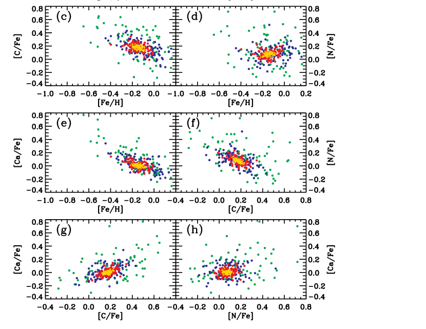
Figure 3: The distribution of EZ_Ages results for the Monte-Carlo error simulation. Yellow, red, blue, and green points correspond to the realizations of a single data point drawn from the 2%, 5%, 10%, and 20% error simulations, respectively. These trace out the error ellipses of the EZ_Ages fitting analysis and reveal the effect of correlated errors.

Figure 3 uses the results of the Monte Carlo error simulation to illustrate the correlated errors that result from sequential abundance fitting. The 100 simulated data realizations for each of the assumed 2%, 5%, 10%, and 20% index measurement errors (yellow, red, blue, and green points, respectively) effectively trace out the error ellipses in stellar population parameter space. Figure 3a shows the well-known error anti-correlation between the age and [Fe/H] measurements, as expected from the non-orthogonality of the age and [Fe/H] model grids in H$\beta$-$\langle$Fe$\rangle$ space.

Panels b–e show the abundance ratio determinations for [Mg/Fe], [C/Fe], [N/Fe], and [Ca/Fe] against [Fe/H]. The error ellipses for these data are expected to show an anti-correlation of errors because an over-estimate of [Fe/H] will tend to result in an under-estimate of the other abundances. For example, if an error in the $\langle$Fe$\rangle$ index causes the fiducial [Fe/H] determination to be too high, the measured abundance ratios for other elements will tend to be too low (at a higher [Fe/H], a lower value of [Mg/Fe] is needed to match the same Mg $b$ index). This anti-correlation is observed between [Fe/H] and the abundances [Mg/Fe], [C/Fe], and [Ca/Fe]. Interestingly, there appears to be no correlation in the errors in [Fe/H] and [N/Fe]. Because [N/Fe] is fit using a CN index, it depends strongly on the value of [C/Fe] previously determined by fitting either C₂4668 or G4300 and thus we expect a anti-correlation of errors between [C/Fe] and [N/Fe]. This is indeed the case, as illustrated in Figure 3f, and may explain the lack of correlation in the errors in [N/Fe] and [Fe/H]. As in the case of [N/Fe], the fitted values of [Ca/Fe] depend on other abundance fits and thus may produce correlated errors. These are illustrated in Figure 3g,h.

The effect of correlated errors can produce spurious trends in a dataset, thus the correlations illustrated here should be kept in mind when interpreting abundance patterns from EZ_Ages or a similar abundance fitting process. Of course, the best guard against these effects is to perform abundance fitting only on spectra with $S/N\geq 100$ Å^-1, corresponding to 5% index errors (red points in Figure 3) or better.

3 Testing the Models on Cluster Spectra

The validation of stellar population synthesis models depends crucially on their ability to match the integrated properties of simple systems, such as stellar clusters, which can be reasonably approximated by single stellar populations. In fact, this simple truism disguises the considerable complexity of the task, as attested by the vast literature dedicated to using cluster observations to constrain stellar population synthesis models (S07; Lee & Worthey 2005; Proctor et al. 2004; Schiavon et al. 2004a, b; Maraston et al. 2003; Schiavon et al. 2002a, b; Beasley et al. 2002; Vazdekis et al. 2001; Gibson et al. 1999; Schiavon & Barbuy 1999; Bruzual et al. 1997; Rose 1994; and references therein). S07 presented a lengthy discussion of the comparison of his models with integrated data for well-known Galactic open and globular clusters. Models were computed for a range of ages and metallicities, adopting the known abundance patterns of M 5, 47 Tuc, NGC 6528, and M 67. These were then compared with Lick index measurements taken in the (very high S/N) cluster spectra. As a result, it was found that predictions for Balmer and metal lines agreed with the data to within 1-$\sigma$ index measurement errors. Also very importantly, the best-matching ages differed by no more than $\sim$1 Gyr from the value obtained from analysis of cluster color-magnitude diagrams (CMDs). The only exception was M 5, for which the age found was too low, due to the presence of blue horizontal branch (HB) stars, which are not accounted for by the models (see §3.2 for a further discussion of this point).

In this section we ask the inverse question: how well do the models fare when used to convert a given set of index measurements into ages and elemental abundances? Again, we rely on data for clusters whose abundances and ages are well constrained from analysis of individual stellar spectra and deep cluster CMDs. Two important model checks are performed. We start by submitting the models to the most challenging of the two tests (§3.1), which consists of checking whether the results obtained with EZ_Ages match those from detailed resolved analysis of high-resolution spectra and deep photometry of stellar members. While our goal is to match ages and the abundances of Fe, Mg, C, N, and Ca to within 0.1 dex our requirement is that differences be smaller than 0.2 dex. Moreover, this set of specifications should be met in a quick and non-interactive fashion, suitable for applications to large data sets through use of EZ_Ages. As a second check (§3.2), we verify the internal consistency of EZ_Ages, by comparing the results obtained for a given set of observations, when using different combinations of Lick indices as age and metal-abundance indicators.

The clusters of choice for this exercise are selected on the basis of availability of good quality age and metal abundance determinations (Table Measuring Ages and Elemental Abundances from Unresolved Stellar Populations: Fe, Mg, C, N, and Ca). They span a wide range of metallicities, from [Fe/H] $\sim$ –1.2 (NGC 6121) to nearly solar metallicity (M 67 and NGC 6528), and include both old and intermediate-age (M 67) clusters. Lick indices for these clusters are presented in Table 2.

3.1 Reality Check

In Figure 4 cluster data are compared with the S07 solar abundance pattern models in a few index-index plots to illustrate that solar-scaled models cannot match the full set of observed cluster indices. The indices displayed are the default age and metal-abundance indicators employed by EZ_Ages. S07 showed that H$\beta$, $\langle$Fe$\rangle$, Mg $b$, C₂4668, CN₁ (or CN₂), and Ca4227 are the most reliable, recommended indices for age, [Fe/H], [Mg/Fe], [C/Fe], [N/Fe], and [Ca/Fe] determinations. This will be explored further in §3.2. Henceforth, we will refer to this set of indices as the standard set.

The models displayed in Figure 4 were computed for the solar abundance pattern, and the data were measured in the integrated spectra of the above globular clusters from the Schiavon et al. (2005) spectral library and that of M 67, obtained by Schiavon et al. (2004a), and revised by S07. In the upper left panel, model and data are compared in the $\langle$Fe$\rangle$ vs. H$\beta$ plane. S07 showed that these indices are excellent indicators of [Fe/H] and age, respectively. While the $\langle$Fe$\rangle$ average index is relatively insensitive to the abundances of elements other than Fe, H$\beta$ is mostly sensitive to age, being only mildly sensitive to the overall metallicity of the stellar population. Therefore, the age and iron abundance of each cluster can be read fairly accurately from the position of the cluster data on the model grid—except for the case of NGC 6121 where the presence of blue HB stars affects the H$\beta$-based age (see discussion in §3.2). The remaining panels show plots of other metal-line indices against H$\beta$, and $\langle$Fe$\rangle$ against H$\delta_{F}$. In the metal-line vs. H$\beta$ plots, one can see that the positions on the model grids where the data for most clusters fall are different from those they occupy on the $\langle$Fe$\rangle$ vs. H$\beta$ plot. As discussed in §2.3, this is a clear indication that the abundance pattern of the cluster stars is different from that of the Sun. We apply the method presented in the previous section to determine the abundance pattern of the clusters.

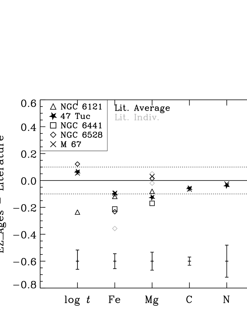
Figure 5: Comparison of EZ_Ages age ($\log t$), [Fe/H], [Mg/Fe], [C/Fe], [N/Fe], and [Ca/Fe] estimates with values from the literature. Error bars indicate the mean observational errors for our cluster data. Not all cluster parameters are available in the literature. For NGC 6528, two sets of abundances are available from different groups and these differe substantially (see Table Measuring Ages and Elemental Abundances from Unresolved Stellar Populations: Fe, Mg, C, N, and Ca). The individual literature values are plotted in gray, with an average of the two literature values plotted in black. For 47 Tuc, [C/Fe] and [N/Fe] abundances in the literature are computed separately for CN-weak and CN-strong stars. Here we compare the EZ_Ages results for [C/Fe] and [N/Fe] against the average over both sets of stars, as this best simulates their combined contribution to the integrated light

We ran EZ_Ages on the cluster data presented in Table 2. The results are listed in Table Measuring Ages and Elemental Abundances from Unresolved Stellar Populations: Fe, Mg, C, N, and Ca, together with abundance and age determinations from the literature. The literature values are based on abundance analyses of high-resolution spectra of individual cluster stars and on deep cluster CMDs, respectively. Differences between our results and those from the literature are displayed in Figure 5. In that plot, the dashed lines indicate the $\pm 0.1$ dex goal stated in the EZ_Ages specifications discussed in §3. Average values from the literature are displayed in black and individual determinations are shown in gray. For carbon and nitrogen, the values displayed are averages between CN-strong and CN-weak stars, as this best approximates the effect of unresolved spectroscopic observations.

A first inspection of the results shows that most abundance points fall between the two dashed lines, indicating that we are meeting the 0.1-dex goal for most of the abundances and for most clusters. Agreement is in fact particularly good for the abundances of carbon and nitrogen, where the 0.1-dex goal was reached for all clusters for which these elemental abundances are available in the literature. For magnesium and iron, we meet the 0.1-dex goal for some clusters, and the 0.2-dex requirement for all of them, with one exception: for NGC 6528, we find [Fe/H] = $-0.26$, in reasonably good agreement with the value [Fe/H] = $-0.15$ reported by Zoccali et al. (2004) and Barbuy et al. (2004) but in significant disagreement with the value [Fe/H] = $+0.1$ reported by Carretta et al. (2001). For calcium, there is one cluster only for which the 0.2-dex requirement is not met. For all the others, we meet the 0.1-dex goal. Given that this is the first systematic attempt at deriving abundances for all these five elements from integrated light, these results can be considered very satisfactory. Below we discuss the few exceptions for which agreement is not so good.

Although the values of [Fe/H] determined by EZ_Ages are almost all within the 0.2-dex requirement, they are consistently slightly lower than the literature abundances determined from invidual stars. The zeropoint for [Fe/H] in the models is based upon the [Fe/H] measurements for the stellar library from which the S07 model is constructed (the S07 models have not been separately calibrated to the Solar spectrum) and the zeropoint is not known to perfect accuracy. A systematic 0.1-dex underprediction of [Fe/H] by the models is possible. However, this is not necessarily more uncertain than the zeropoints in the cluster abundance determinations from individual stars. In the case of NGC 6528, for which multiple literature sources are available, the abundance determinations in the literature show substantial scatter: 0.25 dex in [Fe/H], 0.07 dex in [Mg/Fe], and 0.63 in [Ca/Fe]. In this context, it is difficult to address zeropoint issues on the order of 0.1 dex by comparison with existing cluster data.

In general we note that, for some clusters, elemental abundances determined by different groups are in substantial disagreement, which makes the task of interpreting our results a little more complicated. That is especially the case of NGC 6528 mentioned above, for which iron abundances from two groups differ by $\sim$ 0.25 dex, and calcium abundances differ by more than 0.6 dex! While a definitive statement on our ability to match that cluster’s abundances with EZ_Ages awaits the solution of this discrepancy, we call attention to the fact that agreement with the average values is very good.

EZ_Ages also performs very well in age determinations. For all clusters, with the sole exception of NGC 6121, the 0.2-dex requirement is met, and for 47 Tuc and M 67, the 0.1-dex goal is also achieved. For NGC 6121, the age obtained is too young because of the contribution by blue HB stars which tend to boost the strength of Balmer lines in the spectra of old stellar populations, mimicking a younger age (see §3.2). The effect of blue HB stars on Balmer lines has been pointed out in previous studies (Freitas Pacheco & Barbuy 1995; Maraston & Thomas 2000; Schiavon et al. 2004b; Trager et al. 2005; Schiavon 2007) and it can potentially lead to age underestimates.

The cluster NGC 6441 also contains blue HB stars (Rich et al., 1997), but EZ_Ages determines a relatively old age for the cluster when using the H$\beta$ index in the modelling process, which seems to contradict this interpretation. Unfortunately, we could not find a CMD-based age for this cluster in the literature so we cannot make a statement about how the age result from EZ_Ages compares to an independent age estimate. However, when the bluer Balmer line H$\delta_{F}$ is used in the modelling of NGC 6441, EZ_Ages finds a younger age than that determined from H$\beta$, suggesting that the influence of the blue HB stars does show up in H$\delta_{F}$. As discussed by Schiavon et al. (2004b), the signature of blue HB stars is stronger at bluer wavelengths, so that they tend to impact age determinations based on H$\delta$ more strongly than those based on H$\beta$. This can be clearly seen in the bottom right panel of Figure 4, where both NGC 6121 and NGC 6441 look younger in the $\langle$Fe$\rangle$ vs. H$\delta_{F}$ plot than in that involving H$\beta$.

In NGC 6441, the blue HB stars are greatly outnumbered by red HB stars, unlike NGC 6121 in which the blue HB population is substantial. They therefore have only a modest influence at the wavelength of H$\beta$, but a larger influence at the bluer wavelength of H$\delta_{F}$, where the blue HB stars contribute a greater fraction of the total light (Schiavon et al., 2004b). We further discuss this point in §3.2.

Finally, we note that the values we found for the abundances of C, N, and Ca for NGC 6121 are suspiciously low. Unfortunately, we could not find literature values for C and N abundances to compare with our estimates. However, the numbers Table Measuring Ages and Elemental Abundances from Unresolved Stellar Populations: Fe, Mg, C, N, and Ca and Figure 5 show that our [Ca/Fe] estimate is too low by about 0.3 dex, which confirms our suspicions that there might be a problem with our procedure for [Fe/H] $\mathrel{\hbox{\raise 2.15277pt\hbox{$<$}\hbox to0.0pt{\hss\lower 2.15277pt\hbox{$\sim$}}}}-1.0$. While this clearly deserves further investigation, for the time being we strongly discourage users from applying EZ_Ages in the [Fe/H] $\mathrel{\hbox{\raise 2.15277pt\hbox{$<$}\hbox to0.0pt{\hss\lower 2.15277pt\hbox{$\sim$}}}}-1.0$ regime.

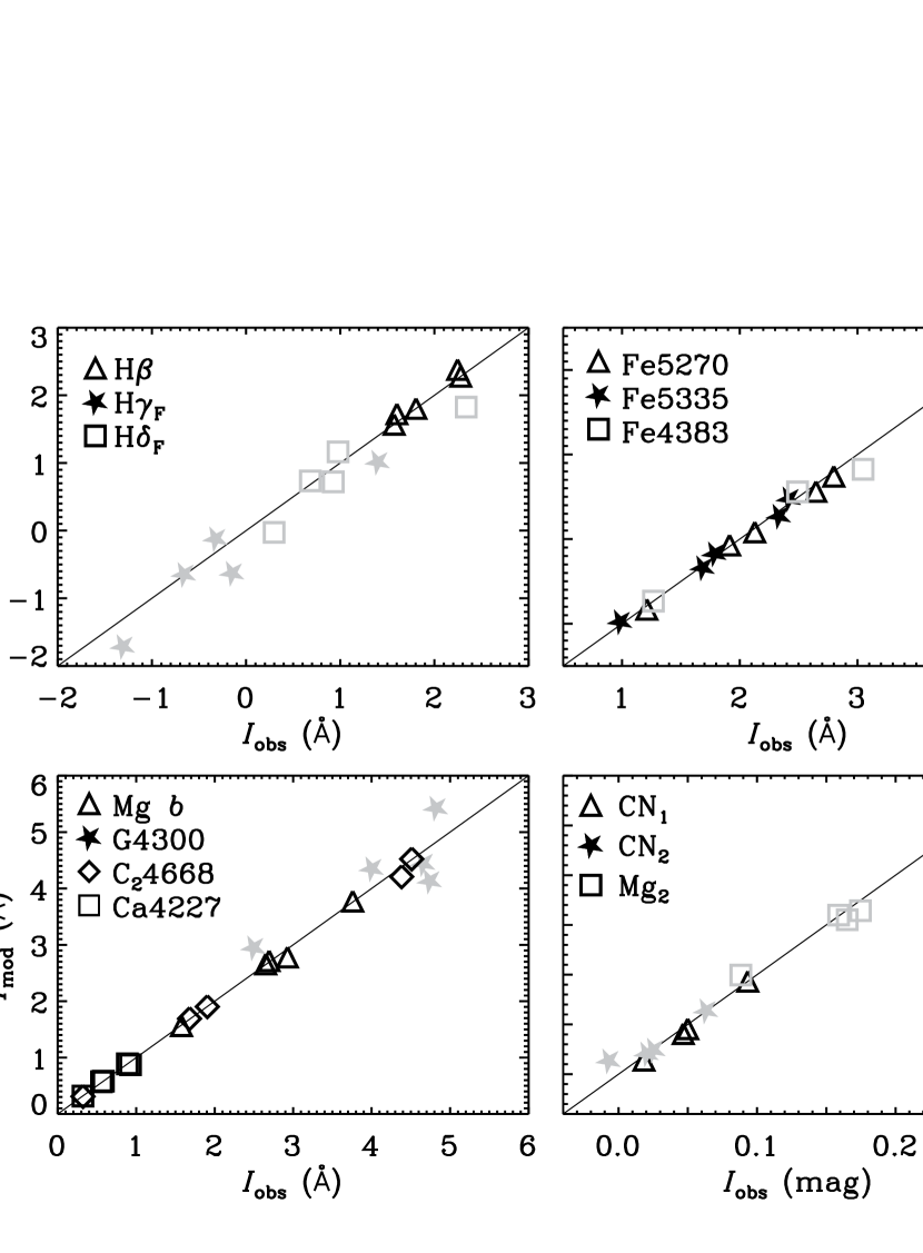
Figure 6: Comparison of observed Lick index measurements with the predicted index values from the best-fitting S07 model, as determined by EZ_Ages. All indices included in the S07 models are shown for each of the five test clusters. Measurement errors in the observed indices are approximately the size of the plotting symbols. Indices shown in black are those used in the abundance fitting process; those in gray are not used in the fitting. Solid lines show the one-to-one relation. Indices not used in the fitting process show some discrepancies between model predictions and the observed values, but there is no evidence for systematic discrepancies in the modeling of any of the indices.

Another check on the accuracy of the stellar population modeling is to compare the index predictions of the best-fitting model to the observed line strengths. Figure 6 shows the observed values of the Lick indices as measured in the five test cluster spectra, plotted against the predicted index line strengths from the best-fitting S07 model, as determined by EZ_Ages. Black and gray symbols show indices that are and are not included in the fitting process, respectively. The indices used in the fitting process are extremely well reproduced by the best-fitting model. In addition, the indices that are not used in the fitting process are also reasonably well matched by the model predictions, with some scatter but with no indication of systematic problems in the modeling of individual indices.

3.2 Consistency Check

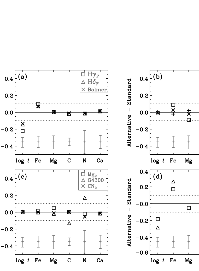
Figure 7: Variations in age ($\log t$), [Fe/H], [Mg/Fe], [C/Fe], [N/Fe], and [Ca/Fe] estimates for NGC 6441 from using different indices in the fitting process. Model names correspond to those in Table 4. Error bars indicate the observational errors calculated by EZ_Ages for NGC 6441 using the standard set of indices. (a–c) Results from substituting one alternative index into the standard index set (i.e., substituting G4300 for C₂4668 to fit [C/Fe]), and also for using averages of lines (i.e., an average of all Balmer lines instead of H$\beta$). All combinations of indices give results consistent within $\pm 0.1$ dex, with the exception of the bluer Balmer lines (panel a), which underpredict the cluster age, and G4300 (panel c, triangle), which underpredicts [C/Fe] by $-0.13$ dex relative to the fit using C₂4668. The underprediction of [C/Fe] results in an overprediction of [N/Fe], as expected from the correlated errors between [C/Fe] and [N/Fe] (see Figure 3). (d) Results for an average of all indices and for fitting when only indices blueward of 4400Å are available (simulating higher redshift observations). Fitting with Fe4383 and H$\delta_{F}$ instead of $\langle$Fe$\rangle$ and H$\beta$ (as in the simulated high redshift case) results in substantially younger ages and higher [Fe/H]. See text §3.2 for details.

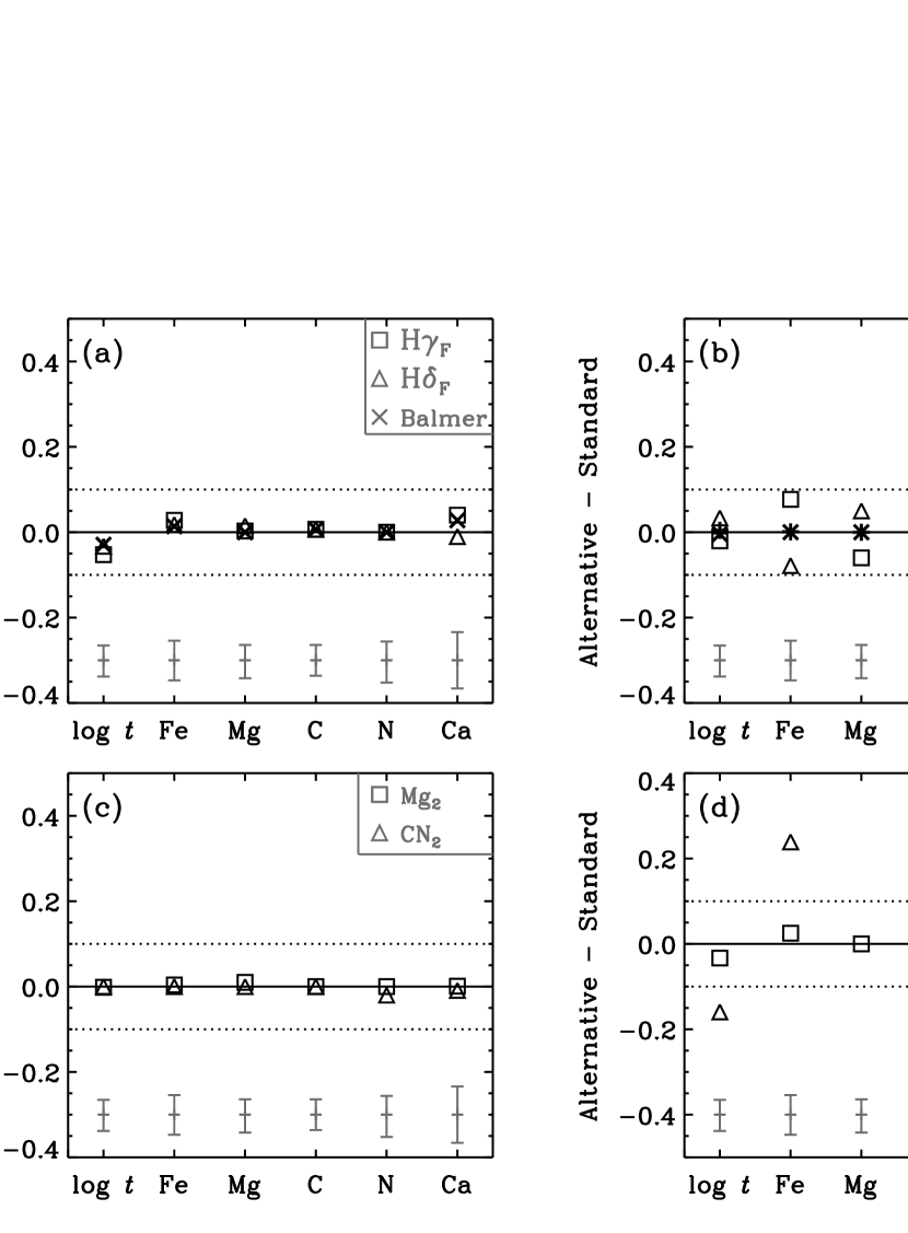
Figure 8: Variations in age ($\log t$), [Fe/H], [Mg/Fe], [C/Fe], [N/Fe], and [Ca/Fe] estimates for M 67 from using different indices in the fitting process. Model names correspond to those in Table 4. Error bars indicate the observational errors calculated by EZ_Ages for M 67 using the standard set of indices. (a–c) Results from substituting one alternative index into the standard index set (i.e., substituting G4300 for C₂4668 to fit [C/Fe]), and also for using averages of lines (i.e., an average of all Balmer lines instead of H$\beta$). (d) Results for an average of all indices and for fitting when only indices blueward of 4700Å are available (simulating higher redshift observations). Fitting with Fe4383 and H$\delta_{F}$ instead of $\langle$Fe$\rangle$ and H$\beta$ (as in the simulated high redshift case) results in substantially younger ages and higher [Fe/H]. See text §3.2 for details.

In this test, we verify how the results vary when different index sets are adopted as inputs to EZ_Ages. This is important, because the full set of indices considered by EZ_Ages are not always available to observers, due to limitations such as those determined by the instrumental setup adopted, or by the redshift of the sample studied. Therefore, it is important to make sure that age and metal abundances obtained from EZ_Ages do not depend on which absorption-line indices are employed—or, if they do, that the systematics is understood and can be accounted for. To test for this, we ran EZ_Ages on multiple combinations of line indices as measured for the clusters NGC 6441 and M 67, and inter-compared the ages and metal abundances obtained. As a basis for the comparisons, we adopt the results obtained when using the standard set, i.e., H$\beta$, $\langle$Fe$\rangle$, Mg $b$, C₂4668, CN₁, and Ca4227. The indices used in each separate model fit are listed in Table 4. We substitute each alternative index separately to asses the effect due to that individual index. We also examine some combinations of indices, specifically a “balmer” model, in which we fit using the average of H$\beta$, H$\gamma_{F}$, and H$\delta_{F}$, an “all” model, in which all lines are included in the fit, and a “high-z” model, which simulates the effect of applying EZ_Ages to higher redshift data, where only the bluer indices ($\lambda<4400$ Å) may be available because the indices at longer wavelengths are redshift out of the optical spectrum. Results from the fitting process are provided in Table 5 and displayed in Figures 7 and 8, where residuals relative to the age and metal abundances obtained with the standard index set are plotted for the various index combinations.

Looking first at NGC 6441, Figure 7 shows that, for the vast majority of the index combinations, ages and metal abundances vary by less than $\pm 0.1$ dex, indicating that EZ_Ages and the S07 models have attained an outstanding degree of consistency. There are a few exceptions, though, which occur for the following index combinations: 1) When G4300 is used as a carbon abundance indicator in place of C₂4668 (panel c, triangles); 2) When higher order Balmer lines are used as age indicators (panel a); 3) When higher order Balmer lines are used as age indicators and Fe4383 is used as the iron-abundance indicator as in the “high-z” model (panel d, triangles) or when the higher order Balmer lines and Fe4383 are averaged in with the other lines as in the “all” model (panel d, squares). In case 1, the G4300-based [C/Fe] and [N/Fe] values differ from those obtained from the standard indices by –0.14 and +0.18, respectively. In case 2, ages tend to be younger when higher-oder Balmer lines are used in place of H$\beta$, by up to $\sim$ –0.2 dex. Finally, case 3 is similar to case 2, except that [Fe/H] is too high, and consequently all the other abundances are too low.

The difference found in case 1 when replacing C₂4668 by the G4300 index is due to the different sensitivities of the two indices to the ratio between the abundances of carbon and oxygen (C/O). The two indices are sensitive to variations of the oxygen abundance because of details of the molecular dissociation equilibrium in the atmospheres of cool stars. Of all molecules in whose formation carbon and oxygen take part, carbon monoxide (CO) is the hardest one to break, because it has the highest dissociation energy. Therefore, at the temperatures prevalent in the atmospheres of G and K stars, most available free carbon and oxygen atoms are locked in CO. As a result, variations in the abundance of oxygen, usually the most abundant of the two species, have a strong influence on the amount of carbon that is free to form other molecules, such as C₂ and CH, which are responsible for the vibrational bands measured by the C₂4668 and G4300 indices, respectively. Therefore, an increase in the abundance of oxygen tends to provoke a decrease in the strength of those molecular bands.

While the concentration of the C₂ molecule depends quadratically on the abundance of carbon, that of CH depends only linearly on that abundance. As a result, C₂4668 is far more sensitive to carbon than to oxygen, while the the sensitivity of the G4300 index to those two abundances is approximately the same (though for both indices, the sensitivity to carbon and oxygen abundances have opposite signs). Although this makes the G4300 index a more uncertain indicator of carbon abundance, it raises the possibility that a combination of the two indices may be used to constrain the abundance of oxygen. We verified that possibility by raising the input oxygen abundance in the models from [O/Fe] = 0 to +0.3. As a result, the carbon and nitrogen abundances inferred from use of C₂4668 and G4300 indices agreed to within 0.05 dex. Furthermore, the ages and abundances inferred for the O-enhanced models were not substantially different from the results using the [O/Fe] = 0 model: [N/Fe] increased by $+0.12$ dex, while the ages inferred from H$\gamma_{F}$ and H$\delta_{F}$ increased by 0.6 Gyr. The values of H$\beta$ age, [Fe/H], [Mg/Fe], and [Ca/Fe] showed negligible change ($<0.1$ Gyr or $<0.05$ dex). Interestingly, the oxygen abundance in NGC 6441 stars ranges from [O/Fe] = –0.05 to 0.34 (Gratton et al., 2006), with stars in the upper end of the interval having “normal” oxygen abundances, and likely being more numerous and dominating the cluster light. Therefore, the value we obtained from the cluster’s integrated light is in good agreement with the known cluster abundance, which makes it possible that oxygen abundances might be inferred from a combination of the C₂4668 and G4300 indices. This will be further investigated in a forthcoming paper.

The dependence in case 2 of the resulting age on the Balmer line adopted is not surprising, given that NGC 6441 is characterized by the presence of blue HB stars (Rich et al. 1997, Busso et al. 2007). Because these stars have early-F and A spectral types, they tend to strengthen Balmer lines in the integrated spectra. That effect is obviously more important at bluer wavelengths, where the contribution by early-F and A stars to the integrated light is the greatest. Therefore, higher-order Balmer lines tend to be more strongly affected. As a result, when models that do not take into account blue HB stars are compared with the data, they tend to infer systematically younger ages, and more so according to higher order Balmer lines (see discussion in S07). Schiavon et al. (2004b) have in fact shown that this effect can be used to constrain the morphology of the HB of globular clusters, solely on the basis of Balmer line strengths in their integrated spectra. In particular, the ratio between H$\delta_{F}$ and H$\beta$ was shown to be very sensitive to the presence of blue HB stars.

Before discussing case 3, where Fe4383 and H$\delta_{F}$ are used in the fitting process, let us look at the results of the consistency test for M 67. Here again there is agreement to within $\pm 0.1$ dex for any combination of indices used, with the exception of combining Fe4383 and H$\delta_{F}$. The three Balmer lines all give consistent results for M 67 (panel a), because M 67 does not contain blue HB stars and because the integrated spectrum of M 67 used in the this analysis has been carefully constructed to exclude blue stragglers (Schiavon et al., 2004a). Unfortunately, there is a problem (as yet not well-understood) with the G4300 measurements for this cluster (Schiavon et al., 2004a), thus we cannot use M 67 to test our hypothesis about the effect of oxygen abundance on G4300 and C₂4668.

Indeed, the only inconsistency in the abundance determinations for M 67 is in the “high-z” model, in which Fe4383 and H$\delta_{F}$ are used in the fitting process (case 3 from above). Here, as with NGC 6441, we not only derive younger ages, but the resulting iron abundance is higher by $\sim+0.24$ dex. Consequently, all the other elemental abundances are found to be somewhat low. For M 67, we cannot invoke blue HB stars to explain this discrepancy. Interestingly, substituting H$\delta_{F}$ or Fe4383 into the standard index set individually (triangles in panel a and squares in panel b) does not result in large discrepancies from the standard model. How then can we understand the dramatic differences seen when both H$\delta_{F}$ and Fe4383 are used in the modelling process?

Figure 9 shows solar abundance model grids from the S07 model. The M 67 data are overplotted as diamonds. In panel a, we see that H$\beta$ and $\langle$Fe$\rangle$ produce model grids where lines of constant age and constant [Fe/H] are nearly perpendicular. This is one of the reasons this index combination is so useful for age and [Fe/H] determinations. When Fe4383 is substituted for $\langle$Fe$\rangle$ (panel b), the lines of constant [Fe/H] are less nearly vertical, lessening the diagnostic power of the index-index grid. Likewise, when H$\delta_{F}$ is substituted for H$\beta$ (panel c), the lines of constant age are less nearly horizontal, again constraining the age and [Fe/H] determinations. This is because, in the blue region, line crowding is higher, making H$\delta_{F}$ more sensitive to metallicity. Moreover, the blue spectral region is more strongly affected by warm stars than the red, making Fe4383 more sensitive to age than its redder counterparts. Notice, however, that there is still enough spread in the grids in panels b and c that small errors or zero-point uncertainties in the data or the models do not result in substatially different age and [Fe/H] measurements for M 67.

Now consider panel d. When H$\delta_{F}$ and Fe4383 are combined in the fitting process, the model grid lines are very far from perpendicular and the model space collapses down toward the familiar age-metallicity degeneracy. Here, small errors or zero-point uncertainties result in substantially different age and [Fe/H] measurements. Even the slight metallicity difference seen between panels a and b becomes a substantial discrepancy in panel d. This raises warning flags for using these indices to determine age and [Fe/H]. In particular, we note that Fe4383 appears to always give slightly higher values of [Fe/H] in the data presented both here and in ongoing work by the authors, suggesting that there is some inaccuracy in the modelling of this index. The fact that the discrepancy appears in the case of M 67, whose abundances are known to be solar-scale, suggests that this may be a zeropoint problem in the models, rather than a problem in calculating the abundance sensitivities of this index. Combined with the increased degeneracy of the H$\delta_{F}$-Fe4383 index-index space, this means that EZ_Ages should be used cautiously when determining stellar population parameters in higher redshift objects where H$\beta$ is not available, and that the need for high $S/N$ data is particularly acute in this regime. Even when the problem with Fe4383 is solved, the degeneracy of H$\delta_{F}$-Fe4383 index-index space means that small errors or zeropoint uncertainties in data can result in errors in the determination of age and [Fe/H] from these indices. This likely applies to all stellar population models, not just those presented in this work and S07.

In summary, we conclude that EZ_Ages is characterized by a remarkable degree of consistency, in that ages and metal abundances inferred from different index sets agree in the vast majority of cases to within $\pm 0.1$ dex. Two of the inconsistencies we found, namely, that different Balmer lines indicate different ages, and different carbon-abundance indicators indicate different carbon abundances, can in fact be potentially explored to extract even more information from the integrated spectra of stellar populations. While blue Balmer lines were shown to be useful to indicate the presence of blue HB stars in globular clusters (Schiavon et al., 2004b), the carbon index discrepancy can potentially be used to constrain the abundance of oxygen. The latter effect will be further investigated in a forthcoming paper. The third inconsistency is due to the fact that the combined H$\delta_{F}$-Fe4383 index-index space is substantially more degenerate than H$\beta$-$\langle$Fe$\rangle$ space, making accurate age and [Fe/H] determinations from these indices difficult. This is a matter of concern in integrated studies of globular clusters (Schiavon et al., 2004b) and higher redshift galaxies (Schiavon et al., 2006), for which only these bluer lines may be available.

4 Comparison with Abundance Modeling of Galaxies

Having performed the reality and consistency checks above, we now turn to comparisons between EZ_Ages results and those coming from application of other models in the literature. We focus on the models by Thomas, Maraston, & Bender (2003, hereafter TMB03), which also make predictions for variable abundance patterns. The TMB03 models also attempt to match non-solar abundance patterns by fitting Lick indices in unresolved stellar population spectra. These include both solar-scaled and $\alpha$-enhanced models, in which the set of $\alpha$ elements N, O, Mg, Ca, Na, Ne, S, Si, and Ti are slightly enhanced, while the iron peak elements Cr, Mn, Fe, Co, Ni, Cu, and Zn are significantly depressed, in order to vary [$\alpha$/Fe] at fixed total metallicity [Z/H]. In these models, [C/Fe] is fixed at solar.

Thomas et al. (2005, hereafter T05) use the TMB03 models to estimate ages, [Z/H], and [$\alpha$/Fe] for a sample of 124 early-type galaxies, based on measurement of the Lick indices H$\beta$, $\langle$Fe$\rangle$, and Mg $b$. To compare the stellar population modeling results of using EZ_Ages and the S07 models to those using TMB03, we have run EZ_Ages on the sample of 124 galaxies presented in T05, using the values of H$\beta$, $\langle$Fe$\rangle$, and Mg $b$ given in their Table 2. With these indices, EZ_Ages can determine the SSP age, [Fe/H], and [Mg/Fe] values of the sample galaxies and compare these results with those of the TMB03 models used in T05.

Although the details of the model fitting procedure differ, T05 perform a very similar analysis to that of EZ_Ages, determining age, [Z/H], and [$\alpha$/Fe] from the same Lick indices that are the standard set EZ_Ages uses to calculate age, [Fe/H], and [Mg/Fe]. The models used in T05 use the same Korn, Maraston, & Thomas (2005) index sensitivity functions as S07 and should therefore show the same index strength variations when the abundances are modified. One practical difference is that the TMB03 models are cast in terms of [Z/H], rather than [Fe/H]. In order to compare results from the two models, we convert T05’s estimated [Z/H] into [Fe/H] using the conversion proposed by TMB03: [Fe/H] = [Z/H] $-0.94$ [$\alpha$/Fe] (TMB03).

The TMB03 models assume that all $\alpha$-elements track Mg. EZ_Ages follows a similar convention, by default setting Na, Si, and Ti to track Mg in the modeling process, while Cr follows Fe. A significant advantage of EZ_Ages and the S07 models is that they also track the [C/Fe], [N/Fe], and [Ca/Fe] abundance ratios using C, N, and Ca-sensitive Lick indices, rather than making assumptions about how these elements vary. However, these differences should not affect the comparison of age, [Fe/H], and [$\alpha$/Fe] results presented here, as H$\beta$, $\langle$Fe$\rangle$, and Mg $b$ are predominantly sensitive to age, Fe and Mg only (see Table 1), and are thus treated the same by both models through the Korn, Maraston, & Thomas (2005) sensitivity functions.

The results of fitting the T05 galaxies using EZ_Ages are shown in Figure 10. In each panel, the dashed line shows a one-to-one relation and the solid line shows the best fitting line to the data while keeping the one-to-one slope fixed. The resulting zeropoint offsets between the model fits are indicated in the upper left corner of each panel. In general, there is good agreement between the results coming from application of the two models to the same data set. The scatter is small and the zeropoint offsets are modest. The values of [$\alpha$/Fe] agree to within a very small offset. The ages estimated in T05 are typically $\sim 25$% (0.13 dex) younger than those we find with EZ_Ages, while the T05 values of [Fe/H] are $\sim 0.08$ dex higher.

In addition to the zeropoint offsets in the age and [Fe/H] comparisons, the two different analyses do not truly follow a one-to-one slope for either parameter: the [Fe/H] relation is significantly steeper than the unity relation, while the age comparison shows some curvature. At old ages ($\log$ age $\mathrel{\hbox{\raise 2.15277pt\hbox{$>$}\hbox to0.0pt{\hss\lower 2.15277pt\hbox{$\sim$}}}}1.0$ as estimated by EZ_Ages) the slope is very nearly one-to-one, and the agreement between the two age estimates is much better, with a zeropoint offset of 15% ($-0.07$ dex) between the T05 ages and those from EZ_Ages. At intermediate ages ($0.8<\log\mbox{age}<1.0$ as estimated by EZ_Ages) the relation is steeper than unity, while at young ages ($\log\mbox{age}\mathrel{\hbox{\raise 2.15277pt\hbox{$<$}\hbox to0.0pt{\hss\lower 2.15277pt\hbox{$\sim$}}}}0.8$) the relation flattens out again, although at a substantial zeropoint offset. At intermediate and young ages, the T05 ages are 33% (0.17 dex in log age) younger. The origin of the curvature in the age relation is unclear. In any case, age agreement for old galaxies is very good (within 15%) and is still within 33% for all galaxies down to the youngest SSP ages estimated in the T05 sample.

Based on the cluster comparison of §3.1 and Figure 5, the zeropoint uncertainties in the S07 models are roughly 0.07 dex in $\log$ age, 0.1 dex in [Fe/H], and 0.05 dex in [Mg/Fe]. The differences between the T05 and the EZ_Ages results are therefore within the zeropoint uncertainties of the models, with the exception of the age estimates for galaxies younger than 10 Gyr. For these galaxies, the T05 results are younger by more than twice the indicated zeropoint uncertainties in the S07 and EZ_Ages models. The best way to resolve this discrepancy is to compare the models with data for metal-rich, intermediate-age clusters. While the models by S07 have been shown in the previous section and in Schiavon (2007) to match the data for M 67 ( $\sim$ 3.5 Gyr-old and solar metallicity), more data are clearly needed to better constrain the models in this crucial age/metallicity regime.

The non-unity slope of the [Fe/H] comparison also deserves further investigation. While the differences are negligibly small in the solar metallicity regime, they climb up to 0.2 dex at the high-metallicity end. For the most metal-rich galaxies, EZ_Ages obtains [Fe/H] $\sim$ 0.2, and T05 find galaxies to be more metal-rich by $\sim$ 0.2 dex. As in the case of age determinations, we again find ourselves lacking data that could help decide between the two model sets, given the non-existence of integrated spectroscopy for super-metal-rich clusters. It would be interesting, however, to compare results from the two models by confronting them with cluster data in a regime for which such data are available, such as moderately metal-poor clusters.

In Figure 11, we plot the difference between the values of [Fe/H] estimated in T05 and by EZ_Ages as a function of various other properties of the stellar populations . The top panel shows the [Fe/H] differences as a function of SSP age and $\alpha$-enhancement. The differences in the [Fe/H] estimates do not appear to be strongly correlated with either SSP age or $\alpha$-enhancement. In the lower panel, we show the differences in [Fe/H] as a function of the differences in the estimated ages and $\alpha$-enhancements. The [Fe/H] differences are correlated with differences in the age estimates between the two different models. Furthermore, the correlation is in the direction expected from the correlated errors in the index-index plots: where T05 obtain substantially younger ages than EZ_Ages, they also find higher [Fe/H]. The difference in the age estimates by the different models therefore naturally explains the observed differences in [Fe/H], both the zeropoint shift and the non-unity slope of the [Fe/H] comparison. Estimates of [$\alpha$/Fe] are substantially less biased by a zeropoint error in the age. That is because the Mg $b$ and $\langle$Fe$\rangle$ indices have very similar age-dependence, so that the zero-point uncertainties in the parameters determined by these two indices ([Mg/H] and [Fe/H]) cancel out.

From this analysis, it is clear that the TMB03 models and EZ_Ages give fairly consistent results, with a relatively small disagreement in the age zeropoints of the models which produces modest disagreements in [Fe/H]. Abundance ratios such as [$\alpha$/Fe] are much less sensitive to zeropoint offsets. The comparison of EZ_Ages results with ages from CMD fitting of Galactic clusters (§3) indicates that the age zeropoint in EZ_Ages is correct to within 0.07 dex in $\log$ age. The [Z/H] and [$\alpha$/Fe] results from TMB03 models have been compared with cluster data (Maraston et al., 2003; Thomas, Maraston, & Bender, 2003), but age estimates have not been independently tested, therefore it is difficult to say what the zeropoint uncertainties in the age determinations for these models should be. We therefore conclude that EZ_Ages and the S07 models give results in good agreement with the TMB03 models (at least in the high-metallicity regime tested in this analysis of galaxy spectra), but that at intermediate ages (age $<10$ Gyr) the TMB03 SSP ages may underestimate the true SSP ages by as much as 33% (0.17 dex in $\log$ age).

A more general result from this comparison is that the sequential grid inversion algorithm presented in this paper, combined with the SSP models of S07, does an excellent job of reproducing [Mg/Fe] abundances obtained by other groups with other models. Although the EZ_Ages abundance results for [C/Fe], [N/Fe], and [Ca/Fe] in unresolved stellar populations cannot be compared to other models (since no other models exist for the comparison), the modeling process for fitting these other abundances is the same as that used to fit [Mg/Fe] and the success of this process for [Mg/Fe] bodes well for other abundances. The test presented in this section, combined with the stringent tests with cluster data described in §3, are reassuring evidence that this modeling process is reasonable and can be used to provide a quantitative assessment of multiple elemental abundances.

5 Conclusions

In this paper, we have presented a methodology for measuring SSP ages, [Fe/H], and individual abundance ratios [Mg/Fe], [C/Fe], [N/Fe], and [Ca/Fe] for unresolved stellar populations. We do this by exploiting the different sensitivities of various Lick indices to a variety of elemental abundances, and the ability of the S07 stellar population models to accurately model the Lick indices for a wide range of input abundance patterns. The algorithm presented here has been implemented in the IDL code package EZ_Ages, which is available for download and general use.

We have subjected the modeling process described here to numerous rigorous tests and comparisons, with the following results:

• Comparison with Galactic cluster data:

  • Ages: EZ_Ages age estimates reproduce the results of cluster CMD fitting to within 0.15 dex for all clusters, with the exception of NGC 6121, whose Balmer line strengths are affected by a blue HB. For two out of three of the remaining clusters, the EZ_Ages age is within 0.1 dex of the CMD result.

  • [Fe/H] and [Mg/Fe]: EZ_Ages estimates match the results from high-resolution spectroscopy of individual cluster members to within 0.1 dex for some of the clusters, and to within 0.2 dex for all clusters (with the exception of the disagreement between our value of [Fe/H] for NGC 6528 and the results of Carretta et al. 2001—we are in $\sim\pm 0.1$ dex agreement with the results of Zoccali et al. 2004 and Barbuy et al. 2004 for [Fe/H] for this cluster).

  • [C/Fe] and [N/Fe]: For the only two clusters where C and N abundances are available (47 Tuc and M 67), EZ_Ages results match those from high-resolution spectroscopy of individual cluster members to within 0.1 dex. For NGC 6121, we find suspiciously low values, that might indicate a problem at the low metallicity end of our models. Therefore, we strongly caution users against using EZ_Ages to determine these abundances for systems with [Fe/H] $\mathrel{\hbox{\raise 2.15277pt\hbox{$<$}\hbox to0.0pt{\hss\lower 2.15277pt\hbox{$\sim$}}}}-1.0$.

  • [Ca/Fe]: EZ_Ages results are within $\sim 0.1$ dex for all clusters except NGC 6121. The latter is certainly related to the problem mentioned above regarding [C/Fe] and [N/Fe] in the metal-poor regime, so we do not recommend use of EZ_Ages for [Ca/Fe] determinations for systems with [Fe/H] $\mathrel{\hbox{\raise 2.15277pt\hbox{$<$}\hbox to0.0pt{\hss\lower 2.15277pt\hbox{$\sim$}}}}-1.0$.

• Consistency test performed on the cluster NGC 6441: using different combinations of Lick indices in the fitting process yields results that are consistent to within $\pm 0.1$ dex for all stellar population parameters except for the following cases:

  • Using G4300 instead of C₂4668 to fit [C/Fe] results in values of [C/Fe] and [N/Fe] that differ by $-0.14$ and $+0.18$ dex, respectively. This difference is probably due to differences in the index responses to O, which are not explored in this work.

  • Using H$\gamma_{F}$ or H$\delta_{F}$ instead of H$\beta$ as an age indicator results in younger ages for the cluster NGC 6441 due to the effect of the cluster’s blue HB. This discrepancy does not exist for M 67, which does not have a blue HB, and whose integrated spectrum is constructed to exclude blue HB stars.

  • Using the bluest Balmer and Fe lines available, H$\delta_{F}$ and Fe4383, can result in age and [Fe/H] measurements that are substantially different than those determined using the standard set of indices, due to the increased degeneracy of the model space for these indices. This poses a problem for high redshift studies of stellar populations, where often only the bluest lines are available for analysis.

• Error analysis test: EZ_Ages implements an algorithm that attempts to propagate errors through the modeling process in an efficient way that takes into account the dependence of abundance fitting on other parts of the population fitting process. Monte Carlo simulations show that this simplified error estimation does an excellent job of matching the true errors in the population parameters due to measurement errors in the Lick indices.

• Comparison with Thomas et al. (2005) results:

  • Results for [$\alpha$/Fe] are consistent between EZ_Ages results and those using TMB03 models.

  • Age and [Fe/H] comparisons show little scatter. There are zeropoint offsets of 15%–33% (0.07–0.17 dex) in age and 0.08 dex in [Fe/H] between the two analyses, and a non-unity slope in the [Fe/H] comparison. The age differences are small for the oldest (age $>10$ Gyr) galaxies and increase for younger galaxies. The [Fe/H] effects seem to be a natural result of the age differences. The S07 and EZ_Ages age zeropoints are shown here to be good to within 0.07 dex, while the TMB03 age zeropoints are untested. This suggests that the ages derived in T05 may be too young by up to 33% (0.17 dex) for intermediate age galaxies (age $<10$ Gyr).

  • Absolute estimates of abundance ratios are more reliable than absolute estimates of age or [Fe/H] because zeropoint uncertainties tend to cancel out.

  • The sequential grid inversion algorithm method is proven to work for estimating [Mg/Fe]. Since this method is the same as the one used to determine other abundance ratios, those estimates are likely to also be reliable, as demonstrated in the comparison with cluster data.

Overall, EZ_Ages and the S07 SSP models do an excellent job of fitting the SSP age, [Fe/H], and abundance ratios [Mg/Fe], [C/Fe], [N/Fe], and [Ca/Fe] for unresolved stellar populations. The small zeropoint uncertainties in age and [Fe/H] estimates illustrated by comparisons with Galactic cluster data demonstrate that absolute estimates can be made for these quantities with high $S/N$ data. Absolute estimates of elemental abundances are robust to the (small) zeropoint uncertainties. EZ_Ages and the S07 models therefore make it possible, for the first time, to perform a quantitative assessment of multiple individual elemental abundances from medium-resolution spectra of unresolved stellar populations. Furthermore, the abundance fitting process can be run in an automated way on large data sets. With these innovations, stellar population analysis is better positioned than ever before to address the task of unravelling the star formation histories of stellar systems.

Table 1: Lick Indices in the S07 SSP Models.

Index	KMT Sensitivity	SWB Sensitivity
Balmer Indices
H$\delta_{A}$	Fe, C-	Fe, C, V
H$\delta_{F}$	Fe, Mg+	Fe, C, Si
H$\gamma_{A}$	C, Fe, Mg	C, Ti, (Mg)
H$\gamma_{F}$	C, Fe	C, (Si), (Mg)
H$\beta$	…	(Ni)
Fe Indices
Fe4383	Fe, Mg, C-	C, Fe
Fe5015	Ti, Mg, Fe	C, Fe, (Ti)
Fe5270	Fe	C, (Fe)
Fe5335	Fe	Fe, C
Mg Indices
Mg2	Mg, C	Mg, C, Fe
Mg b	Mg, Fe, C	Mg, Fe, (Cr)
C, CH, and CN Indices
CN1	C, N, O	C, N, O
CN2	C, N, O	C, N, O
G4300	C, O, Fe+	C, Fe, Ti
C24668	C, O	C, O, (Si)
Ca Indices
Ca4227	Ca, C	Ca, O, (CN)

Note. — Index sensitivities as given by Korn, Maraston, & Thomas (2005, KMT) and Serven, Worthey, & Briley (2005, SWB). Only the top three element sensitivities are given, and only those with significance above 1$\sigma$ in the model spectra. For the KMT sensitivities, only those of turn-off and giant branch stars are shown, as these two components comprise 90% of the light in the S07 models. For the SWB sensivities, those under 2$\sigma$ are shown in parentheses.

Table 2: Selected Lick Indices for Clusters

	NGC 6121	47 Tuc	NGC 6441	NGC 6528	M 67	GC Err∗	M 67 Err
H$\delta_{F}$	2.338	0.682	0.926	0.298	0.977	0.117	0.090
H$\gamma_{F}$	1.398	-0.660	-0.148	-1.308	-0.324	0.215	0.050
H$\beta$	2.280	1.602	1.804	1.572	2.246	0.083	0.090
Fe4383	1.267	2.491	3.048	4.666	3.841	0.267	0.200
Fe5270	1.211	1.913	2.128	2.799	2.647	0.142	0.090
Fe5335	0.984	1.685	1.785	2.417	2.332	0.079	0.080
Mg b	1.577	2.694	2.651	3.759	2.927	0.148	0.100
Mg2	0.088	0.159	0.165	0.249	0.175	0.015	0.010
G4300	2.496	4.656	4.001	4.819	4.740	0.198	0.100
C24668	0.322	1.680	1.906	4.510	4.382	0.131	0.100
CN1	-0.070	0.025	0.020	0.063	-0.007	0.010	0.005
CN2	-0.047	0.050	0.047	0.093	0.018	0.008	0.008
Ca4227	0.321	0.557	0.581	0.887	0.927	0.041	0.100

Note. — All indices are measured in Å, except for CN₁ and CN₂, which are measured in magnitudes, as defined in Worthey et al. (1994).

Table 3: EZ_Ages Cluster Abundances Compared to Literature

		Age∗	[Fe/H]	[Mg/Fe]	[C/Fe]	[N/Fe]	[Ca/Fe]	Ref.
NGC 6121	EZ_Ages	$7.6_{-0.7}^{+0.8}$	$-1.30\pm 0.09$	$+0.36\pm 0.11$	$-0.12\pm 0.02$	$0.15\pm 0.15$	$-0.05\pm 0.10$
	literature	13‡	$-1.18\pm 0.00$	$+0.44\pm 0.02$	…	…	$+0.26\pm 0.02$	a, b
47 Tuc	EZ_Ages	$13.9_{-3.0}^{+\mbox{max\textdagger}}$	$-0.80\pm 0.09$	$+0.28\pm 0.05$	$-0.16\pm 0.03$	$+0.66\pm 0.08$	$+0.08\pm 0.03$
	literature	12	$-0.7\pm 0.05$	$+0.4\pm 0.1$	$-0.2$/$0.0^{**}$	$+1.1$/$+0.3^{**}$	$+0.2\pm 0.1$	c, d, e
NGC 6441	EZ_Ages	$11.5_{-1.5}^{+1.9}$	$-0.64\pm 0.07$	$+0.17\pm 0.08$	$-0.20\pm 0.05$	$+0.54\pm 0.13$	$+0.01\pm 0.08$
	literature	…	$-0.43\pm 0.08$	$+0.34\pm 0.09$	…	…	$+0.03\pm 0.04$	f, g
NGC 6528	EZ_Ages	$14.6_{-2.0}^{+\mbox{max\textdagger}}$	$-0.26\pm 0.06$	$+0.12\pm 0.06$	$-0.04\pm 0.04$	$+0.31\pm 0.08$	$-0.07\pm 0.05$
	literature	11	$-0.15$/$+0.1^{{\dagger}{\dagger}}$	$+0.07$/$+0.14^{{\dagger}{\dagger}}$	…	…	$-0.40$/$+0.23^{{\ddagger}}$	h, i, j, k
M 67	EZ_Ages	$4.0_{-0.58}^{+1.0}$	$-0.09\pm 0.05$	$0.03\pm 0.05$	$-0.07\pm 0.03$	$-0.01\pm 0.05$	$-0.03\pm 0.07$
	literature	3.5	$0.0\pm 0.1$	$0.0\pm 0.1$	$0.0\pm 0.1$	$0.0\pm 0.1$	$0.0\pm 0.1$	l, m, n

References. — (a) Salaris & Weiss 2002, (b) Ivans et al. 1999, (c) Schiavon et al. 2002a, b, (d) Briley et al. 2004, (e) Carretta et al. 2004, (f), (g) Gratton et al. (2006), (h) Ortolani et al. 2001, (i) Zoccali et al. 2004, (j) Barbuy et al. 2004, (k) Carretta et al. 2001, (l) Schiavon et al. 2004a, b, (m) Tautvaisiene et al. 2000, (n) Shetrone & Sanquist 2000

Table 4: Models Using Different Indices For Fitting

	Indices used in fit
Model name	Balmer	Fe	Mg	C	N	Ca
Standard	H$\beta$	$\langle$Fe$\rangle$	Mg b	C24668	CN1	Ca4227
H$\gamma_{F}$	H$\gamma_{F}$	$\langle$Fe$\rangle$	Mg b	C24668	CN1	Ca4227
H$\delta_{F}$	H$\delta_{F}$	$\langle$Fe$\rangle$	Mg b	C24668	CN1	Ca4227
Balmer	all	$\langle$Fe$\rangle$	Mg b	C24668	CN1	Ca4227
Fe4383	H$\beta$	Fe4383	Mg b	C24668	CN1	Ca4227
Fe5015	H$\beta$	Fe5015	Mg b	C24668	CN1	Ca4227
Fe5270	H$\beta$	Fe5270	Mg b	C24668	CN1	Ca4227
Fe5335	H$\beta$	Fe5335	Mg b	C24668	CN1	Ca4227
Mg2	H$\beta$	$\langle$Fe$\rangle$	Mg2	C24668	CN1	Ca4227
G4300	H$\beta$	$\langle$Fe$\rangle$	Mg b	G4300	CN1	Ca4227
CN2	H$\beta$	$\langle$Fe$\rangle$	Mg b	C24668	CN2	Ca4227
High-z	H$\delta_{F}$	Fe4383	…	G4300	CN1	Ca4227
All	all	all	all	all	all	Ca4227

Note. — For indices used in the fitting process, bold face indicates the index that differs from the standard set. “All” indicates that all available indices for that element were averaged together (i.e., fitting for [C/Fe] was done using an average of C₂4668 and G4300).

Table 5: EZ_Ages Results Using Different Indices For Fitting

	EZ_Ages results for NGC 6441							EZ_Ages results for M 67
Model	Age	[Fe/H]	[Mg/Fe]	[C/Fe]	[N/Fe]	[Ca/Fe]		Age	[Fe/H]	[Mg/Fe]	[C/Fe]	[N/Fe]	[Ca/Fe]
Standard	11.4	$-$0.64	$+$0.17	$-$0.20	$+$0.62	$+$0.04		4.0	$-0.09$	$+0.03$	$-0.07$	$-0.01$	$-0.03$
H$\gamma_{F}$	6.9	$-$0.54	$+$0.17	$-$0.22	$+$0.60	$+$0.05		3.5	$-0.07$	$+0.03$	$-0.06$	$-0.01$	$+0.01$
H$\delta_{F}$	8.2	$-$0.57	$+$0.17	$-$0.22	$+$0.60	$+$0.05		3.7	$-0.08$	$+0.05$	$-0.06$	$-0.01$	$-0.04$
Balmer	8.3	$-$0.57	$+$0.17	$-$0.21	$+$0.60	$+$0.05		3.7	$-0.08$	$+0.03$	$-0.06$	$-0.01$	$-0.01$
Fe4383	11.1	$-$0.55	$+$0.08	$-$0.25	$+$0.58	$-$0.04		3.8	$-0.02$	$-0.03$	$-0.10$	$-0.03$	$-0.09$
Fe5015†	…	…	…	…	…	…		4.3	$-0.17$	$+0.08$	$-0.02$	$-0.04$	$+0.01$
Fe5270	11.3	$-$0.62	$+$0.15	$-$0.21	$+$0.60	$+$0.01		3.9	$-0.10$	$+0.03$	$-0.07$	$-0.01$	$-0.03$
Fe5335	11.5	$-$0.66	$+$0.19	$-$0.19	$+$0.64	$+$0.06		4.0	$-0.09$	$+0.03$	$-0.07$	$-0.01$	$-0.03$
Mg2	11.4	$-$0.63	$+$0.22	$-$0.20	$+$0.60	$+$0.02		4.0	$-0.09$	$+0.04$	$-0.07$	$-0.01$	$-0.03$
G4300∗	11.6	$-$0.65	$+$0.15	$-$0.33	$+$0.79	$+$0.02		…	…	…	…	…	…
CN2	11.4	$-$0.64	$+$0.16	$-$0.20	$+$0.56	$+$0.02		4.0	$-0.09$	$+0.03$	$-0.07$	$-0.03$	$-0.04$
High-z∗	5.7	$-$0.34	$+$0.03	$-$0.33	$+$0.50	$-$0.10		2.7	$+0.15$	…	$-0.15$	$-0.04$	$-0.13$
All∗†	7.5	$-$0.47	$+$0.12	$-$0.26	$+$0.53	$-$0.02		3.7	$-0.07$	$+0.03$	$-0.06$	$-0.02$	$-0.01$

Figure 1: Grids produced by the S07 model illustrating the effects of super-solar [Mg/Fe]. Solid lines show constant [Fe/H] from left to right of -1.3, -0.7, -0.4, 0.0, and +0.2 ([Fe/H] = 0.0 is shown as a dashed line for reference). Dotted lines show constant age from top to bottom of 1.2, 2.2, 3.5, 7.0, and 14.1 Gyr. The square shows an example data point and is the same in both panels. Upper panel: Models computed with solar-scaled abundances. The Balmer-Fe grid gives fiducial values of $t=7$ Gyr and [Fe/H] = -0.2. The Balmer-Mg b grid shows an [Fe/H] $>0.4$ dex higher than the fiducial from the Balmer-Fe grid. This indicates that [Mg/Fe] is super-solar. Lower panel: Increasing [Mg/Fe] in the models slides the grid to the right toward the Balmer-Mg b data point, lowering the estimated [Fe/H]. H$\beta$ is also slightly affected by the abundance change, yielding a slightly younger fiducial age. In the Mg-enhanced model, the fiducial [Fe/H] from the Balmer-Fe grid matches the value of [Fe/H] estimated from the Balmer-Mg b grid, indicating that [Mg/Fe] $=+0.3$ is a good fit to the data.

Figure 2: Comparison of the error estimates determined by EZ_Ages with the results of the Monte Carlo error simulation. Age errors are plotted in the left panel and [Fe/H] and abundance errors in the right panel. The solid lines show one-to-one identity relations, with a $\pm 30$% spread indicated by dashed lines. The error estimates produced by EZ_Ages are consistent with those from the full Monte Carlo simulations, indicating that EZ_Ages produces reliable error estimates.

Figure 4: S07 solar-scaled model grids compared with cluster data. Model grids lines are as in Figure 1. Because H$\beta$ and $\langle$Fe$\rangle$ are relatively insensitive to non-solar abundance ratios, the fiducial age and [Fe/H] values for each cluster can be read off the model grid in the H$\beta$-$\langle$Fe$\rangle$ plot (upper left). If solar-scaled models were a good fit to all clusters, the data would fall in the same region of the model space in each index-index plot, as is approximately the case with M 67. The fact that other cluster data do not indicates that non-solar abundance patterns are needed to fit these clusters.

Figure 9: Solar abundance model grids showing the difficulty of measuring age and [Fe/H] from Fe4383 and H$\delta_{F}$. Lines of constant age run nearly horizontally and show (from top to bottom) 2.5, 2.8, 3.5, 5.0, 7.0, 8.9, and 14.1 Gyr models. Lines of constant [Fe/H] run nearly vertically and show (from left to right) $-0.4$, 0.0, and $+0.2$ dex models. The 3.5 Gyr and solar abundance model are shown with dashed lines for reference. Measured index values for M 67 are overplotted as the diamond. The standard indices (panel a) produce model grids with lines of constant age and constant [Fe/H] nearly perpendicular. Line of constant [Fe/H] are more sloped from the vertical when using Fe4383 instead of $\langle$Fe$\rangle$ (panel b). Similarly, lines of constant age are more sloped from the horizontal when using H$\delta_{F}$ instead of H$\beta$ (panel c). Substituting one or the other of these indices for the standard set causes only small offsets from the standard results (see Figure 8). However, the combination of Fe4383 and H$\delta_{F}$ (panel d) results in model grids that collapse down on one another, making the results much more sensitive to small errors or zeropoint uncertainties in either the models or the data. Because of the near-degeneracy of the models in Fe4383-H$\delta_{F}$ space, the combination of these two indices can give results substantially different from the age and [Fe/H] measured using the standard index set.

Figure 10: Comparison of $\log$ Age, [Fe/H], and [$\alpha$/Fe] results from T05 and from EZ_Ages. The galaxy sample is that of T05, and the stellar population parameters are from SSP fits to H$\beta$, $\langle$Fe$\rangle$, and Mg $b$ for each set of models. T05 models are cast in terms of [Z/H], which we compare to EZ_Ages values of [Fe/H] using the conversion given in TMB03 for their $\alpha$-enhanced mixture: [Fe/H] = [Z/H] - 0.94 [$\alpha$/Fe]. We compare their values of [$\alpha$/Fe] to the EZ_Ages results for [Mg/Fe], since T05 use the Mg $b$ line as their $\alpha$-enhancement indicator. Dashed lines show the one-to-one relation. Solid lines show the best fit one-to-one slope allowing for a zeropoint offset. The size and direction of the zeropoint offset are indicated in the top left of each panel. Error bars in the lower right corner of each panel indicate the median observational errors from T05. Results for [$\alpha$/Fe] are very consistent between the two models. T05 find ages which are younger by $\sim 35$% and [Fe/H] values which are higher by $\sim 0.08$ dex than the EZ_Ages results. Also, the slope of the [Fe/H] comparison differs somewhat from the one-to-one relation. These zeropoint differences, as well as the slope difference in [Fe/H], can be explained by differences in the model ages, which affect the [Fe/H] estimates, but have relatively little effect on [$\alpha$/Fe]. The age zeropoint difference between the models is somewhat larger than the zeropoint uncertainty in the S07 models (the age zeropoint of the models used in T05 is uncalibrated), suggesting that the T05 analysis may slightly underestimate the age of the sample galaxies. See text for details.

Figure 11: Top: Difference between [Fe/H] estimates for the T05 galaxy sample from EZ_Ages and from T05, as a function of stellar population age and [Mg/Fe]. Bottom: Difference in [Fe/H] as a function of differences in stellar population age and [$\alpha$/Fe]. The differences between T05 and EZ_Ages estimates of [Fe/H] are most strongly correlated with differences in the age results between the two models (lower left panel). This suggests that the non-unity slope of the [Fe/H] comparison relation in Figure 10 is due to differences in the age estimates and arises from correlated errors (see discussion in §2.4). The non-orthogonality of model grids in the index-index diagrams (as in Figure 1) results in correlated errors such that underestimating the age of a population will result in overestimating the corresponding value of [Fe/H].

References

- Athey (2003) Athey, A. E. 2003, PhD Thesis, University of Michigan
- Barbuy et al. (2004) Barbuy, B., et al. 2004, MmSAI, 75, 398
- Beasley et al. (2002) Beasley, M. A., Hoyle, F. & Sharples, R. M. 2002, MNRAS, 336, 168
- Bensby, Feltzing, & Lundström (2004) Bensby, T., Feltzing, S., & Lundström, I. 2004, A&A, 415, 155
- Borges et al. (1995) Borges, A.C., Idiart, T.P., de Freitas Pacheco, J.A. & Thevenin, F. 1995, AJ, 110, 2408
- Briley et al. (2004) Briley, M. M., Harbeck, D., Smith, G. H., & Gebel, E. K. 2004, AJ, 127, 1588
- Bruzual & Charlot (1993) Bruzual, G., & Charlot, S. 1993, ApJ, 405, 538
- Bruzual et al. (1997) Bruzual, G., Barbuy, B., Ortolani, S., Bica, E., Cuisinier, F., Lejeune, T., Schiavon, R.P. 1997, AJ, 114, 1531
- Bruzual & Charlot (2003) Bruzual, G., & Charlot, S. 2003, MNRAS, 344, 1000
- Busso et al. (2007) Busso, G., Cassisi, S., Piotto, G., Castellani, M., Romaniello, M., Catelan, M., Djorgovski, S.G., Recio Blanco, A., Renzini, A., Rich, M.R., Sweigart, A., & Zoccali, M. 2007, A&A, 105, 119
- Cardiel et al. (1998) Cardiel, N., Gorgas, J., Cenarro, J., & González, J. J. 1998, A&AS, 127, 597
- Carretta et al. (2001) Carretta, E., Cohen, J. G., Gratton, R. G., & Behr, B. 2001, AJ, 122, 1469
- Carretta et al. (2004) Carretta, E., Gratton, R. G., Bragaglia, A., Bonifacio, P., & Pasquini, L. 2004, A&A, 416, 925
- Coelho et al. (2007) Coelho, P., Bruzual, G., Charlot, S., Weiss, A., Barbuy, B., & Ferguson, J. W. 2007, MNRAS, 382, 498
- Dotter et al. (2007) Dotter, A., Chaboyer, B., Ferguson, J. W., Lee, H.-C., Worthey, G., Jevremović, D., & Baron, E. 2007, ApJ, 666, 403
- Freitas Pacheco & Barbuy (1995) Freitas Pacheco, J.A. & Barbuy B. 1995, A&A, 302, 718
- Fulbright, Rich, & McWilliam (2005) Fulbright, J. P., Rich, R. M., & McWilliam, A. 2005, Nuclear Physics A, 758, 197
- Fulbright et al. (2007) Fulbright, J. P., Rich, R. M.,& McWilliam, A. 2007, ApJ, 661, 1152
- Gibson et al. (1999) Gibson, B.K., Madgwick, D.S., Jones, L.A., Da Costa, G.S. & Norris, J.E. 1999, AJ, 118, 1268
- Girardi et al. (2000) Girardi, L., Bressan, A., Bertelli, G., & Chiosi, C. 2000, A&AS, 141, 371
- Gratton et al. (2006) Gratton, R. G., Lucatello, S., Bragaglia, A., Carretta, E., Momany, Y., Pancino, E., & Valenti, E. 2006, A&A, 455, 271
- Graves et al. (2007) Graves, G. J., Faber, S. M., Schiavon, R. P., & Yan, R. 2007, ApJ, submitted (astro-ph/0707.1523)
- Henry & Worthey (1999) Henry, R.B.C. & Worthey, G. 1999, PASP, 111, 919
- Ivans et al. (1999) Ivans, I. I., Sneden, C., Kraft, R. P., Suntzeff, N. B., Smith, V. V., Langer, G. E., & Fulbright, J. P. 1999, AJ, 118, 1273
- Korn, Maraston, & Thomas (2005) Korn, A. J., Maraston, C., & Thomas, D. 2005, /aap, 438, 685
- Lee & Worthey (2005) Lee, H.-c. & Worthey, G. 2005, ApJS, 160, 176
- Maraston (2005) Maraston, C. 2005, MNRAS, 362, 799
- Maraston & Thomas (2000) Maraston, C. & Thomas, D. 2000, ApJ541, 126
- Maraston et al. (2003) Maraston, C., Greggio, L., Renzini, A., Ortolani, S., Saglia, R.P., Puzia, T.H., & Kissler-Patig, M. 2003, A&A, 400, 823
- Ortolani et al. (2001) Ortolani, S., Barbuy, B., Bica, E., Renzini, A., Zoccali, M., Rich, R. M., & Cassisi, S. 2001, A&A, 376, 878
- Prochaska et al. (2005) Prochaska, L.C., Rose, J.A. & Schiavon, R.P. 2005, AJ, 130, 2666
- Proctor et al. (2004) Proctor, R.N., Forbes, D.A. & Beasley, M.A. 2004, MNRAS, 355 1327
- Rich et al. (1997) Rich, R.M., Sosin, C., Djorgovski, S.G., Piotto, G., King, I.R., Renzini, A., Phinney, E.S., Dorman, B., Liebert, J., & Meyla, G. 1997, ApJ, 484, L25
- Rose (1994) Rose, J.A. 1994, AJ, 107, 206
- Salaris & Weiss (2002) Salaris, M., & Weiss, A. 2002, A&A, 388, 492
- Salasnich et al. (2000) Salasnich, B., Girardi, L., Weiss, A., & Chiosi, C. 2000, A&A, 361, 1023
- Sánchez-Blázquez et al. (2003) Sánchez-Blázquez, P., Gorgas, J., Cardiel, N., Cenarro, J., & González, J. J. 2003, ApJ, 590, 91
- Schiavon (2007) Schiavon, R. P. 2007, ApJS, 171, 146
- Schiavon & Barbuy (1999) Schiavon, R.P. & Barbuy, B., 1999, ApJ, 510, 934
- Schiavon et al. (2002a) Schiavon, R. P., Faber, S. M., Castilho, B.V., & Rose, J. A. 2002a ApJ, 580, 850
- Schiavon et al. (2002b) Schiavon, R. P., Faber, S. M., Rose, J. A., & Castilho, B. V. 2002b, ApJ, 580, 873
- Schiavon et al. (2004a) Schiavon, R.P., Caldwell, N. & Rose, J.A. 2004a, AJ, 127, 1513
- Schiavon et al. (2004b) Schiavon, R.P., Rose, J.A., Courteau, S. & MacArthur, L. 2004b, ApJ, 608, L33
- Schiavon et al. (2005) Schiavon, R.P., Rose, J.A., Courteau, S. & MacArthur, L. 2005, ApJS, 160, 163
- Schiavon et al. (2006) Schiavon, R.P. et al. 2006, ApJ, 651, L93
- Serven, Worthey, & Briley (2005) Serven, J., Worthey, G., & Briley, M. M. 2005, ApJ, 627, 754
- Shetrone & Sanquist (2000) Shetrone, M. D., & Sanquist, E. L. 2000, AJ, 120, 1913
- Tantalo et al. (1998) Tantalo, R., Chiosi, C. & Bressan, A. 1998, A&A, 333, 419
- Tautvaisiene et al. (2000) Tautvaisiene, G., Edvardsson, B., Tuominen, I., & Ilyin, I. 2000, A&A, 360, 499
- Thomas, Maraston, & Bender (2003) Thomas, D., Maraston, C. & Bender, R., 2003, MNRAS, 343, 279
- Thomas et al. (2004) Thomas, D., Maraston, C. & Korn, A. 2004, MNRAS, 351, 19
- Thomas et al. (2005) Thomas, D., Maraston, C., Bender, R., & de Oliveira, C. M. 2005, ApJ, 621, 673
- Trager et al. (1998) Trager, S. C., Worthey, G., Faber, S. M., Burstein, D., & González, J. J. 1998, ApJS, 116, 1
- Trager et al. (2000) Trager, S. C., Faber, S. M., Worthey, G., & González, J. J. 2000, AJ, 120, 165
- Trager et al. (2005) Trager, S.C., Worthey, G., Faber, S.M. & Dressler, A. 2005, MNRAS, 362, 2
- Vazdekis et al. (1996) Vazdekis, A., Casuso, E., Peletier, R. F., & Beckman, J. E. 1996, ApJS, 106, 307
- Vazdekis et al. (1997) Vazdekis, A., Peletier, R.F., Beckman, J.E. & Casuso, E. 1997, ApJS, 111, 203
- Vazdekis et al. (2001) Vazdekis, A., Salaris, M., Arimoto, N. & Rose, J.A. 2001, ApJ, 549, 274
- Vakdekis et al. (2003) Vazdekis, A., Cenarro, A. J., Gorgas, J., Cardiel, N., & Peletier, R. F. 2003, MNRAS, 340, 1317
- Weiss et al. (1995) Weiss, A., Peletier, R.F. & Matteucci, F. 1995, A&A, 296, 73
- Weiss et al. (2006) Weiss, A., Salaris, M., Ferguson, J. W., & Alexander, D. R. 2006, astro-ph/0605666)
- Worthey (1998) Worthey, G. 1998, PASP, 110, 888
- Worthey, Faber, & González (1992) Worthey, G., Faber, S. M., & González, J. J. 1992, ApJ, 398, 69
- Worthey et al. (1994) Worthey, G., Faber, S. M., González, J. J., & Burstein, D. 1994, ApJS, 94, 687
- Worthey & Ottaviani (1997) Worthey, G. & Ottaviani, D. L. 1997, ApJS, 111, 377
- Zoccali et al. (2004) Zoccali, M., et al. 2004, A&A, 423, 507