The contribution of star formation and merging to stellar mass buildup in galaxies.

Abstract

We present a formalism to infer the presence of merging activity by comparing the observed time derivative of the galaxy stellar mass function (MF) to the change of the MF expected from the star formation rate (SFR) in galaxies as a function of galaxy mass and time. We present the SFR in the Fors Deep Field as a function of stellar mass and time spanning $9<\log M_{\ast}<12$ and $0<z<5$. We show that at $z\gtrsim 3$ the average SFR, $\dot{M}_{\ast}$, is a power law of stellar mass ($\dot{M}_{\ast}\propto M_{\ast}^{0.6}$). The average SFR in the most massive objects at this redshift are 100 – 500 $\mathrm{M_{\odot}}\mathrm{yr}^{-1}$. At $z\sim 3$, the SFR starts to drop at the high mass end. As redshift decreases further, the SFR drop at progressively lower masses (downsizing), dropping most rapidly for high mass ($\log M_{\ast}\gtrsim 11$) galaxies. The mass at which the SFR starts to deviate from the power-law form (break mass) progresses smoothly from $\log M_{\ast}^{1}\gtrsim 13$ at $z\sim 5$ to $\log M_{\ast}^{1}\sim 10.9$ at $z\sim 0.5$. The break mass is evolving with redshift according to $M_{\ast}^{1}(z)=2.7\times 10^{10}\,(1+z)^{2.1}$. We directly observe a relationship between star formation history (SFH) and galaxy mass. More massive galaxies have steeper and earlier onsets of star formation, their peak SFR occurs earlier and is higher, and the following exponential decay has a shorter $e$-folding time. The SFR observed in high mass galaxies at $z\sim 4$ is sufficient to explain their rapid increase in number density. Within large uncertainties, we find that at most 0.8 effective major mergers per Gyr are consistent with the data at high $z$, yet enough to transform most high mass objects into ellipticals contemporaneously with their major star formation episode. In contrast, at $z<1.5$ and at $M_{\ast}\gtrsim 11$, mergers contribute 0.1 – 0.2 Gyr^-1 to the relative increase in number density. This corresponds to $\sim 1$ major merger per massive object at $1.5>z>0$. At $10<\log M_{\ast}<11$, we find that these galaxies are being preferably destroyed in mergers at early times, while at later times the change in their numbers turns positive. This is an indication of the top-down buildup of the red sequence suggested by other recent observations.

1. Introduction

Galaxy formation and evolution in a cold dark matter (CDM) dominated universe can be described in the most general terms as being driven by the gravitationally induced hierarchical growth of structure in the dark matter component coupled to the baryonic matter within the merging and accreting dark matter halos. While the dark matter is collisionless, baryonic matter dissipates energy by radiative cooling and thereby is able to form stars. Feedback effects are thought to self-regulate the latter process.

Directly observing the fundamentally important hierarchical growth of dark matter halos is not possible at the present time. Information about the growth of the halos has to be deduced from observations of galaxies or clusters. Large gravitational lensing surveys detecting cosmic shear will allow the study of dark matter structure formation directly in the future. In the meantime, it has proven difficult to deduce halo growth from observations of galaxy growth.

Galaxies themselves grow in stellar mass firstly by star formation, and secondly by accreting smaller galaxies and by merging with similarly sized galaxies. Both of these processes need to be mapped out if we wish to fully understand the assembly history of galaxies and their host dark matter halos.

Progress has been made in recent years in measuring the build-up of stellar mass density from redshift $z\sim 6$ to the present epoch (Brinchmann & Ellis, 2000; Drory et al., 2001; Cohen, 2002; Dickinson et al., 2003; Fontana et al., 2003; Rudnick et al., 2003; Glazebrook et al., 2004; Chapman et al., 2005; Rudnick et al., 2006; Eyles et al., 2007; Grazian et al., 2007; Stark et al., 2007). Also, the stellar mass function has been mapped locally (Cole et al., 2001; Bell et al., 2003; Pérez-González et al., 2003a) and in some detail to $z\sim 1.5$ (Drory et al., 2004; Fontana et al., 2004; Bundy et al., 2005; Borch et al., 2006; Pannella et al., 2006; Bundy et al., 2006; Pozzetti et al., 2007) with generally good agreement between different datasets. To some lesser detail and accuracy deep surveys have provided data spanning $0<z\lesssim 5$ (Drory et al., 2005; Conselice et al., 2005; Fontana et al., 2006; Yan et al., 2006; Grazian et al., 2007) and even some estimates at $z\sim 7$ (Bouwens et al., 2006). These mass functions tend to agree fairly well at $z\lesssim 2$, while the integrated mass densities may differ by a factor of $\sim 2$ at higher $z$ (see, e.g., comparisons in Drory et al., 2005 and Fontana et al., 2006). In summary, data are now available that describe the mass in stars from an early epoch where only $\sim 1\%$ of the current mass density was in place until the present time.

Deep optical and near-infrared surveys, as well as mid-infrared data from the Spitzer Space Telescope and sub-mm surveys have greatly expanded our understanding of the cosmic star formation (SF) history. The integrated star formation rate (Madau et al., 1996) is now quite well constrained to $z\sim 4$ (with some estimates at even higher $z$) from a multitude of studies employing different methods at wavelengths from the UV to the far-IR (Lilly et al., 1996; Madau et al., 1998; Flores et al., 1999; Pei et al., 1999; Kauffmann et al., 2003a; Heavens et al., 2004; Gabasch et al., 2004b; Chapman et al., 2005; Bell et al., 2005; Wang et al., 2006; Thompson et al., 2006; Hopkins & Beacom, 2006; Nagamine et al., 2006; Yan et al., 2006; Bouwens et al., 2006).

In the recent literature, more attention is being devoted to the star formation rate (SFR) as a function of stellar mass, usually in the form of the specific star formation rate (SSFR) as a function of stellar mass (Cowie et al., 1996; Brinchmann & Ellis, 2000; Fontana et al., 2003; Pérez-González et al., 2003b; Brinchmann et al., 2004; Bauer et al., 2005; Juneau et al., 2005; Salim et al., 2005; Feulner et al., 2005a, b; Pérez-González et al., 2005; Feulner et al., 2006; Bell et al., 2007; Zheng et al., 2007).

Progress on the merger rate and its evolution with redshift has been somewhat slower. Observational results obtained from galaxy pair statistics vary considerably, finding merger rates $\propto(1+z)^{m}$ with $0<m\lesssim 4$ in the redshift range $0<z\lesssim 1$ (Zepf & Koo, 1989; Burkey et al., 1994; Yee & Ellingson, 1995; Neuschaefer et al., 1997; Le Fèvre et al., 2000; Carlberg et al., 2000; Patton et al., 2002; Lin et al., 2004; Bundy et al., 2004; De Propris et al., 2005; Conselice, 2006; Bell et al., 2006b; Kartaltepe et al., 2007). Early studies tend to give somewhat higher numbers than the more recent work. The diversity of these observational merger rates is likely to be due to differing observational techniques, differing criteria for defining a merging pair, and survey selection effects. To this date, no results have been published for significantly higher redshifts. Note that Cold Dark Matter (CDM) N-body simulations predict halo merger rates $\propto(1+z)^{m}$ with $2.5\lesssim m\lesssim 3.5$ (Governato et al., 1999; Gottlöber et al., 2001; Gottlöber et al., 2002).

Little is known about the dependence of the merger rate on galaxy luminosity or mass. Recently, Xu et al. (2004) find evidence from the $K_{\mathrm{s}}$-band luminosity function of galaxies in major-merger pairs that the local merger rate decreases with galaxy mass.

In this paper, we present a method to infer the presence of merging activity and as such the underlying hierarchical growth of structure from a comparison of observations of galaxy mass functions with observations of star formation rates in the galaxies. Essentially, we compare a measurement of the time derivative of the mass function (the number density of galaxies per unit stellar mass; $\phi(M_{\ast},t)$) with an expectation derived from time-integrating the (average) star formation rate of galaxies as a function of mass, $\dot{M}_{\ast}(M_{\ast},t)$. The difference between the two can then be attributed to mass function evolution due to “external causes”, which we identify with accretion and merging (after taking the survey selection effects into account). We present our results with caution, given the limitations of the current dataset.

This paper is organized as follows: In § 2 we establish a formalism that compares the change in the stellar mass function expected from the observed star formation rate as a function of mass and time to the observed time derivative of the mass function. The aim is to deduce a merger rate (or, more precisely, the change in number density due to merging) as a function of galaxy mass and time from the difference of the two. We will call this quantity the assembly rate. § 3 and § 4 present the mass function data and the star formation rate data, respectively. Also, suitable parametrizations of the data and its evolution with time are presented and discussed. § 5 discusses the total time derivative of the mass function. § 6 discusses the change of the mass function that is expected due to the star formation rate only. § 7 finally combines the former two results to discuss the change in number density due to merging we infer from our data. All these are summarized and discussed in context in § 8.

Throughout this work we assume $\Omega_{M}=0.3$, $\Omega_{\Lambda}=0.7,H_{0}=70\ \mathrm{km\ s^{-1}\ Mpc^{-1}}$.

2. Describing the Evolution of Galaxy Mass

A general description of the evolution of galaxy stellar mass with time can be given in terms of (1) internal evolution due to star formation in the galaxy, and (2) externally-driven evolution due to the infall of other smaller galaxies (accretion) or the merging with another galaxy of comparable size. The former can be measured by finding the average star formation rate as a function of stellar mass and time, $\dot{M}_{\ast}(M_{\ast},t)$. The latter cannot be measured reliably at this point. However, if one knew the time derivative of the galaxy stellar mass function (GSMF), $\partial\phi(M_{\ast},t)/\partial t$, then it could in principle be derived by comparing the internal evolution due to star formation to the total observed evolution, and thereby inferred from the difference between the two.

First, we note that the evolution of the GSMF due to star formation in the galaxies by definition preserves the number of galaxies. Hence the change of the GSMF due to star formation is described by a continuity equation in $\phi(M_{\ast},t)$:

$$\frac{\partial\phi(M_{\ast},t)}{\partial t}\Big{|}_{\mathrm{SF}}\;=\;-\frac{\partial}{\partial M_{\ast}}\left[\phi(M_{\ast},t)\,\dot{M}_{\ast}(M_{\ast},t)\right]\,.$$ (1)

Here, somewhat unconventionally, we have taken $|_{\mathrm{SF}}$ to mean “due to star formation”.

This equation becomes intuitively clear if one considers that the continuity equation above means that the change in numbers in a given stellar mass bin $[M,M+dM)$ is given by the difference across this bin of the number of objects entering the bin from below and the number of galaxies leaving the bin to higher masses, both owing to their star formation rate. Hence the derivative with respect to mass of the number density times the star formation rate (which gives the difference of mass flux across the bin) on the right hand side.

The change with time of the GSMF, $\partial\phi(M_{\ast},t)/\partial t$, and the average SFR as a function of galaxy mass and time, $\dot{M}_{\ast}(M_{\ast},t)$, are in principle directly observable. We can therefore infer the change in the GSMF due to all processes other than star formation (which we will identify with merging) from these two functions. We will call the resulting quantity the assembly rate:

$$\frac{\partial\phi(M_{\ast},t)}{\partial t}\Big{|}_{\mathrm{Merge}}\;=\;\frac{\partial\phi(M_{\ast},t)}{\partial t}\,-\,\frac{\partial\phi(M_{\ast},t)}{\partial t}\Big{|}_{\mathrm{SF}}\,.$$ (2)

Hence,

$$\frac{1}{\phi}\frac{\partial\phi}{\partial t}\Big{|}_{\mathrm{Merge}}\;=\;\frac{1}{\phi}\frac{\partial\phi}{\partial t}\,+\,\frac{1}{\phi}\frac{\partial}{\partial M_{\ast}}\left[\phi\,\dot{M}_{\ast}\right]\,$$ (3)

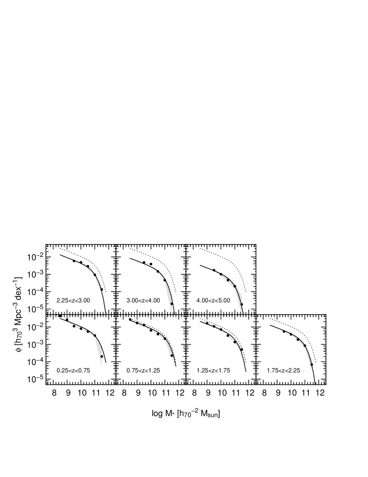
Figure 1.— The stellar mass function (MF) as a function of redshift. Data are from the Fors Deep Field (Drory et al., 2005). Schechter-fits to the data are over plotted as solid lines. Confidence regions are indicated by shading (random uncertainties only). The low-$z$ MF is repeated in the higher-$z$ panels for comparison.

where we have left out the arguments for brevity and divided by $\phi$ to obtain an equation for the relative change.

Note that (tidal) stripping of stars from a galaxy (e.g. in clusters or in interactions) contributes to eq. 3 as well. Assuming that this loss of stellar mass is small compared to the overall growth rate of a galaxy, it can be neglected.

The assembly rate is given in terms of the change in number density per unit time rather than in number of discrete merging events per object per unit time (and per unit merger mass ratio). Therefore, we can only speak of an effective merger rate, equivalent in its effect on the number density to an equal number of same-mass mergers per unit time interval. An alternative is to think about this quantity as simply representing the average effective mass accretion rate. We cannot discern the mass spectrum of accretion and merging events that actually cause the observed change in the mass function. It is also important to point out that a value of zero does not imply that no accretion and merging are happening, but only that the mass flux entering a mass bin through merging and the mass flux leaving that same mass bin through merging are equal, and hence the number density at this mass does not change. Values below zero imply that the number density decreases due to merging activity, and hence objects are preferably being accreted onto more massive objects and thus destroyed. To emphasize the difference between what we measure and the merger rate expressed as the number of merger events per unit time and object, we will avoid using the term merger rate and prefer the name assembly rate.

In the following sections we shall compile the necessary terms from GSMF and star formation data available in the literature. We will concentrate on the methodology and defer discussing selection effects and other deficiencies in the data to a later section where we proceed to plot eq. (3) and present our overall results.

3. The Galaxy Stellar Mass Function

The time derivative of the galaxy stellar mass function can be obtained in a fairly straight-forward way from observational studies of the GSMF. Here, we use the stellar mass function data spanning $0<z<5$ by Drory et al. (2005) from the Fors Deep Field (FDF).

The FDF photometric catalog is published in Heidt et al. (2003) and we use the I-band selected subsample covering the deepest central region of the field as described in Gabasch et al. (2004a). This catalog lists 5557 galaxies down to $I\sim 26.8$. The latter paper also shows that this catalog misses at most 10% of the objects found in ultra-deep K-band observations found by Labbé et al. (2003). Distances are estimated by photometric redshifts calibrated against spectroscopy up to $z\sim 5$ (Noll et al., 2004) providing an accuracy of $\Delta z/(z_{spec}+1)\leq 0.03$ with only $\sim 1$% outliers (Gabasch et al., 2004a). The spectroscopy samples objects statistically down to $I=25$.

The stellar masses are computed by fitting models of composite stellar populations of varying star formation history, age, metallicity, burst fractions, and dust content to UBgRIZJK multicolor photometry. We assume a Salpeter stellar initial mass function. At faint magnitudes, the uncertainties in the photometric distances are dominated by the large uncertainties in the colors. These are taken into account in the fitting procedure and hence reflected in the uncertainties in the individual masses entering the mass function. We refer the reader to the original publications for full details.

To lessen the impact of noise in the data on the time derivatives we are interested in, we choose to parameterize the evolution of the mass function, which we assume to be of Schechter form, by the following relations:

$$\phi(M)\,\mathrm{d}M\;=\;\phi^{*}\,\left(\frac{M}{M^{*}}\right)^{\alpha}\,\exp\left(-\frac{M}{M^{*}}\right)\frac{\mathrm{d}M}{M^{*}}\,,$$

and

$$\phi^{*}(z) \;=\; p_{1}\,(1+z)^{p_{2}}\,,$$ (4)

$$\log M^{*}(z) \;=\; q_{1}+q_{2}\,\ln(1+z)\,,$$ (5)

$$\alpha(z) \;=\; \alpha_{0}\,.$$ (6)

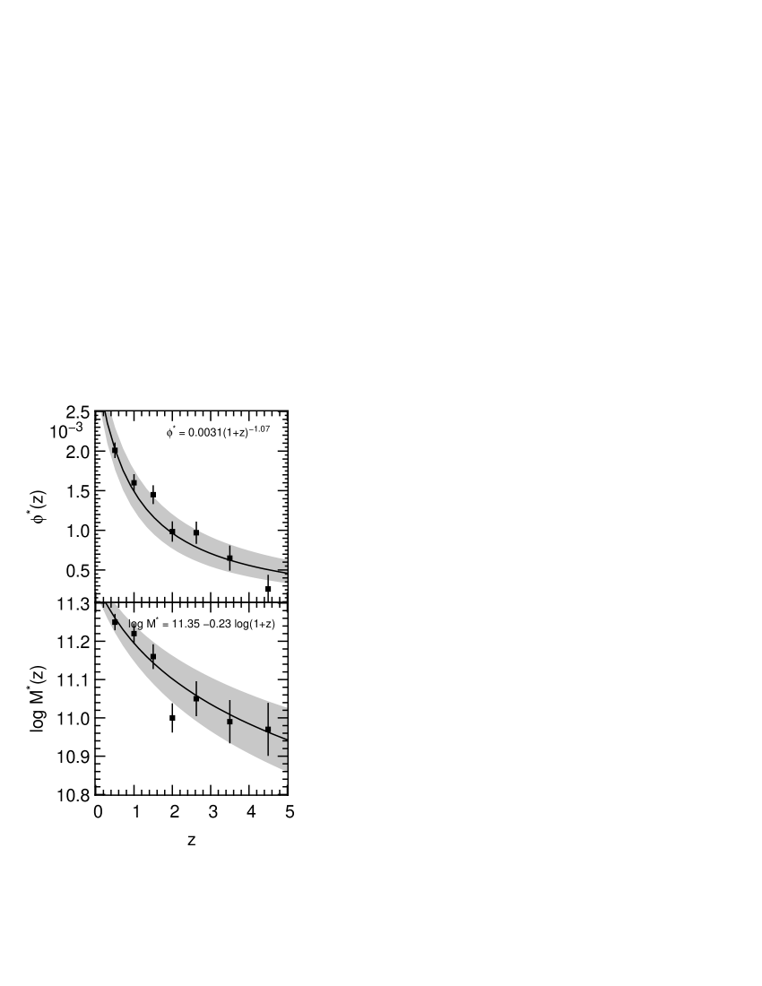
Figure 2.— Evolution with redshift of the parameters $\phi^{*}$ and $M^{*}$ of the Schechter functions fit to the data shown in Fig. 1. The shaded areas show the 1-$\sigma$ confidence region of the fit as determined from Monte Carlo simulations (see text). Note that the derivatives w.r.t. $z$ have much smaller uncertainties than the values of $\phi^{*}(z)$ and $M^{*}(z)$ themselves.

First, we fit individual Schechter functions to the data from Drory et al. (2005) in each redshift bin (Fig. 1). Then we fit eqs. (5)–(7) to the Schechter parameters as a function of redshift, $\phi^{*}(z)$ and $\log M^{*}(z)$, to obtain a smooth description of the redshift evolution of the stellar mass function (Fig. 2). The error bars of each data point are used to weight the data during fitting. We determine confidence intervals for $\phi^{*}(z)$ and $\log M^{*}(z)$ by Monte Carlo simulations. These confidence regions are indicated by shaded regions in Fig. 2. A consequence of parameterizing $\phi^{*}(z)$ and $\log M^{*}(z)$ in this way is that in spite of the large uncertainties of these quantities, the constraints on their derivatives with respect to time are a lot tighter.

In the redshift range $0<z\lesssim 2$, where the mass function data are deep enough to constrain the faint-end slope of the mass function, $\alpha$, it turns out to be consistent with being constant at $\alpha=-1.3$. At higher redshift, the data do not allow to constrain the faint-end slope any more. This is consistent with the results by Fontana et al., 2006.

We therefore fix alpha at its low-$z$ value for all redshifts. The consequences of this will be discussed below.

The mass function and the Schechter-fits to the data are shown in Fig. 1, and the best-fitting Schechter parameters are listed in Table 1. The fit to the evolution of the mass function with redshift as parameterized by eqs. (5)–(7) is shown in Fig. 2. The best fitting parametrization is

$$\phi^{*}(z) \;=\; (0.0031\pm 0.0002)\,(1+z)^{-1.07\pm 0.13}\,,$$

$$\log M^{*}(z) \;=\; (11.35\pm 0.04)-(0.22\pm 0.03)\,\ln(1+z)\,,$$

$$\alpha(z) \;=\; -1.3\,,$$

and we will use this form in the following.

Table 1Schechter fit parameters to the mass function

$z$	$\phi^{*}$	$\log M^{*}$	$\alpha$
	$h_{70}^{3}\,\mathrm{Mpc}^{-3}\,\mathrm{dex}^{-1}$	$h_{70}^{-2}\,\mathrm{M_{\sun}}$
0.50	$(2.01\pm 0.10)\times 10^{-3}$	$11.25\pm 0.02$	-1.3
1.00	$(1.60\pm 0.12)\times 10^{-3}$	$11.22\pm 0.03$	-1.3
1.50	$(1.45\pm 0.14)\times 10^{-3}$	$11.16\pm 0.03$	-1.3
2.00	$(9.85\pm 1.12)\times 10^{-4}$	$11.00\pm 0.04$	-1.3
2.75	$(9.70\pm 1.32)\times 10^{-4}$	$11.05\pm 0.04$	-1.3
3.50	$(6.50\pm 1.50)\times 10^{-4}$	$10.99\pm 0.05$	-1.3
4.50	$(2.61\pm 1.71)\times 10^{-4}$	$10.97\pm 0.07$	-1.3

Using this best-fitting parametrization of the evolution of the mass function, we can extrapolate the values of the parameters to $z=0$. We obtain $\phi^{*}(0)=0.0031~{}h_{70}^{3}\,\mathrm{Mpc}^{-3}\,\mathrm{dex}^{-1}$, which is consistent with the values obtained by Cole et al. (2001) (0.003) and Bell et al. (2003) (0.0034) when these are rescaled to the same initial mass function and cosmology. The value we obtain for the characteristic mass, $\log M^{*}(0)=11.35$, is higher than the values obtained in the mentioned literature (11.16 and 11.01, respectively); however, our value of the faint-end slope, $\alpha$, is different ($-1.3$ in this work as opposed to $-1.1$ in Cole et al., 2001 and $-1.18$ in Bell et al., 2003). If one takes the coupling between $M^{*}$ and $\alpha$ into account, a smaller value of $\alpha$ is degenerate with a higher value of $M^{*}$, and therefore our values agree very well with the literature at zero redshift, once “corrected” to the same $\alpha$ along the lines of the degeneracy.

In any case, the focus of this paper is to establish a method of disentangling star formation and merging contributions to galaxy stellar mass assembly. We shall therefore not be concerned too much about peculiarities of the mass function, instead we refer the interested reader to the relevant literature (e.g. Bell et al., 2003; Drory et al., 2005; Conselice et al., 2005; Fontana et al., 2006, and references therein).

4. The Average Star Formation Rate

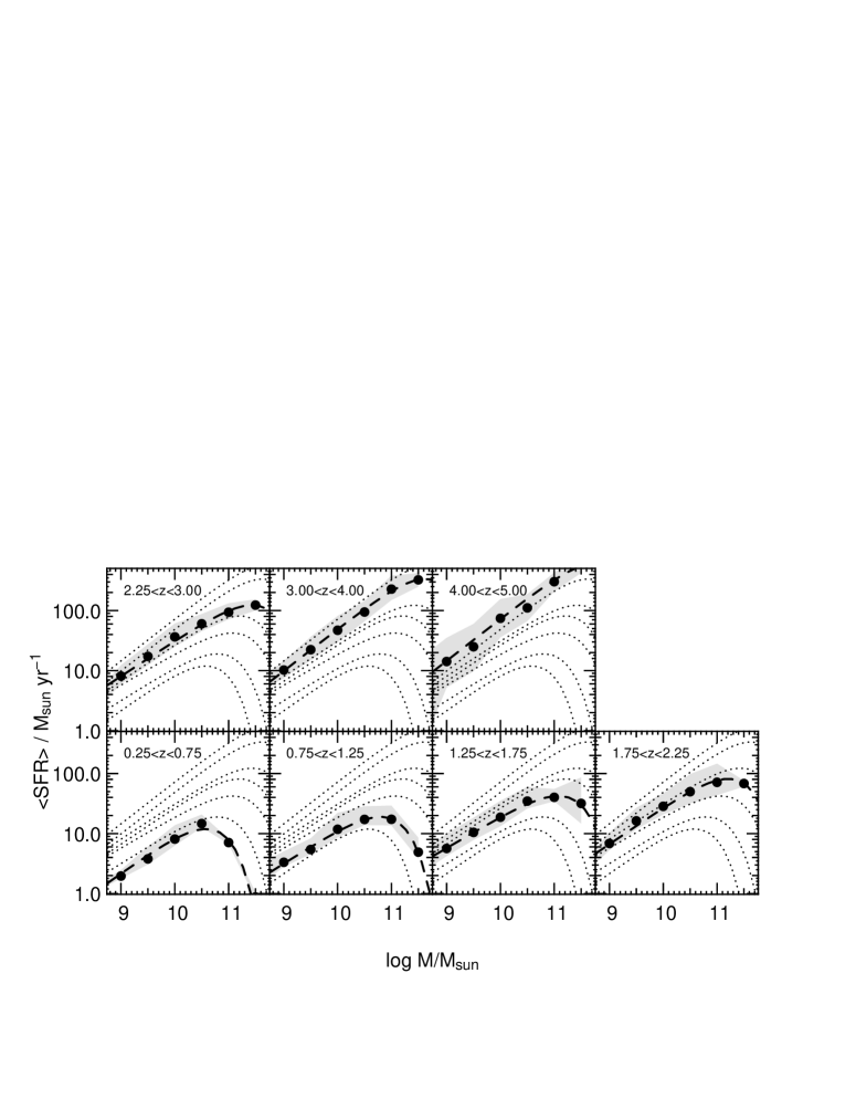
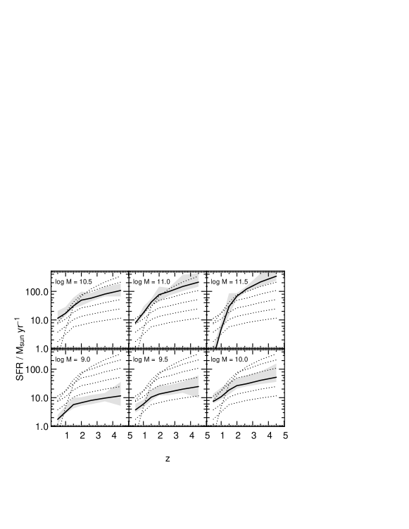
Figure 3.— The upper plot shows the average star formation rate as a function of stellar mass in seven redshift bins ranging $0.5<z<4.5$. Each panel shows the data of one redshift bin (filled circles). The confidence regions are indicated by shading. Fitting functions to the data (power laws with exponential cutoff at high mass; see text) are plotted as dashed lines. Each panel also shows the fitting functions in all other redshift bins as dotted lines for comparison. The lower plot shows the same data plotted against redshift. Each panel shows the star formation rate for a different stellar mass as a thick solid line. The dotted lines indicate the data for the other masses for comparison. Confidence regions are shaded.

To find the (average) star formation rate at each stellar mass and time, we take advantage of the data published by Feulner et al. (2005a) in the Fors Deep Field.

We use dust-corrected UV-continuum emission around 2800Å to estimate star formation rates. The reason for doing so is twofold. First, there are no other homogeneous datasets that provide more robust star formation rates over the whole redshift range of interest. Second, the UV continuum luminosity can be measured for every galaxy that has a stellar mass assigned to it. Therefore we have star formation rates for the exact same sample that is used to measure the stellar mass function. This at least provides some assurance of internal consistency.

Table 2Fit parameters to the star formation rate (Eq. 7)

$z$	$\dot{M}_{\ast}^{0}$	$\log M_{\ast}^{1}$	$\beta$
	$\mathrm{M_{\odot}}\,\mathrm{yr}^{-1}$	$\mathrm{M_{\odot}}$
0.50	$13.1\pm 1.6$	$10.77\pm 0.08$	$0.69\pm 0.11$
1.00	$20.1\pm 1.0$	$11.04\pm 0.04$	$0.56\pm 0.08$
1.50	$43.6\pm 2.8$	$11.35\pm 0.09$	$0.52\pm 0.07$
2.00	$88.2\pm 3.1$	$11.41\pm 0.11$	$0.61\pm 0.07$
2.75	$132\pm 3.9$	$11.67\pm 0.13$	$0.59\pm 0.05$
3.50	$336\pm 12.7$	$11.78(-0.25+\infty)$	$0.63\pm 0.02$
4.50	$576\pm 26.7$	$12.95(-0.31+\infty)$	$0.66\pm 0.01$

The dust corrections are estimated from the stellar population model fits to the multicolor photometry (see details and discussion in Feulner et al., 2005a).

How reliable are the UV-based star formation rates? Daddi et al. (2007) analyze multi-wavelength data (optical-NIR, Spitzer mid-IR, and radio) at $1.4<z<2.5$ in the GOODS region (see also Daddi et al., 2005). They conclude that the SFR can be estimated consistently from the UV light using SED or color-based dust corrections, with the UV-based estimates being within a factor of $\sim 2$ of the $24~{}\mu\mathrm{m}$-based estimate for most galaxies (Sub-mm galaxies are an exception, as for those, the UV underestimates the SFR by at least an order of magnitude, but these are likely missed by the I-band selected sample used here). At high IR luminosities the difference is higher, but it is often unclear whether it is due to an IR excess due to an AGN, which is likely because the UV estimate is in agreement with the radio-based estimate of the SFR. These conclusions are also supported by a similar analysis by Reddy et al. (2005). These data only probe relatively massive galaxies, though.

To estimate errors (or rather the range of possible values) of the average star formation rate as a function of mass, we proceed as following: instead of applying a further upward correction to all our star formation rates, we set the likely upper envelope of the average star formation rate as the average value plus the width of the distribution above the average (using the 68-percentile). The reasoning behind this is that the brightest UV sources at each mass are likely the least extinct ones, and therefore they mark the upper limit. The likely lower confidence limit on the average star formation rate is calculated by estimating the maximum amount by which the average might be lowered due to low-SFR galaxies missing in the sample. To do this we need to assume a distribution of star formation rates in objects below our detection limit. We assume a star formation rate function power-law slope of $-1.45$ following the only measurement by Bell et al. (2007). Note, though, that this measurement is at $z\lesssim 1$. We normalize to our mean densities and assume that the undetected population follows a power-law distribution of star formation rate of that slope at any given constant stellar mass and redshift. We then integrate the star formation rate function up to the point at which the objects would reach the detection limit of the FDF. The amount by which this missed star formation lowers the average value at each mass and redshift then defines the lower confidence limit. The region of confidence is shaded in Fig. 3.

To reduce the influence of noise in the data on the derivatives we are interested in, we will parameterize the average star formation rate as a function of mass by an analytic expression, just as we have done with the mass function. We choose a power law of the stellar mass with an exponential cutoff at high mass:

$$\dot{M}_{\ast}(M_{\ast})\;=\;\dot{M}_{\ast}^{0}\,\left(\frac{M_{\ast}}{M_{\ast}^{1}}\right)^{\beta}\,\exp\left(-\frac{M_{\ast}}{M_{\ast}^{1}}\right)\,.$$ (7)

The data along with this fit are shown in Fig. 3. The best-fitting parameters are listed in Table 2. Since such data on the star formation rate as a function of stellar mass and time have not been shown before in this form in the literature, we will take the time to digress from our goal of determining the assembly rate and discuss the star formation rate as it provides valuable insights.

A few regularities in the data are apparent. At $z\gtrsim 3$ the star formation rate monotonically rises with stellar mass to the highest masses we probe ($\log M_{\ast}\sim 11.5$). It is consistent with a single power law with exponent $\beta\sim 0.6$. The star formation rates in the most massive objects at this high redshift are of the order of 100 – 500 $\mathrm{M_{\odot}}\mathrm{yr}^{-1}$, suggesting that these are the progenitors of modern day massive ellipticals seen during their major epoch of star formation. The average star formation rate drops most rapidly with redshift for high mass ($\log M_{\ast}\gtrsim 11$) galaxies. Their period of active growth by star formation seems to be over by $z\sim 1.5$, and the star formation rate as a function of stellar mass turns over from increasing with mass to rapidly decreasing with both mass and time in objects with $\log M_{\ast}\gtrsim 11$.

At redshift $z\sim 3$, the star formation rates begin to drop at the high mass end while still being an increasing function of mass at lower masses. As redshift decreases further, the star formation rates drop at progressively lower masses. This behavior, usually termed downsizing (Cowie et al., 1996), has been observed in numerous recent high-redshift studies (e.g. Bauer et al., 2005; van der Wel et al., 2005; Bundy et al., 2006; Noeske et al., 2007a) and is also seen in studies of the fossil record of the stellar populations in the local universe (e.g. Heavens et al., 2004; Thomas et al., 2005). The mass at which the star formation rate starts to deviate from the power law form progresses smoothly from $\log M_{\ast}^{1}\sim 13$ at $z\sim 5$ to $\log M_{\ast}^{1}\sim 10.5$ at $z\sim 0.5$. For comparison, in the local universe Kauffmann et al. (2003b) find a characteristic mass of $\log M_{\ast}\sim 10.4$ at which the galaxy population changes from actively star forming at lower stellar mass to typically quiescent at higher masses. This transition mass shows a smooth evolution to higher masses at earlier times up to very high redshift (at $\gtrsim 3$ the data are consistent with a single power law and no break mass at all).

Figure 4.— Evolution of the characteristic mass, $M_{\ast}^{1}$, above which the star formation rate as a function of mass begins to drop.

How does this “break mass” – the mass above which the average star formation rate begins to decline – evolve with redshift? Fig. 4 shows the evolution of the parameter $M_{\ast}^{1}$ from eq. (7) against redshift, as well as a power-law fit to it:

$$M_{\ast}^{1}(z)=2.7\times 10^{10}(1+z)^{2.1}\,.$$ (8)

This can be compared directly to the result obtained from the SDSS sample in the local universe by Kauffmann et al. (2003b) (compare also Brinchmann et al., 2004). They find that above a stellar mass of $3\times 10^{10}~{}\mathrm{M_{\odot}}$, the fraction of galaxies with old stellar populations and low star formation rapidly increases. Our estimate of the zero redshift break mass in the star formation rate is $M_{\ast}^{1}(0)=2.7\times 10^{10}~{}\mathrm{M_{\odot}}$. Bundy et al. (2006) find evidence for an evolving mass limit for star forming galaxies in the DEEP2 redshift survey at $0.4<z<1.4$. Their best-fitting parametrization of the “quenching mass”, $M_{Q}(z)\propto(1+z)^{3.5}$, is probably comparable to ours given the difference in methodology and redshift range, although the exponent we find is somewhat smaller.

In the lower panels of Fig. 3, we plot the star formation rate against redshift for different fixed stellar masses. From this plot it is apparent that while massive galaxies have the highest (absolute) star formation rates, their star formation rates drop earlier and quicker than for lower stellar mass objects. The star formation rate in $\log M_{\ast}\sim 11$ objects drops by a factor $\sim 200$ between $z\sim 4.5$ and $z\sim 1$, while objects of $\log M_{\ast}\sim 9.5$ decrease their average star formation rate only by a factor $\sim 5$. Most of the latter decrease happens at $z\lesssim 1$. At higher redshifts, low mass galaxies have almost constant (average) star formation rates. The more rapid decline we find in the star formation rate of massive galaxies is in contrast with the analysis by Zheng et al. (2007) who combine $24~{}\mu\mathrm{m}$ data with UV data in the COMBO-17 survey and conclude that the star formation rate declines independently of galaxy mass at $z<1$ (using stacked detections to account for the average star formation rate in sources individually undetected at $24~{}\mu\mathrm{m}$). This difference could be due to the (SED-based dust corrected) UV light underestimating the true star formation rate in $\log M_{\ast}\gtrsim 11$ galaxies at $z<1$ more so than at lower masses. Another possibility is some uncertainty in the infrared SEDs of these galaxies and the calibration of the observed-frame $24~{}\mu\mathrm{m}$-based star formation rate at intermediate redshifts.

Another fact to note is that the exponent of the star formation rate as a function of stellar mass at masses below the break mass is remarkably stable. In all redshift bins, the exponent is close to $\beta\sim 0.6$, possibly steepening slightly to $\beta\sim 0.7$ at $z\lesssim 0.5$. This also means – since the exponent is always smaller than one – that the specific star formation (star formation rate per unit stellar mass) rate is a monotonically decreasing function of stellar mass at all masses and redshifts.

How does this compare to other studies of star formation rates? In the local universe, Brinchmann et al. (2004) find a very similar slope of the star formation rate with stellar mass as well ($\log\dot{M}_{\ast}\propto 0.6\,\log M_{\ast}$).

At intermediate redshift, in fact, Noeske et al. (2007b) argue for the existence of a “main sequence” of star forming galaxies that obeys the relation $\log\dot{M}_{\ast}=(0.67\pm 0.08)\,\log M_{\ast}-(6.19\pm 0.78)$ at $0.2<z<0.7$ and $10<\log M_{\ast}/\mathrm{M_{\odot}}<11$ using DEEP2 survey data combining $24~{}\mu\mathrm{m}$ and optical emission line fluxes. This is in very good agreement with our results. They also see indications of slight flattening towards higher redshift, although this cannot be said with confidence from their sample.

Papovich et al. (2006) studied massive galaxies at $1\lesssim z\lesssim 3.5$ detected by the Spitzer Space Telescope at $3-24~{}\mu\mathrm{m}$, by HST, and in ground based observations in the GOODS field. They also find a relation between stellar mass and star formation rate, and although they do not attempt to quantify this relation, their data is consistent with the relation proposed here. They also compare their high-$z$ results to similarly measured star formation rates in $z\lesssim 1$ galaxies selected from COMBO-17 and find similar results to the evolution presented here.

Also, our star formation rates (and stellar masses) in the Lyman break galaxy regime agree very well with detailed studies of this class of objects. As in Papovich et al. (2001), we find stellar masses of $9.5\lesssim\log M_{\ast}\lesssim 10.5$ and star formation rates (at $z\sim 3$) between 10 and 100 $\mathrm{M_{\odot}}\mathrm{yr}^{-1}$.

We are therefore confident that our relationship between stellar mass and star formation rate is robust and likely to be valid in spite of its rather simplistic footing. It is understood that there is an underlying broad distribution of star formation rates and much intrinsic scatter around this relation, especially at higher redshift where one is likely to encounter massive starbursts. Also, the relation as shown here is only strictly valid for “star forming galaxies”, as quiescent objects (most notably at lower masses) are most likely to be undetected (however, they will be missing from both $\phi(M_{\ast})$ and $\dot{M}_{\ast}(M_{\ast})$ in the present study).

Figure 5.— Star formation histories of galaxies with mass between $10^{8}$ and $10^{11.5}$ $\mathrm{M_{\odot}}$, calculated by integrating the star formation rate as a function of mass and time (Fig. 3). .

Finally, given the average star formation rate field $\dot{M}_{\ast}(M_{\ast},t)$, we can ask what the star formation histories look like on average as a function of mass, i.e. we can ask for tracks along $\dot{M}_{\ast}$ and $t$ that solve the equations

$$\mathrm{d}M_{\ast}/\mathrm{d}t \;=\; \dot{M}_{\ast}(M_{\ast},t)$$

$$M_{\ast}(t_{0}) \;=\; M_{0}\,.$$

Figure 5 shows these solutions for masses $M_{0}$ at $t_{0}$ of $8\leq\log M_{\ast}\leq 11.5$. Note that $M_{0}$ and $t_{0}$ are defined as the mass and time at $z=4.5$. In interpreting these as star formation histories of galaxies, we assume that the dominant contribution to the growth of stellar mass is from star formation, i.e. we neglect growth by accretion and merging, which we will see is a reasonable approximation in the following sections.

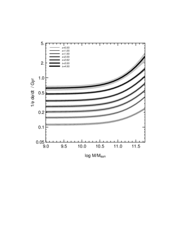
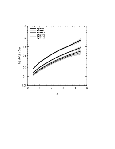
Figure 6.— The partial derivative with respect to time of the stellar mass function as measured from the parametrization of its redshift evolution (see text). The left hand panel shows the derivative as a function of stellar mass at different redshifts; thicker lines indicate higher $z$ with values between $z=0.5$ and $z=4.5$ as in Fig. 3. The right hand panel shows the same functions but plotted against redshift, with higher stellar mass indicated by thicker lines; the mass values are indicated and the same as in Fig. 3. At masses below $M^{*}$, where the mass function is a power law, the evolution becomes independent of mass. Therefore curves for masses below $\log M_{\ast}\sim 10$ in the right panel lie on top of each other.

It has long been thought that star formation histories of galaxies are roughly exponentials on average, with later type and lower mass galaxies having longer $e$-folding times (e.g. Sandage, 1986). From investigations of the present day stellar population in elliptical galaxies, this was confirmed by Thomas et al. (2005), at least for spheroidals. Heavens et al. (2004) use spectra of galaxies from the SDSS to infer star formation histories of galaxies as a function of mass and find similar trends. Here, Fig. 5 – from measurements of star formation rates as a function of stellar mass and redshift – directly shows that a relationship between star formation history and galaxy mass holds. Rise time, peak star formation rate, peak time, and post-maximum (exponential) decay timescale are all correlated with mass. More massive galaxies have steeper and earlier onsets of star formation, higher peak star formation rate, and the following exponential decay has a shorter $e$-folding time. Less massive galaxies have a more gradual onset of star formation, a broader peak of star formation activity, and their maximum star formation rate is lower and occurs later. Their subsequent exponential decline has a longer $e$-folding time.

Since the star formation rate as a function of mass is well represented by a power law in mass with constant slope, we can write the early star formation rate (at masses below the break mass) as $\mathrm{d}M/\mathrm{d}t=A(t)\,M^{\beta}$, with $A(t)\propto\dot{M}_{\ast}^{0}$ from eq. (7), and monotonically decreasing with time. Hence, galaxies which begin forming stars later in time, have longer rise times, reach lower peak star formation rate, and also lower final mass. The latter statement can be derived from the fact that the break mass decreases with time, and so galaxies that start forming stars later have their star formation quenched at lower mass than galaxies that start forming stars early, when the break mass is still high.

As a side note, the existence of the curious universal power-law relation between star formation rate and stellar mass can be explained using disk galaxy scaling relations and the Schmidt-Kennicutt star formation law (Kennicutt, 1998a). If one takes the Schmidt-Kennicutt law to read $\Sigma_{\mathrm{SFR}}\propto\Sigma/\tau_{\mathrm{dyn}}$ (with $\Sigma$ denoting surface density and $\tau$ being the dynamical timescale, see Silk, 1997; Kennicutt, 1998b), then $\dot{M}_{\ast}\propto R^{2}\,\Sigma_{\mathrm{SFR}}\propto R^{2}\,\Sigma\,V/R\propto\Sigma\,V\,R$ (with $V$ denoting the characteristic velocity of the system and $R$ its radius). Using the virial relation we have $\dot{M}_{\ast}\propto M_{\ast}^{0.5}\,R^{0.5}$, which, with $M\propto R^{3}$, becomes $\dot{M}_{\ast}\propto M_{\ast}^{0.62}$. Using the disk scaling relations given in Mo et al. (1998) instead of the (halo) virial relation ($M\propto V_{c}^{3}$; $R_{d}\propto V_{c}$), one obtains $\dot{M}_{\ast}\propto M_{\ast}$ for average halo spin parameter and fraction of disk angular momentum. Both of these arguments assume a fixed scaling of cold gas surface density with total mass surface density.

5. The Time Derivative of the Mass Function

Now that we have assembled all the necessary data, we turn back to eq. (2). The right hand side of eq. (2) has two terms. The first is the observed time derivative of the mass function, the second one is the change with time induced in the mass function due to star formation. Here we will deal with the first term.

We use the parametrization of the evolution of the stellar mass function as established in § 3. From this parametrization, it is a straight forward procedure to calculate the time derivative $\partial\phi/\partial t$. For convenience, we will henceforth always measure time derivatives in terms of relative changes, $(1/\phi)\,(\partial\phi/\partial t)$. These are plotted against mass in the left hand panel of Fig. 6; we use thicker lines to indicate higher redshift. The right hand panel shows the same quantity, this time plotted against redshift, with line thickness indicating increasing stellar mass. We plot data for the same redshifts and masses as in Fig. 3.

The shaded regions indicate the 1-$\sigma$ confidence limits calculated using Monte Carlo simulations of the fit of the evolution of the mass function, eqs. (5) – (7) and Fig. 2 in § 3. It is important to note that while the uncertainties on the mass function itself are rather large, the parameterization of its evolution provides much smaller formal uncertainties on the derivative with respect to time that is of interest here.

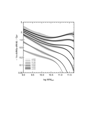
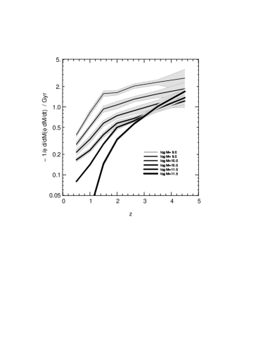
Figure 7.— The relative change per Gyr in the galaxy stellar mass function due to star formation only, plotted against mass (left panel) and redshift (right panel). These curves are the result of evaluating eq. 1. Confidence limits are derived by directly propagating the confidence limits on the average star formation rate through eq. 1.

Note that our parametrization of the mass function assumes a fixed faint-end slope of $\alpha=-1.3$ (the data do not allow us to measure the slope at higher redshift; up to $z\sim 2$, the slope is consistent with being constant). Hence the time derivative of the mass function becomes independent of mass at masses below the characteristic mass, $M^{*}(z)$, where the mass function is a power law. In the right hand panel of Fig. 6 this means that the low mass curves (below $\log M_{\ast}\sim 10$) all lie on top of each other.

The most rapid buildup of the mass function happens (not unexpectedly) at high redshift and at the high-mass end. At $z\sim 4$ and $\log M_{\ast}\sim 11$, the number density approximately doubles every Gyr, while the density of $\log M_{\ast}\sim 10$ objects (typical Lyman break galaxies) increases by 50% per Gyr. At $z\lesssim 1$, the change in number densities is much more modest, of the order of 10-20% per Gyr (and likely decreasing further rapidly), so that the mass density roughly doubles between $z\sim 1$ and $z=0$, a behavior observed and confirmed by many studies mentioned in the introduction.

There is rather little differential evolution in the Fors Deep Field stellar mass function in the sense that the ratio of the change at high mass and at low mass evolves from a factor of $\sim 4$ at high $z$ to a factor $\sim 2$ at $z\sim 0.5$. This has been noted in Drory et al. (2005); see their Fig. 4. Fontana et al. (2006), analyzing data similarly in the GOODS-MUSIC survey, find that this ratio tends to zero at late times, such that the buildup of the $\log M_{\ast}>11$ galaxy population is complete by $z\sim 1$ while it still continues slowly in our sample (compare also studies of elliptical galaxies, e.g. van der Wel et al., 2005). This discrepancy, apparent in a number of datasets – whether it is due to the small volume of the FDF at low $z$, the photometric redshifts, the stellar population modeling technique, or other effects – has yet to be resolved.

Since the main focus of this paper is to discuss the method presented here to analyze mass function and star formation rate data, we will not spend too much time discussing peculiarities of the present dataset. We are fully aware that the current data have significant deficiencies (both in mass and star formation rate), yet they still offer the possibility to discover and learn about fundamental trends in the formation and evolution of galaxies.

6. The Evolution of the Mass Function due to Star Formation

After the derivative of the mass function, we turn to the second term on the right hand side of eq. 2. We proceed to analyze the relative change in the stellar mass function that is due to star formation only, $\psi\equiv\frac{1}{\phi}\,\frac{\partial\phi(M_{\ast},t)}{\partial t}\Big{|}_{\mathrm{SF}}$, which is $\phi^{-1}$ times eq. 1. We will use the symbol $\psi$ to refer to this quantity in what follows.

To compute the function $\psi=\phi^{-1}\,(-\partial/\partial\,M_{\ast})\,\,(\phi\,\dot{M}_{\ast})$, in each time (redshift) bin, we use the parameterized fits to $\phi(M_{\ast},t)$ and $\dot{M}_{\ast}(M_{\ast},t)$ listed in Tables 1 and 2, respectively. We plot the resulting curves in Fig. 7. The left hand panel shows the relative change of the stellar mass function plotted against stellar mass in seven redshift bins spanning $0.5<z<4.5$; as in the previous plots, thicker lines indicate higher redshift. The right hand panel shows the same data but now plotted against redshift with stellar mass coded as line thickness. Masses and redshifts are the same as in Fig. 6. Confidence regions are derived directly from the confidence limits on the average star formation rates propagated through eq. 1.

$\psi(M_{\ast},t)$ is positive at all times. This means that the number density of galaxies is predicted to increase with time due to the star formation activity of the galaxies. Note that this is not a trivial statement: If the number of objects leaving a mass bin $[M_{\ast},M_{\ast}+\mathrm{d}M_{\ast})$ in the time interval $\mathrm{d}t$ due to their star formation rate $\dot{M}_{\ast}(M_{\ast},t)$ is larger than the number of objects entering the same bin from lower mass due to their own star formation (see eq. (1)), the number density at this mass would decrease. It is a matter of comparing the derivatives w.r.t. mass of the mass function and the star formation rate.

In the low-mass range, the stellar mass function is well represented by a power law with slope $\alpha\sim-1.3$ (locally), and we have assumed that this slope does not evolve with time (which is backed by the data up to $z\sim 2$; see § 3 and also Fontana et al., 2006). The star formation rate is also well described by a power law (see § 4), $\dot{M}_{\ast}\propto M_{\ast}^{\beta}$, with $\beta\sim 0.6$. Eq. (1) times $\phi^{-1}$ hence reduces to

$$\psi\propto-\frac{1}{M_{\ast}^{\alpha}}\,\frac{\partial}{\partial M_{\ast}}\,\left[M_{\ast}^{\alpha}\,M_{\ast}^{\beta}\right]\;\propto\;-(\alpha+\beta)\,M_{\ast}^{\beta-1}\,.$$ (9)

This term is positive if $\alpha+\beta<0$. With $\alpha\sim-1.3$ and $\beta\sim 0.6$, this condition is satisfied at all times at the faint end. At the bright end, the mass function steepens quicker than the star formation rate does, and the condition remains satisfied.

We wish to note here that we are very likely to miss low-mass low star formation part of the galaxy population, hence we very likely underestimate the slope of the stellar mass function, especially at higher redshift.

At high redshift and high mass, we see that star formation leads to a strong increase in number density. The number of objects with $\log M_{\ast}\gtrsim 11$ roughly doubles every Gyr at $z\sim 4$. This rate of buildup quickly decreases with time, slowing down to an increase by 50% per Gyr by $z\sim 2.5$. At $z\lesssim 1.5$, star formation has dropped to contribute a relative increase in number density of $\sim 0.1$ Gyr^-1, and to 0.05 Gyr^-1 at $z\sim 0.5$.

At low masses, $\log M_{\ast}\lesssim 10$, the number density very rapidly increases (due to star formation) at a rate comparable to that of high-mass objects. Unlike the high mass objects, however, the growth due to star formation persists in low mass objects for much longer, dropping to a rate of 0.5 Gyr^-1 at $z\sim 1$ and 0.2 Gyr^-1 at $z\sim 0.5$. While the number density of massive galaxies is not changing significantly anymore due to star formation at low $z$, that of low-mass galaxies does.

7. The Assembly Rate

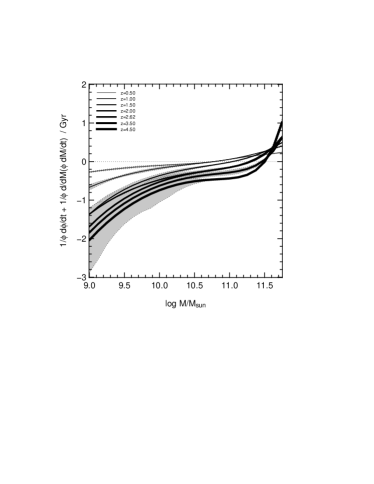
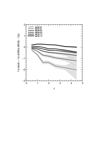
Figure 8.— The assembly rate: the relative change in the galaxy stellar mass function that is caused by anything other than star formation. We interpret this quantity as being due to accretion and merging of galaxies. The left hand panel is plotted against mass, the right hand panel against redshift.

Finally, we have all the ingredients necessary to fully evaluate eq. (3), which we do in Fig. 8, showing our results again versus mass in the left panel and against redshift in the right panel. We will use the less cumbersome term assembly rate for “change in number density due to merging” in what follows. We remind the reader to be mindful of the difference between this quantity and the merger rate (see § 2).

Confidence regions in Fig. 8 are calculated by means of Monte Carlo realizations of data within the uncertainties in the mass function evolution and the star formation rates, and propagating those through eq. (3). It is worth noting that since the constraints on the derivatives of $\phi^{*}$ and $\log M^{*}$ with respect to time are much tighter than the constraints on these quantities themselves, the error budget in Fig. 8 is dominated by the uncertainty in the average star formation rate. This leads to formally small errors at masses and redshifts with low star formation rates.

The curves in Fig. 8 are negative at low mass and positive at high mass, with the zero-crossing mass evolving from higher masses at high redshift to lower masses at lower redshift. This means that once star formation is accounted for, a source of high mass objects and a sink of low mass objects is necessary to explain the mass function data. In the most general terms, this is consistent with merging activity building up higher mass objects from (many) lower mass ones. In this picture, the merger rate decreases with time (the absolute value of the curves decreases with time). Also, the mass at which the merger rate tends to increase the number density instead of decreasing it (the mass above which objects are accreted onto and below which objects are destroyed) decreases with time. However, an important caveat is that a loss of objects could also be due to (faint) objects dropping out of the survey as soon as their star formation activity ceases. This can partly explain the negative values observed at low masses and the trend mentioned above.

In the following we shall look into the merger rates as a function of mass and time in more detail.

7.1. High redshift and high mass

At high redshift and high masses, the time-evolution in the mass function shows a rapid increase in number density of high mass objects (see § 5). Star formation accounts for most of this increase, leaving a difference consistent with zero at $\log M_{\ast}\sim 11$ and a small positive difference of $0.2-0.8$ Gyr^-1 at $\log M_{\ast}\sim 11.5$ and $z\gtrsim 3$. However, our parametrization of $\phi^{*}(z)$ flattens at high redshifts and over-predicts the normalization of the mass function in the bin at high $z$ (compare the high-$z$ data point in the upper panel of Fig. 2). As a result, the total change in the mass function is smaller in the parameterized fit to $\phi^{*}(z)$ compared to the raw data by about 30%. Therefore, if we use the Schechter functions shown in Fig. 1 directly, which show a steeper increase in $\phi^{*}$ at $z\gtrsim 3$, instead of the smooth parametrization $\phi^{*}\propto(1+z)^{-1.07}$, the curves in Fig. 8 move up, and the inferred assembly rate becomes larger by the same amount.

Given this uncertainty, we feel that the star formation rate we observe is roughly sufficient to explain the increase in number density at high mass and high redshift. As an upper limit, at most 0.5–0.8 effective major mergers per Gyr are consistent with the data. This number, though, would be enough to transform most of these early high mass objects into ellipticals contemporaneously with their major star formation episode. This is consistent with the picture emerging from various observations in the local universe and at high redshift which show that most massive ellipticals form quickly and early, with more massive galaxies being older, and their stars having formed more rapidly (e.g. Bender et al., 1996; Treu et al., 2001; van de Ven et al., 2003; Thomas et al., 2005; van der Wel et al., 2005; Renzini, 2006).

7.2. High redshift and low mass

As we have seen, the data point towards small galaxies being destroyed and large galaxies being built by mergers, with the caveat of selection effects being responsible for parts of this trend.

A plausible interpretation instead of invoking a high destruction rate due to mergers, is based on the fact that low mass objects with low star formation rates (and therefore redder colors) are very likely missing from the survey. If the slope of the mass function were steeper due to the existence of a class of low-mass objects missing from the survey, we’d need an even higher destruction rate at low masses, due to the increase in numbers and decrease in the average star formation rate. However, if the star formation rate as a function of mass were steeper, $\dot{M}_{\ast}\propto M_{\ast}^{0.8}$ instead of $\dot{M}_{\ast}\propto M_{\ast}^{0.6}$ either due to lower star formation at low masses or higher star formation at high masses, the difference would be close to zero below $\log M_{\ast}\sim 11$ at all times, and little change ($\sim 0.2$ Gyr^-1) in number density due to merging would be necessary. This would imply that at low masses, merging is creating objects of any particular mass at the same rate as these objects are incorporated into larger structures.

7.3. Low redshift and high mass

Our current dataset is most reliable (both in terms of mass completeness and robustness of the star formation rate estimate) at redshifts $z\lesssim 2$ and at masses $\log M_{\ast}\gtrsim 10.5$. Here, the photometric data are deep enough to detect objects over a large dynamic range in $M_{\ast}/L$, and, also, intergalactic absorption (the Lyman break) does not affect the optical bands yet, such that the object’s spectral energy distributions are well-sampled from the rest-frame UV into the optical and near-IR.

At $z\lesssim 2.5$ the assembly rate is increasing towards higher stellar masses and towards lower redshift, mostly due to the rapid decline of the star formation rate in this regime, but it is always very low. Most of the increase in number density of massive galaxies is fully explained by the star formation rates observed.

It is very difficult to measure the high mass end of the mass function accurately. These objects are rare, and on the steep exponential tail of the mass function any small error in distance (due to the use of photometric redshifts) or error in $M_{\ast}/L$ will lead to a large error in the number density. Also, the effects of cosmic variance are largest in this mass range and may heavily bias results especially in relatively small-area surveys as the FDF. Some assurance is provided by the fact that the $z\sim 1$ mass functions of a number of surveys agree reasonably well. If our measurement of the high mass end of the mass function at $z<1.5$ is correct, mergers only contribute to the growth of the mass function at $\log M_{\ast}\gtrsim 11$ and only on a low level. A growth of only 0.1 – 0.2 Gyr^-1 is consistent with our data. This is equivalent to about 1 effective major merger per object in the redshift range $1.5>z>0$. If, on the other hand, there is less evolution at the high mass end of the mass function, e.g. as found by Fontana et al. (2006), then no merging at all would be required at high mass (compare also the mass functions in Fontana et al., 2004 and Drory et al., 2004). However, there is strong observational evidence that recent merging does play a role at least in field elliptical galaxies (e.g. Schweizer, 1982; Whitmore et al., 1997; Goudfrooij et al., 2001; Genzel et al., 2001).

Other studies of the merger rate do not help to answer this question. On one side, van Dokkum (2005) studied signatures of interaction and tidal debris in a sample of nearby red galaxies. With some assumptions on the timescale of the merger events, they conclude that the present day accretion rate in E/S0 galaxies is $\Delta M/M=0.09\pm 0.04$ Gyr^-1, a value that is fully consistent with our measurement, assuming that red sequence galaxies comprise the majority of the $\log M_{\ast}>11$ local galaxy population. Also, Bell et al. (2006b) find that 50-70% of galaxies with $\log M_{\ast}>10.7$ have undergone a major merger since $z\sim 1$ (see also Bell et al., 2006a). On the other side, Lin et al. (2004) and Lotz et al. (2006) find a much lower merger rate. They argue that in the DEEP2 survey, only $\sim 10\%$ of massive galaxies have undergone a major merger since $z\sim 1.2$. Bundy et al. (2006) also argue for a low contribution of mergers at the high mass end. An overview of a number of studies is given in Kartaltepe et al. (2007).

7.4. Evolution with time

As we have mentioned, the general trend in the data is for the assembly rate to become more positive with time. The zero-crossing mass decreases with time. In high mass objects, the assembly rate starts out at zero or slightly below, with star formation rates dominating the initial increase in number density. The assembly rate then increases, such that at low $z$, merging becomes the dominant process that increases the number density at masses $\log M_{\ast}\gtrsim 11$. The growth rate in this mass and redshift range is 0.1 – 0.2 Gyr^-1. Lower-mass galaxies are consumed in these mergers. The mass at which the assembly rate transitions from objects being consumed to objects being formed decreases with time, roughly tracing the break mass in the star formation rate. The zero-crossing of the assembly rate occurs at $\log M_{\ast}=10.8$ at $z=0.5$, $\log M_{\ast}=11.0$ at $z=1.5$, $\log M_{\ast}=11.3$ at $z=2$, and $\log M_{\ast}=11.5$ at $z=3.5$. While merging is still happening below this transition mass, the net number of objects decreases there. Hence, at lower redshift, the number density of progressively lower-mass galaxies starts to increase due to merging. This is a direct observation of the top-down buildup of the red sequence, where major merger remnants are found (e.g. Bell et al., 2004; Faber et al., 2005; Bundy et al., 2006; Bell et al., 2007).

It is interesting to note that in CDM, e.g. in the Press & Schechter (1974) formalism, we expect the opposite behavior: the characteristic mass increases with time, and hence progressively more massive halos preferably get incorporated into even larger structures, and their number density begins to decline. However, this formalism assumes that merged halos do not survive as substructure within their parent halos. Accounting for the survival of substructure, e.g. the existence of satellite galaxies or galaxies within clusters, might account for this apparent discrepancy. This will be explored in a follow-up paper.

8. Summary, Discussion, and Conclusions

Summarizing our results, we present average star formation rates as a function of stellar mass and redshift, $\dot{M}_{\ast}(M_{\ast},t)$, for galaxies in the Fors Deep Field spanning $0<z<5$. We directly measure their star formation histories as a function of stellar mass by integrating the former quantity.

At $z\gtrsim 3$ the average star formation rate is monotonically rising with stellar mass and is well-fitted by a power law of stellar mass with exponent $\beta\sim 0.6$. The average star formation rates in the most massive objects at this redshift are 100 – 500 $\mathrm{M_{\odot}}\mathrm{yr}^{-1}$, suggesting that these are the progenitors of modern day massive ellipticals seen during their major epoch of star formation. At redshift $z\sim 3$, the star formation rates starts to drop at the high mass end while still being an increasing function of mass at lower masses. The power-law exponent is consistent with staying constant. As redshift decreases further, the star formation rates drop at progressively lower masses (downsizing), dropping most rapidly with redshift for high mass ($\log M_{\ast}\gtrsim 11$) galaxies. The mass at which the star formation rate starts to deviate from the power law form (break mass) progresses smoothly from $\log M_{\ast}^{1}\gtrsim 13$ at $z\sim 5$ to $\log M_{\ast}^{1}\sim 10.9$ at $z\sim 0.5$. For comparison, in the local universe Kauffmann et al. (2003b) find a characteristic mass of $\log M_{\ast}\sim 10.4$ at which the galaxy population changes from actively star forming at lower stellar mass to typically quiescent at higher masses. The break mass is evolving with redshift according to $M_{\ast}^{1}(z)=2.7\times 10^{10}(1+z)^{2.1}$.

We directly show that a relationship between star formation history and galaxy mass holds. Rise time, peak star formation rate, peak time, and post-maximum (exponential) decay timescale are all correlated with mass. More massive galaxies have steeper early onsets of star formation, their peak star formation occurs earlier and is higher, and the following exponential decay has a shorter $e$-folding time.

We then present a method to infer effective merger rates (or mass accretion rates) from observations of the galaxy stellar mass function and the star formation rate as a function of mass and time. We quantify the evolution of the mass function due to the star formation activity of galaxies. We compare this evolution to the observed time derivative of the mass function and interpret any difference between the two as due to changes in galaxy mass due to external causes; accretion and merging are dominant among such processes. We introduce and analyze a quantity that we call the assembly rate, which is defined as the change in number density of galaxies due to accretion and merging.

We observe sufficient star formation to explain the increase in number density at high mass and high redshift. As an upper limit, at most 0.8 effective major mergers per Gyr are consistent with the data. This number, though, would be enough to transform most of these high mass objects into ellipticals contemporaneously to their major star formation episode.

The data point towards small galaxies being destroyed and large galaxies being built by mergers, with the caveat of selection effects being responsible for parts of this trend. A plausible interpretation, instead of invoking a high destruction rate due to mergers, is based on the fact that low mass objects with low star formation rates (and therefore redder colors) are very likely missing from the survey. The general trend in the data is for the assembly rate to become more positive with time. The zero-crossing mass decreases with time. In high mass objects, the assembly rate starts out at zero or slightly below, with star formation rates dominating the initial increase in number density. The assembly rate then increases, such that at low $z$, merging becomes the dominant process that increases the number density at masses $\log M_{\ast}\gtrsim 11$. A growth of 0.1 – 0.2 Gyr^-1 is consistent with our data at $z\lesssim 1.5$. This is equivalent to about 1 effective major merger per object in the redshift range $1.5>z>0$.

Synthesizing the above into a picture of the formation of massive ellipticals, a picture can be drawn in which elliptical galaxies would have formed their stars quickly and early ($z\gtrsim 2.5$) and subsequently quenched their star formation, with the highest mass galaxies forming first, and on the shortest timescale. Their elliptical morphology may be a consequence of early merging activity given the merger rate that is consistent with our data at high redshift ($\sim 0.8$ Gyr^-1; see above). Later, these galaxies may continue to evolve along the red sequence, however during this phase at $z\lesssim 1.5$, not much growth by merging is happening any more (at most a factor of two in stellar mass).

At more moderate masses of $10<\log M_{\ast}<11$, we find that the evolution of the number density due to mergers points towards these galaxies being preferably destroyed at early times, while at later times the change in their numbers turns positive. At lower redshift, the number density of progressively lower mass galaxies starts to increase due to merging. This is a direct confirmation of the top-down buildup of the red sequence suggested by recent observations (e.g. Bell et al., 2004; Faber et al., 2005; Bundy et al., 2006; Bell et al., 2007) and the simultaneous shutdown of star formation in these objects.

The results presented here do depend on some assumptions that we had to make, mainly due to general deficiencies of current observations and more specifically of the dataset we have at hand. Assuming that the faint-end slope of the MF does not evolve is consistent with the observations only up to $z\lesssim 2$ (Drory et al., 2005; Fontana et al., 2006). A steeper faint-end slope is possible due to faint objects (with lower star formation rates than the detected ones) being missed due to the survey flux limit. Therefore, a steeper faint-end slope of the MF also means a flatter average star formation rate, and hence a larger assembly rate at low masses.

The fitting function one chooses to use to describe the evolution of the mass function also affects the results. For example, a power-law fit to the evolution of $\phi^{*}$ constrains the derivative of the MF w.r.t. time, and thus limits the possible range of assembly rates. Ideally, one would like to have MF data robust enough to be used to measured derivatives directly and avoid the use of fitting formulae entirely.

The choice of a single average value for the SFR at each mass and redshift also affects the results. In reality, galaxies show a range of activity at fixed mass. Allowing for such a range of possible values instead of a single number would lend the method more flexibility, but also demands much higher quality star formation data with better-understood selection effects.

The current generation of ongoing large-area surveys offer the possibility to further explore the build up of the red sequence. With a much larger number of red and massive objects, one could improve on the analysis presented above in various ways. Studying merger processes as a function of the environment is one such possibility. Another promising approach is to separate galaxies into passive objects and objects that are actively forming stars. One can then apply our method to these two classes of objects individually, adding another term to eq. (3) that describes the rate of migration between the two sequences. This will allow to investigate the relation between merging activity and quenching of star formation in a very direct way.

References

- Bauer et al. (2005) Bauer, A. E., Drory, N., Hill, G. J., & Feulner, G. 2005, ApJ, 621, L89
- Bell et al. (2003) Bell, E. F., McIntosh, D. H., Katz, N., & Weinberg, M. D. 2003, ApJS, 149, 289
- Bell et al. (2006a) Bell, E. F., et al. 2006a, ApJ, 640, 241
- Bell et al. (2005) Bell, E. F., et al. 2005, ApJ, 625, 23
- Bell et al. (2006b) Bell, E. F., Phleps, S., Somerville, R. S., Wolf, C., Borch, A., & Meisenheimer, K. 2006b, ApJ, 652, 270
- Bell et al. (2004) Bell, E. F., et al. 2004, ApJ, 608, 752
- Bell et al. (2007) Bell, E. F., Zheng, X. Z., Papovich, C., Borch, A., Wolf, C., & Meisenheimer, K. 2007, ArXiv e-prints, 704
- Bender et al. (1996) Bender, R., Ziegler, B., & Bruzual, G. 1996, ApJ, 463, L51
- Borch et al. (2006) Borch, A., et al. 2006, A&A, 453, 869
- Bouwens et al. (2006) Bouwens, R. J., Illingworth, G. D., Blakeslee, J. P., & Franx, M. 2006, ApJ, 653, 53
- Brinchmann et al. (2004) Brinchmann, J., Charlot, S., White, S. D. M., Tremonti, C., Kauffmann, G., Heckman, T., & Brinkmann, J. 2004, MNRAS, 351, 1151
- Brinchmann & Ellis (2000) Brinchmann, J., & Ellis, R. S. 2000, ApJ, 536, L77
- Bundy et al. (2005) Bundy, K., Ellis, R. S., & Conselice, C. J. 2005, ApJ, 625, 621
- Bundy et al. (2006) Bundy, K., et al. 2006, ApJ, 651, 120
- Bundy et al. (2004) Bundy, K., Fukugita, M., Ellis, R. S., Kodama, T., & Conselice, C. J. 2004, ApJ, 601, L123
- Burkey et al. (1994) Burkey, J. M., Keel, W. C., Windhorst, R. A., & Franklin, B. E. 1994, ApJ, 429, L13
- Carlberg et al. (2000) Carlberg, R. G., et al. 2000, ApJ, 532, L1
- Chapman et al. (2005) Chapman, S. C., Blain, A. W., Smail, I., & Ivison, R. J. 2005, ApJ, 622, 772
- Cohen (2002) Cohen, J. G. 2002, ApJ, 567, 672
- Cole et al. (2001) Cole, S., et al. 2001, MNRAS, 326, 255
- Conselice (2006) Conselice, C. J. 2006, ApJ, 638, 686
- Conselice et al. (2005) Conselice, C. J., Blackburne, J. A., & Papovich, C. 2005, ApJ, 620, 564
- Cowie et al. (1996) Cowie, L. L., Songaila, A., Hu, E. M., & Cohen, J. G. 1996, AJ, 112, 839
- Daddi et al. (2005) Daddi, E., et al. 2005, ApJ, 631, L13
- Daddi et al. (2007) Daddi, E., et al. 2007, ApJ, 670, 156
- De Propris et al. (2005) De Propris, R., Liske, J., Driver, S. P., Allen, P. D., & Cross, N. J. G. 2005, AJ, 130, 1516
- Dickinson et al. (2003) Dickinson, M., Papovich, C., Ferguson, H. C., & Budavári, T. 2003, ApJ, 587, 25
- Drory et al. (2004) Drory, N., Bender, R., Feulner, G., Hopp, U., Maraston, C., Snigula, J., & Hill, G. J. 2004, ApJ, 608, 742
- Drory et al. (2001) Drory, N., Bender, R., Snigula, J., Feulner, G., Hopp, U., Maraston, C., Hill, G. J., & de Oliveira, C. M. 2001, ApJ, 562, L111
- Drory et al. (2005) Drory, N., Salvato, M., Gabasch, A., Bender, R., Hopp, U., Feulner, G., & Pannella, M. 2005, ApJ, 619, L131
- Eyles et al. (2007) Eyles, L. P., Bunker, A. J., Ellis, R. S., Lacy, M., Stanway, E. R., Stark, D. P., & Chiu, K. 2007, MNRAS, 374, 910
- Faber et al. (2005) Faber, S. M., et al. 2005, ArXiv Astrophysics e-prints
- Feulner et al. (2005a) Feulner, G., Gabasch, A., Salvato, M., Drory, N., Hopp, U., & Bender, R. 2005a, ApJ, 633, L9
- Feulner et al. (2005b) Feulner, G., Goranova, Y., Drory, N., Hopp, U., & Bender, R. 2005b, MNRAS, 358, L1
- Feulner et al. (2006) Feulner, G., Hopp, U., & Botzler, C. S. 2006, A&A, 451, L13
- Flores et al. (1999) Flores, H., et al. 1999, ApJ, 517, 148
- Fontana et al. (2003) Fontana, A., et al. 2003, ApJ, 594, L9
- Fontana et al. (2004) Fontana, A., et al. 2004, A&A, 424, 23
- Fontana et al. (2006) Fontana, A., et al. 2006, A&A, 459, 745
- Gabasch et al. (2004a) Gabasch, A., et al. 2004a, A&A, 421, 41
- Gabasch et al. (2004b) Gabasch, A., et al. 2004b, ApJ, 616, L83
- Genzel et al. (2001) Genzel, R., Tacconi, L. J., Rigopoulou, D., Lutz, D., & Tecza, M. 2001, ApJ, 563, 527
- Glazebrook et al. (2004) Glazebrook, K., et al. 2004, Nature, 430, 181
- Gottlöber et al. (2002) Gottlöber, S., Kerscher, M., Kravtsov, A. V., Faltenbacher, A., Klypin, A., & Müller, V. 2002, A&A, 387, 778
- Gottlöber et al. (2001) Gottlöber, S., Klypin, A., & Kravtsov, A. V. 2001, ApJ, 546, 223
- Goudfrooij et al. (2001) Goudfrooij, P., Mack, J., Kissler-Patig, M., Meylan, G., & Minniti, D. 2001, MNRAS, 322, 643
- Governato et al. (1999) Governato, F., Gardner, J. P., Stadel, J., Quinn, T., & Lake, G. 1999, AJ, 117, 1651
- Grazian et al. (2007) Grazian, A., et al. 2007, A&A, 465, 393
- Heavens et al. (2004) Heavens, A., Panter, B., Jimenez, R., & Dunlop, J. 2004, Nature, 428, 625
- Heidt et al. (2003) Heidt, J., et al. 2003, A&A, 398, 49
- Hopkins & Beacom (2006) Hopkins, A. M., & Beacom, J. F. 2006, ApJ, 651, 142
- Juneau et al. (2005) Juneau, S., et al. 2005, ApJ, 619, L135
- Kartaltepe et al. (2007) Kartaltepe, J. S., et al. 2007, ApJS, 172, 320
- Kauffmann et al. (2003a) Kauffmann, G., et al. 2003a, MNRAS, 341, 33
- Kauffmann et al. (2003b) Kauffmann, G., et al. 2003b, MNRAS, 341, 54
- Kennicutt (1998a) Kennicutt, R. C., Jr. 1998a, ARA&A, 36, 189
- Kennicutt (1998b) Kennicutt, R. C., Jr. 1998b, ApJ, 498, 541
- Labbé et al. (2003) Labbé, I., et al. 2003, AJ, 125, 1107
- Le Fèvre et al. (2000) Le Fèvre, O., et al. 2000, MNRAS, 311, 565
- Lilly et al. (1996) Lilly, S. J., Le Fèvre, O., Hammer, F., & Crampton, D. 1996, ApJ, 460, L1
- Lin et al. (2004) Lin, L., et al. 2004, ApJ, 617, L9
- Lotz et al. (2006) Lotz, J. M., et al. 2006, ArXiv Astrophysics e-prints
- Madau et al. (1996) Madau, P., Ferguson, H. C., Dickinson, M. E., Giavalisco, M., Steidel, C. C., & Fruchter, A. 1996, MNRAS, 283, 1388
- Madau et al. (1998) Madau, P., Pozzetti, L., & Dickinson, M. 1998, ApJ, 498, 106
- Mo et al. (1998) Mo, H. J., Mao, S., & White, S. D. M. 1998, MNRAS, 295, 319
- Nagamine et al. (2006) Nagamine, K., Ostriker, J. P., Fukugita, M., & Cen, R. 2006, ApJ, 653, 881
- Neuschaefer et al. (1997) Neuschaefer, L. W., Im, M., Ratnatunga, K. U., Griffiths, R. E., & Casertano, S. 1997, ApJ, 480, 59
- Noeske et al. (2007a) Noeske, K. G., et al. 2007a, ApJ, 660, L47
- Noeske et al. (2007b) Noeske, K. G., et al. 2007b, ApJ, 660, L43
- Noll et al. (2004) Noll, S., et al. 2004, A&A, 418, 885
- Pannella et al. (2006) Pannella, M., Hopp, U., Saglia, R. P., Bender, R., Drory, N., Salvato, M., Gabasch, A., & Feulner, G. 2006, ApJ, 639, L1
- Papovich et al. (2001) Papovich, C., Dickinson, M., & Ferguson, H. C. 2001, ApJ, in press
- Papovich et al. (2006) Papovich, C., et al. 2006, ApJ, 640, 92
- Patton et al. (2002) Patton, D. R., et al. 2002, ApJ, 565, 208
- Pei et al. (1999) Pei, Y. C., Fall, S. M., & Hauser, M. G. 1999, ApJ, 522, 604
- Pérez-González et al. (2003a) Pérez-González, P. G., Gallego, J., Zamorano, J., Alonso-Herrero, A., Gil de Paz, A., & Aragón-Salamanca, A. 2003a, ApJ, 587, L27
- Pérez-González et al. (2003b) Pérez-González, P. G., Gil de Paz, A., Zamorano, J., Gallego, J., Alonso-Herrero, A., & Aragón-Salamanca, A. 2003b, MNRAS, 338, 525
- Pérez-González et al. (2005) Pérez-González, P. G., et al. 2005, ApJ, 630, 82
- Pozzetti et al. (2007) Pozzetti, L., et al. 2007, A&A, 474, 443
- Press & Schechter (1974) Press, W. H., & Schechter, P. 1974, ApJ, 187, 425
- Reddy et al. (2005) Reddy, N. A., Erb, D. K., Steidel, C. C., Shapley, A. E., Adelberger, K. L., & Pettini, M. 2005, ApJ, 633, 748
- Renzini (2006) Renzini, A. 2006, ARA&A, 44, 141
- Rudnick et al. (2006) Rudnick, G., et al. 2006, ApJ, 650, 624
- Rudnick et al. (2003) Rudnick, G., et al. 2003, ApJ, 599, 847
- Salim et al. (2005) Salim, S., et al. 2005, ApJ, 619, L39
- Sandage (1986) Sandage, A. 1986, A&A, 161, 89
- Schweizer (1982) Schweizer, F. 1982, ApJ, 252, 455
- Silk (1997) Silk, J. 1997, ApJ, 481, 703
- Stark et al. (2007) Stark, D. P., Bunker, A. J., Ellis, R. S., Eyles, L. P., & Lacy, M. 2007, ApJ, 659, 84
- Thomas et al. (2005) Thomas, D., Maraston, C., Bender, R., & Mendes de Oliveira, C. 2005, ApJ, 621, 673
- Thompson et al. (2006) Thompson, R. I., Eisenstein, D., Fan, X., Dickinson, M., Illingworth, G., & Kennicutt, R. C., Jr. 2006, ApJ, 647, 787
- Treu et al. (2001) Treu, T., Stiavelli, M., Bertin, G., Casertano, S., & Møller, P. 2001, MNRAS, 326, 237
- van de Ven et al. (2003) van de Ven, G., van Dokkum, P. G., & Franx, M. 2003, MNRAS, 344, 924
- van der Wel et al. (2005) van der Wel, A., Franx, M., van Dokkum, P. G., Rix, H.-W., Illingworth, G. D., & Rosati, P. 2005, ApJ, 631, 145
- van Dokkum (2005) van Dokkum, P. G. 2005, AJ, 130, 2647
- Wang et al. (2006) Wang, W.-H., Cowie, L. L., & Barger, A. J. 2006, ApJ, 647, 74
- Whitmore et al. (1997) Whitmore, B. C., Miller, B. W., Schweizer, F., & Fall, S. M. 1997, AJ, 114, 1797
- Xu et al. (2004) Xu, C. K., Sun, Y. C., & He, X. T. 2004, ApJ, 603, L73
- Yan et al. (2006) Yan, H., Dickinson, M., Giavalisco, M., Stern, D., Eisenhardt, P. R. M., & Ferguson, H. C. 2006, ApJ, 651, 24
- Yee & Ellingson (1995) Yee, H. K. C., & Ellingson, E. 1995, ApJ, 445, 37
- Zepf & Koo (1989) Zepf, S. E., & Koo, D. C. 1989, ApJ, 337, 34
- Zheng et al. (2007) Zheng, X. Z., Bell, E. F., Papovich, C., Wolf, C., Meisenheimer, K., Rix, H.-W., Rieke, G. H., & Somerville, R. 2007, ArXiv Astrophysics e-prints