Dynamics of the Nearly Parametric Pendulum

Abstract

Dynamically stable periodic rotations of a driven pendulum provide a unique mechanism for generating a uniform rotation from bounded excitations. This paper studies the effects of a small ellipticity of the driving, perturbing the classical parametric pendulum. The first finding is that the region in the parameter plane of amplitude and frequency of excitation where rotations are possible increases with the ellipticity. Second, the resonance tongues, which are the most characteristic feature of the classical bifurcation scenario of a parametrically driven pendulum, merge into a single region of instability.

23

1 Introduction

The driven pendulum is a generic model used for studying nonlinear dynamics in mechanics [1] and beyond [2, 3, 4, 5, 6]. Its geometric nonlinearity can be modeled reliably (in contrast to other nonlinear effects such as friction), and mechanical pendula are amenable to experimental investigations. The dynamical properties of the classical parametrically driven pendulum, such as resonances, escape from a potential well, symmetry-breaking, and periodic and chaotic attractors, have been explored in detail experimentally [1, 7, 8, 9, 10, 11] and theoretically [12, 13, 14, 15, 16, 17, 18, 19, 20, 21, 22, 23, 24, 25, 26, 27].

This paper studies what happens to the well-studied bifurcation scenarios of the parametrically excited pendulum if the driving of the pivot of the pendulum follows a narrow upright ellipse; see figure 1. One motivation for studying elliptic excitation is that only the elliptic component of an arbitrarily shaped periodic excitation has an effect on a rotating pendulum for large excitation frequencies; see section 2 for an explanation. Moreover, elliptic excitation is typical if the pendulum base is floating on water waves: a small freely floating body moves along an ellipse. This effect is similar to the elliptic motion of an off-center surface point of a plate excited by a circular traveling bending wave (a principle that is exploited in rotary ultrasonic motors [28, 29]).

We say that the pendulum rotates if the long-time average of the angular velocity is non-zero. Stable periodic rotations occur naturally over a large range of excitation parameters in the parametrically driven pendulum [12]. Thus, a rotating pendulum provides a unique mechanism for generating a uniformly one-directional rotation from a bounded excitation. This is a potential physical principle for harnessing the energy of vibrations, which are not necessarily purely in the vertical direction. The other motivation for focusing on rotating attractors is that the rotating pendulum is ideal for developing and testing non-invasive bifurcation and chaos control methods [30, 31] in a real experiment: periodic rotations are reliably controllable by superimposing feedback control onto the excitation without changing the shape of the excitation. This is not true in general for small-amplitude oscillations around the hanging-down position [32].

The dimensionless equation of motion for the elliptically excited pendulum is

$$\ddot{\theta}+\gamma\dot{\theta}+\left(1+p\cos\left(\omega t\right)\right)\sin\theta+ep\sin(\omega t)\cos\theta=0$$ (1)

where $\gamma$ is the dimensionless viscous damping coefficient, $p$ is the scaled excitation amplitude, $\omega$ the rescaled excitation frequency, and $e$ is the ratio between the horizontal and the vertical diameter of the upright ellipse traced out by the pivot during each period (see figure 1). The classical parametrically excited pendulum corresponds to the setting $e=0$.

The two main effects of a small non-zero ellipticity $e$ of the excitation are:

1. The classical resonance tongues for the 1:2 and the 1:1 resonance of the parametrically excited pendulum [12] merge into a single region of instability of the small-amplitude period-one libration around the hanging-down position of the pendulum.

2. If the ellipticity $e$ is non-zero the pendulum is no longer symmetric with respect to reflection $\theta\mapsto-\theta$, which causes a preference for rotations that have the same direction as the motion of the pivot. Effectively, the range of possible excitation frequencies and amplitudes where rotations are supported increases for increasing ellipticity. The preferred direction of rotation has the same sense (clockwise or anti-clockwise) as the motion of the base around the ellipse (for example, clockwise rotation is preferred if the pivot moves clockwise around the ellipse) because this rotation picks up energy from the additional excitation in the horizontal direction.

These two observations are, in short, the key findings of the paper. Point 2 is, for large frequencies, universal for all shapes of excitation that have a dominant vertical component. This will be shown in section 2 by averaging the equation of motion for a pendulum with arbitrary periodic excitation. Section 2 also gives an approximate expression for the onset of rotations that is valid for all shapes of excitation if the forcing frequency $\omega$ is large. Section 3 shows how the non-dimensionalized equation of motion (1) is related to the original equation of motion describing a physical pendulum driven by a slider along an ellipse. Section 4.1 and section 4.2 give two-parameter overviews of changes to the classical structure of resonance tongues and to the existence regions of rotations. Section 4.3 shows one-parameter bifurcation diagrams (for increasing forcing amplitude) to illustrate how the different attractors are connected by the bifurcations shown in the figures 2 and 3.

2 Rotations in the high-frequency forcing regime

Let us assume that the pivot of the pendulum is driven periodically with high frequency along an arbitrary path. Then the inclination angle $\theta$ of the pendulum is governed by the equation of motion

$$\ddot{\theta}+\gamma\dot{\theta}+\omega f_{y}(t)\sin\theta+\omega f_{x}(t)\cos\theta=0\mbox{,}$$ (2)

where the two coordinates of the force on the pendulum bob caused by the displacement of the pivot and by gravity, $\omega f_{x}(t)$ and $\omega f_{y}(t)$, have period $2\pi/\omega$. The high-frequency regime is the parameter range where the frequency $\omega$ is large. The effect of high-frequency elliptic excitation on small amplitude oscillations has been studied analytically recently using averaging techniques [33]. In the high-frequency regime the excitation forces are typically large, even if the excitation amplitude of the pivot (for example, the size of the ellipse in figure 1) is small. Thus, we have put the scaling factor $\omega$ expressly in front of $f_{x}$ and $f_{y}$, and assume that $\gamma$, $|f_{x}(t)|$ and $|f_{y}(t)|$ are of order $1$ (this corresponds to an excitation amplitude of order $\omega^{-1}$ for the pivot). Rotations of the pendulum in the positive direction ($\dot{\theta}>0$) with a frequency close to the forcing frequency are solutions of (2) for which the quantity $\phi(t)=\theta(t)-\omega t$ is bounded for all times. We insert $\phi$ into equation (2) and average (2) to second order over one period. The second-order averaged equation for $\phi$ is valid on the slow time scale $\sqrt{\smash[b]{\omega}}t$ (which is faster than the original time scale $t$ of (2) but slower than the time scale of the forcing $\omega t$):

$$\ddot{\phi}+\frac{\gamma}{\sqrt{\smash[b]{\omega}}}\,\dot{\phi}+\gamma+\frac{1}{2}\left[f_{y}^{c}-f_{x}^{s}\right]\sin\phi+\frac{1}{2}\left[f_{y}^{s}+f_{x}^{c}\right]\cos\phi=0$$ (3)

where

$$f_{x,y}^{c} =\ \frac{\omega}{\pi}\int_{0}^{2\pi/\omega}f_{x,y}(s)\cos(\omega s)\,\mathrm{d}s\mbox{,}$$

$$f_{x,y}^{s} =\frac{\omega}{\pi}\int_{0}^{2\pi/\omega}f_{x,y}(s)\sin(\omega s)\,\mathrm{d}s$$ (4)

are the coefficients of the first Fourier modes of $f_{x}$ and $f_{y}$. All coefficients in (3) are at most of order $1$, and the periodic terms that have been dropped in the averaging procedure are of order $\omega^{-1}$. Thus, for a large frequency $\omega$, only the first Fourier coefficients of the excitation, $f_{x,y}^{c,s}$, have an influence at the leading order. We can assume that one of the four leading Fourier coefficients is zero without loss of generality (we can shift time to make, for example, $f_{y}^{s}=0$), and introduce three parameters to describe the other three coefficients:

$$\omega f_{y}^{c}=p\mbox{,}\quad f_{y}^{s}=0\mbox{,}\quad\omega f_{x}^{c}=ep\cos\alpha\mbox{,}\quad\omega f_{x}^{s}=ep\sin\alpha\mbox{.}$$ (5)

where $p>0$ can be large (of order $\omega$) and $\alpha\in[0,2\pi]$. The parameter $|e|$ is the ratio between $\sqrt{\smash[b]{(f_{x}^{c})^{2}+(f_{x}^{s})^{2}}}$ and $f_{y}^{c}$, and the parameter $\alpha$ describes the phase shift between the horizontal and the vertical component of the first harmonic of the forcing. Using these parameters the averaged equation (3) for $\phi$ becomes

$$\ddot{\phi}+\frac{\gamma}{\sqrt{\smash[b]{\omega}}}\,\dot{\phi}+\gamma+\frac{p}{2\omega}\left[\left(1-e\sin\alpha\right)\sin\phi+e\cos\alpha\cos\phi\right]=0\mbox{.}$$ (6)

Positively directed rotations of period $2\pi/\omega$ correspond approximately to equilibria of (6) in the following sense: if $\gamma$, $e$ and $p/\omega$ are at most of order one, and the averaged equation (6) has an equilibrium $\phi_{0}$ then the original forced equation (2) has a solution $\theta$ satisfying for all times $t$

$$\theta(t)-\omega t=\phi_{0}+r(t)$$ (7)

where $|r(t)|\ll 1$ and $r$ has period $2\pi/\omega$. The stability properties of the equilibrium $\phi_{0}$ also transfer to the rotation $\theta$: if $\phi_{0}$ is stable then $\theta$ is stable, if $\phi_{0}$ is a saddle then $\theta$ is a rotation of saddle-type. Moreover, bifurcations of the equilibria of (6) are also transferred: since (6) is dissipative, only saddle-node bifurcations can occur. Indeed, if $2\gamma\omega=p\sqrt{\smash[b]{1+e^{2}-2e\sin\alpha}}$ then the averaged equation (6) has a saddle-node bifurcation, which implies that the original system (2) has a saddle-node bifurcation of rotations at parameters nearby. If we replace $\alpha$ by $-\alpha$ in (6) then the equilibria of (6) correspond to periodic rotations in the negative direction (that is, to solutions $\theta$ of (2) satisfying $\theta(t+2\pi/\omega)=\theta(t)-2\pi$ for all $t$), and the sign in front of $2e\sin\alpha$ changes to $+$ in the condition for the saddle-node bifurcation. Thus, for large frequency $\omega$, periodic rotations of (2) satisfying $\theta(t+2\pi/\omega)=\theta(t)\pm 2\pi$ are born in a saddle-node bifurcation defined (up to terms of order $\omega^{-1}$ by

$$2\gamma=\frac{p}{\omega}\sqrt{\smash[b]{1+e^{2}\mp 2e\sin\alpha}}$$ (8)

if $\gamma$ and $e$ are of order $1$ and $p$ is of order $\omega$. One of the rotations emerging from the saddle-node is stable and remains stable for arbitrarily large $p$ as long as the averaging approximation is valid. This implies that the curve of period doublings of rotations which we observed numerically (see figure 3 in section 4) has to grow super-linearly in $p$ for increasing $\omega$. In summary, for large frequency $\omega$, we have:

1. If the force amplitude is at most of order $\omega$ then the existence and stability of rotations is entirely determined by the first Fourier mode of the excitation.

2. A stable and a saddle-type periodic rotation satisfying $\theta(t+2\pi/\omega)=\theta(t)\pm 2\pi$ are born in a saddle-node bifurcation near parameter values given by (8) where $p$, $e$ and $\alpha$ define the amplitudes of the first Fourier mode as given in (5).

3. The stable rotation remains stable for increasing $p$ over a large region of parameter values of $p$ (as long as $p$ is of similar magnitude to $\omega$ and the averaged equation is a valid approximation).

4. The difference between the positive and negative directions of rotation is maximal for $\alpha=\pm\pi/2$ in expression (8) for the onset of rotations. This corresponds to the case where the first harmonics form an upright ellipse.

We note that one can extend the averaging technique to frequencies $\omega$ of order $1$: for small damping $\gamma$ and small forcing $p$ (and $ep$) one can average along the integral curves of the unforced and undamped pendulum. This technique was used in [16] for the model of a parametrically driven pendulum ($e=0$) and can be applied also for a forcing of general harmonic shape (such as the elliptically driven pendulum). Using this refined averaging we found that for small damping ($\gamma=0.1$) the expression (8) for the saddle-node bifurcation of rotations is a good approximation for $\omega>1.5$ (if all quantities refer to the non-dimensionalized equation (1) where $\alpha=\pi/2$).

3 Modelling of the elliptically driven pendulum

The numerical results in section 4 discuss what happens if the forcing of the pendulum deviates from the classical parametrically driven pendulum and the forcing frequency is near the main resonance tongues known from the parametric case. We excite the pendulum harmonically along a narrow ellipse. This corresponds to a choice of

$$\omega f_{x}(t)=ep\cos(\omega t-\alpha)\mbox{,}\quad\omega f_{y}(t)=p\cos(\omega t)+1$$ (9)

in (2). In (1) and (9) we use the convention that the angle $\theta=0$ corresponds to the hanging-down position of the pendulum such that the force due to gravity contributes a positive constant term to the coefficient $\omega f_{y}$ in front of $\sin\theta$ but nothing to $\omega f_{x}$. If we assume that the vertical component of the forcing is dominant then $|e|$ is significantly less than $1$ such that the overall forcing amplitude $p\sqrt{\smash[bt]{1+e^{2}}}$ is controlled to first order of $e$ by $p$ only since

$$\frac{\mathrm{d}}{\mathrm{d}e}\left[\sqrt{\smash[b]{1+e^{2}}}\right]_{e=0}=0\mbox{,}$$

and $e$ controls the ellipticity.

The parameter $\alpha$ controls the inclination of the ellipses ranging between excitation along a straight line ($\alpha=0$) and the family of upright ellipses ($\alpha=\pm\pi/2$). Note, however, that $\alpha$ is not identical to the inclination angle of the ellipse: for example, for $\alpha=0$ the inclination of the straight line is determined by $e$.

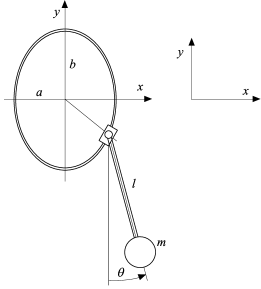
Figure 1: Schematic of an elliptically excited mechanical pendulum.

The extreme case of parametric excitation corresponds to $(e,\alpha)=(0,0)$. The other extreme case of horizontal excitation, which would be singular ($e\to\infty$) with our choice of parameters, has been studied theoretically in [34, 35].

The approximate expression (8) for the onset of rotations shows that the difference betwen both directions of rotation is most prominent if the parametric excitation is perturbed into an upright ellipse ($\alpha=\pi/2$ in (9)). Thus, we restrict our numerical study in section 4 to the specific model (1), which corresponds to $\alpha=\pi/2$. This gives rise to equation (1) for the elliptically excited pendulum as proposed in the introduction.

Figure 1 shows a mechanical representation of this model: a pendulum having mass $m$ and length $l$ is driven by a slider on an elliptic kinematic constraint. The slider is connected to the pendulum rod via a pin joint. The non-dimensional parameters and the non-dimensional time of model (1) can be obtained from the corresponding quantities of the mechanical representation by the scaling

$$\gamma =\frac{c}{\omega_{0}ml^{2}}\mbox{,} \omega =\frac{\Omega}{\omega_{0}}\mbox{,} t_{\mathrm{scaled}} =\omega_{0}\,t_{\mathrm{physical}}\mbox{,}$$ (10)

$$\omega_{0} =\sqrt{\frac{g}{l}}\mbox{,} p =\frac{a\Omega^{2}}{g}\mbox{,} ep =\frac{b\Omega^{2}}{g}\mbox{.}$$

In (10) $a$ is the amplitude of the vertical displacement excitation $a\cos(\Omega t)$, $b$ is the amplitude of the horizontal displacement excitation $b\sin(\Omega t)$, $\Omega$ is the driving frequency, $g$ is the acceleration due to gravity, $\omega_{0}$ is the linear natural frequency of the pendulum at the hanging-down angle $\theta=0$, $l$ is the length of the (mass-less) pendulor arm, $m$ is the mass of the pendulum bob, and $c$ is the viscous damping coefficient in the mechanical representation shown in figure 1.

4 Resonance Structure

In this section we analyse how the introduction of a nonzero ellipticity $e$ changes the resonance structure by constructing two-parameter bifurcation diagrams in the $\left(\omega,p\right)$-plane. We also use cross-sections of these diagrams (one-parameter bifurcation diagrams) at constant frequencies $\omega$ to make the connection between the different dynamical regimes visible. Throughout our study the bifurcation parameters are the excitation frequency $\omega$, the excitation amplitude $p$ and the ellipticity $e$ of the excitation. The parameter $e$ perturbs the reflection symmetry of the parametrically driven pendulum in the following way: if $(\theta(t),\dot{\theta}(t))$ is a solution for $e$ then $(-\theta(t),-\dot{\theta}(t))$ is a solution for $-e$. Thus, for any ellipticity $e$ the bifurcations obtained for $e$ are identical to those obtained for $-e$. This implies that we can restrict our attention to $e\geq 0$.

We slice the three-dimensional $(\omega,p,e)$-space along three two-dimensional planes by constructing three two-parameter bifurcation diagrams in the $(\omega,p)$-plane for three different values of $e$: $e=0$, $e=0.1$ and $e=0.5$. The case $e=0$ is the classical parametrically driven pendulum as studied in [12, 21, 15]. The case $e=0.1$ shows how a small perturbation of the reflection symmetry affects the classical bifurcation scenario and $e=0.5$ provides a picture of how the bifurcation scenario changes as the system deviates further from the parametric pendulum case towards a circular excitation.

The only remaining parameter in the non-dimensionalized equation (1) is the dimensionless viscous damping $\gamma$. We choose $\gamma=0.1$ to make our results comparable with the results of the previous studies [12, 21, 15].

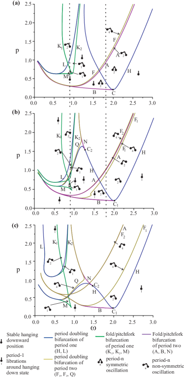
Figure 2: (colour online) Bifurcation diagrams in the $(\omega,p)$-plane for (a) $e=0$, (b) $e=0.1$, (c) $e=0.5$, computed with (R)AUTO [36, 37]. The figure 4 shows the one-parameter bifurcation diagrams along the dashed lines in (a) and (b) for $\omega=0.87$ and $\omega=1.8$, respectively. The damping $\gamma$ is $0.1$.

In the following we will discuss the bifurcations of oscillations and rotations separately. Oscillations are periodic orbits that stay in the potential well of the undriven conservative pendulum around the hanging-down position $\theta=0$. The average of the angular velocity over one period of an oscillation is zero. Rotations leave this potential well and have a non-zero average angular velocity along one period (for period-one rotations the average angular velocity is $\pm\omega$). We will present rotations and oscillations always in separate figures because they coexist over large parameter ranges and there is no local bifurcation linking the two types of periodic orbits.

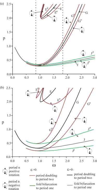
Figure 3: (colour online) Bifurcation diagrams in the $(\omega,p)$-plane comparing the bifurcations of the period-one rotations for $e=0.1$ (panel(a)) and $e=0.5$ (panel (b)) with the classical case $e=0$, computed with (R)AUTO [36, 37]. The figure 4 shows the one-parameter bifurcation diagrams along the dashed lines in (a) for $\omega=0.87$ and $\omega=1.8$, respectively. The damping $\gamma$ is $0.1$.

4.1 Overview of oscillations in the ($\omega$,p) plane

Figure 2 shows the two-parameter bifurcation diagrams in the $(\omega,p)$-plane for oscillations. Panel (a) shows the classical diagram for $e=0$, panel (b) presents the diagram for $e=0.1$, and panel (c) presents the diagram for $e=0.5$. The symbols between bifurcation curves in figure 2 indicate which attractors are observable in the different regions. The most prominent features of the classical diagram 2(a) are the two main resonance tongues where the hanging-down position $\theta=0$ loses its stability: the 1:2 resonance at $\omega\approx 2$ and the 1:1 resonance at $\omega\approx 1$. The 1:2 resonance tongue is bounded by the blue period-doubling curve H, and the 1:1 resonance tongue, which starts at a larger value of forcing ($p\approx 0.7$), is bounded by a pitchfork bifurcation curve (light green curves K_1,2 in figure 2(a)). Both tongues are separated by a region of stability of $\theta=0$ between the curves K₂ and H in figure 2(a). The period doubling H bounding the 1:2 resonance has a degeneracy at the point C: it is supercritical to the right of C and subcritical to the left of C.

The most significant change for nonzero ellipticity $e$ is that the two resonance tongues merge into a single region of instability. The period-doubling curve H merges with one of the non-symmetric period doubling curves L of the 1:1 tongue. This period doubling (still called H in figures 2(b) and 2(c)) and the fold curve K₁ form the stability boundary for the small-amplitude libration of period one around $\theta=0$, which is a perturbation of order $e$ of the hanging-down equilibrium position $\theta=0$ of the classical parametrically driven pendulum ($e=0$). The period doubling is subcritical between the points C₁ and C₂ along the curve H.

The one-parameter bifurcation diagrams along the parameter paths marked as dashed lines in figure 2(a) and (b) are discussed in detail in section 4.3. They show how the other bifurcation curves in figure 2 form the stability boundaries for the more complex oscillations. The values $\omega=1.8$ and $\omega=0.87$ for these parameter paths are representative for the 1:2 and the 1:1 resonance, respectively. They are the same as in [21], which studied the parametric case $e=0$.

4.2 Overview of rotations in the ($\omega$,p) plane

Figure 3 shows the bifurcations of period-one rotations for $e=0.1$ (figure 3(a)) and $e=0.5$ (figure 3(b)). The bifurcations of rotations in the parametric case $e=0$ are included (J and G, in black and grey) in both panels to show the effect of the nonzero ellipticity $e$. In all cases the stable period-one rotations are born, for increasing forcing $p$, in a fold bifurcation (curves J, J^p and Jⁿ in figure 3) and lose their stability in a period doubling bifurcation (curves G, G^p and Gⁿ in figure 3) as $p$ increases further. For even higher forcing the period-one rotation regains its stability (in the period doublings E, E^p and Eⁿ).

The most notable effect of the nonzero ellipticity is that all bifurcations are shifted toward lower forcing for rotations in the negative direction (that is, in the same rotiational sense as the motion of the base along the ellipse). The bifurcations of rotations in the positive direction are shifted upward. Approximation (8) estimates this effect in the limit of high frequency.

According to figure 1 the rotation in the negative direction ($\dot{\theta}<0$) rotates in the same direction as the base of the pendulum, corresponding to $\alpha=-\pi/2$ in (8). Thus, for $e>0$ the curve Jⁿ is shifted downwards from J by $2\gamma\omega e/(1+e)$ and the curve J^p is shifted upwards from J by $2\gamma\omega e/(1-e)$ in the limit $\omega\to\infty$. The equilibria of the averaged equation (6) show that negative rotations ($\alpha=-\pi/2$) pick up energy from the horizontal component of the forcing on average (that is, the factor in front of $\sin\phi$ is larger than one) whereas the positive rotations lose energy.

4.3 One-parameter diagrams for varying forcing amplitude

Figure 4 shows a series of four one-parameter bifurcation diagrams for varying forcing amplitude $p$. We pick two values for the frequency (the same as in [21]): $\omega=1.8$ (panel (a) and (b)), which is in the 1:2 resonance tongue, and $\omega=0.87$ (panel (c) and (d)), which is in the 1:1 resonance tongue, and two values for the ellipticity: $e=0$ (panel (a) and (c)) and $e=0.1$ (panel (b) and (d)). The vertical axis of all panels shows the coordinate $\theta$ of the stroboscopic map of (1) taken at $t=2k\pi/\omega$ where $k$ is a large integer. Stable oscillations and rotations are dark green thick lines, unstable oscillations and rotations are bright red thin lines. All bifurcation curves in the two-parameter diagrams figure 2 and figure 3 have been constructed by continuing the bifurcations shown as dark circles in figure 4. We have shifted the value of $\theta$ by $2\pi$ for all rotations to prevent curves associated with rotations and oscillations obscuring one another. The underlying black dots show the long-time behavior from the initial conditions $(\theta_{0},\dot{\theta}_{0})=(0.01\pi,0)$ (and $(\theta_{0},\dot{\theta}_{0})=(2\pi+0.01\pi,0)$) after waiting for a transient of 1000 periods of excitation, computed with Dynamics [38].

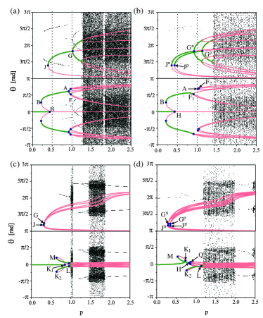
Figure 4: (colour online) One parameter bifurcation diagrams for the stroboscopic map of (1) for different values of $\omega$, varying the scaled forcing amplitude $p$ as the bifurcation parameter. The other parameters are $e=0$, $\omega=1.8$ in panel (a), $e=0.1$, $\omega=1.8$ in panel (b), $e=0$, $\omega=0.87$ in panel (c), and $e=0.1$, $\omega=0.87$ in panel (d). Black dots are the attractors computed for the initial condition $\theta_{0}=0.01\pi$, $\dot{\theta}_{0}=0$ with Dynamics [38]. The stable (thick dark green) and unstable (thin light red) periodic orbits, computed with (R)AUTO [36, 37], are superimposed. Oscillations are shown in the $\theta$-range of $[-\pi,\pi]$, rotations are shown in the $\theta$-range $[\pi,3\pi]$. The damping $\gamma$ is $0.1$. The basins of attraction shown in figure 5 have been computed at $p=0.5$, $p=1$, $p=1.4$ (see vertical dashed lines in panel (a) and (b)).

The main feature of the transition from $e=0$ to nonzero $e$ is the perturbation of the reflection symmetry. The symmetric system (with $e=0$) has the pitchfork bifurcations A (for period two in Figure 4(a)) and K₁ (for period one in Figure 4(c)) linking families of symmetric and nonsymmetric oscillations. These pitchfork bifurcations are perturbed into fold bifurcations (also named A and K₁ in the figures 4(b) and (d)).

The rotations (which are nonsymmetric orbits) and the nonsymmetric oscillations come in pairs of orbits symmetric to each other and lying on top of each other for $e=0$ in figures 4(a) and (c). The same applies to the bifurcations of the nonsymmetric orbits: the fold J and the period doubling G of the rotations, and the period doublings F and L for the nonsymmetric oscillations (starting rapidly accumulating period doubling cascades) are symmetric pairs of bifurcations, occuring simultaneously. This symmetry is broken by the increase of $e$ such that the formerly symmetric branches are now different: rotations in the negative direction emerging from the fold Jⁿ already exist for smaller forcing $p$ than the rotations in the positive direction emerging from J^p, which are shifted toward larger forcing $p$. Similarly, the formerly symmetric pairs of nonsymmetric oscillations lose their symmetry: one family is always shifted toward larger $p$ (born at the fold F₂ in Figure 4 (b), and K₂ in Figure 4 (d)), the other family becomes a continuous extension of the formerly symmetric oscillation.

For $\omega=1.8$ the visibility of chaotic attractors (bands of small black dots in figure 4) is shifted toward larger $p$ by the symmetry breaking because stable periodic rotations exist for larger $p$ (up to $p\approx 1.35$). At $\omega=0.87$ the simulation also showed period-two oscillations jumping between two potential wells for larger $p$ in the simulation results (black lines evident after the chaotic bands in panels (c) and (d)).

Figure 5 shows how the basins of attraction lose their symmetry when one increases $e$ from $0$ to $0.1$. The colour coding of each point in the $(\theta,\dot{\theta})$-plane is chosen according to the attractor which the stroboscopic map reaches starting from this point.

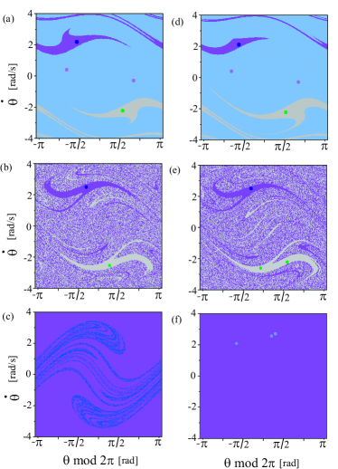
Figure 5: (colour online) Basins of attraction for different values of the forcing amplitude, $p$, and ellipticity $e$, computed with Dynamics [38]. Panel (a): $e=0$, $p=0.5$, (b): $e=0$, $p=1$, (c): $e=0$, $p=1.4$, (d): $e=0.1$, $p=0.5$, (e): $e=0.1$, $p=1$, (f) $e=0$, $p=1.4$. The other parameters are $\gamma=0.1$ and $\omega=1.8$. Stable periodic orbits are shown as large dots (their colour is chosen to give a contrast to their own basin of attraction).

The forcing is $p=0.5$ in figure 5 (a) and (d), $p=1$ in panels (b) and (e), and $p=1.4$ in panels (c) and (f). The periodic attractors (shown as dots) with $\dot{\theta}$-coordinates $\approx\pm 2$ correspond to periodic rotations. The panels (d) and (e) show that for small $p$ ($p=0.5$ and $p=1$) one direction of rotation (negative) has a visibly larger basin of attraction than the other. At $p=1.4$ the change of $e$ caused a crisis of the chaotic attractor in panel (c), creating a period-three rotation.

For further increase of $e$ the effect that one attractor of the formerly symmetric pair of nonsymmetric periodic orbits is shifted toward higher values of forcing becomes more pronounced (as shown in the the two-parameter diagrams in figure 2(c) and figure 3(b)). This shift depends strongly and nonlinearly on $e$: for example, formula (8) already underestimates this shift for J^p by 20% for $e=0.5$, which still corresponds to a narrow ellipse.

5 Conclusions

Introducing a horizontal component into the excitation of the classical parametrically excited pendulum results in a symmetry breaking scenario. The excitation changes from a purely vertical motion to a motion on an ellipse. The main effects of this ellipticity are twofold: first, the well-known 1:2 and 1:1 resonance tongues of the classical parametric pendulum merge into a single region of instability, bounded by a period doubling and a fold (saddle-node) bifurcation of the small amplitude oscillation. Second, rotations of the pendulum that have the same direction as the base motion pick up energy from the horizontal excitation such that they are present at lower overall forcing amplitudes. For example, clockwise motion of the pivot around the ellipse results in a preference for clockwise rotations of the pendulum.

Both effects of ellipticity are favorable for rotation: the first effect implies that small-amplitude oscillations around the hanging-down position, which are attractors competing with rotations, lose their stability for smaller forcing compared with the $e=0$ case. The second effect means that the parameter region in the frequency-amplitude plane where rotations are supported increases with increasing ellipticity. The excitation amplitude necessary to sustain rotations in both directions also increases with increasing $e$ because of the increasing ‘imperfection’ of the symmetry.

A comparison between the bifurcation scenarios of the model and an actual experiment is still outstanding. Direct bifurcation analysis for experiments is a challenging task that may require the development of entirely new experimental methods. Apart from this lack of experimental verification, other open questions are: the high-frequency approximation (8) suggests that for a circular excitation ($e=1$, $\alpha=\pi/4$) rotations against the base excitation are impossible regardless of the level of forcing and damping. This is not true in general for lower frequency and sufficiently small damping. Thus, we expect that, depending on the shape of the excitation, there must be a critical damping level below which rotations against the excitation direction become possible for a suitable range of the excitation amplitudes and frequencies.

The small dissipation restricts the type of bifurcations and regimes encountered in the system (for example, torus bifurcations are impossible). We expect that even a small amount of interaction between the pendulum and the base ([11]) will lead to large regions in the frequency-forcing plane where one can observe quasi-periodicity. Escape from a potential well tends to lead to indeterminacy as introduced in [39]. The precise sequence of heteroclinic tangencies leading to escape from the potential well is still largely unknown even for the parametrically excited pendulum.

References

- [1] R. W. Leven, B. P. Koch, Chaotic behaviour of a parametrically excited damped pendulum, Physics Letters 86A (2) (1981) 71–74.
- [2] E. I. Butikov, The rigid pendulum - an antique but evergreen physical model, European Journal of Physics 20 (6) (1999) 429–441.
- [3] A. Mouchet, C. Eltschka, P. Schlagheck, Influence of classic resonances on chaotic tunneling, Physical Review E 74 (2006) 026211–11.
- [4] W. C. Stewart, Current-voltage characteristics of josephson junctions, Applied Physics Letters 12 (8) (1968) 277–280.
- [5] G. L. Baker, J. A. Blackburn, H. J. T. Smith, The quantum pendulum: small and large, American Journal of Physics 70 (2002) 525–531.
- [6] J. L. Trueba, J. P. Baltanás, M. A. F. Sanjuán, A generalized perturbed pendulum, Chaos, Solitons and Fractals 15 (5) (2003) 911–924.
- [7] H. J. T. Smith, J. A. Blackburn, Experimental study of an inverted pendulum, American Journal of Physics 60 (1992) 909–911.
- [8] J. A. Blackburn, G. L. Baker, A comparison of commercial chaotic pendulums, American Journal of Physics 66 (1998) 821–830.
- [9] S. Y. Kim, S. H. Shin, J. Yi, C. W. Jang, Bifurcations in a parametrically forced magnetic pendulum, Physical Review E 56 (1997) 6613–6619.
- [10] B. Horton, M. Wiercigroch, X. Xu, Transient tumbling chaos and damping identification for parametric pendulum, Philosophical Transactions of the Royal Society of London, A 366 (2007) 767–784.
- [11] X. Xu, E. Pavlovskaia, M. Wiercigroch, F. Romeo, and S. Lenci. Dynamic interac- tions between parametric pendulum and electro-dynamical shaker. ZAMM 82 (2) (2007) 172–186.
- [12] W. Szemplińska-Stupnicka, E. Tyrkiel, Common features of the onset of the persistent chaos in nonlinear oscillators: A phenomenological approach, Nonlinear Dynamics 27 (3) (2002) 271–293.
- [13] P. J. Bryant, J. W. Miles, On a periodically forced, weakly damped pendulum. part 3: vertical forcing, Journal of the Australian Mathematical Society, Series B 32 (1990) 42–60.
- [14] M. J. Clifford, S. R. Bishop, Locating oscillatory orbits of the parametrically-excited pendulum, Journal of the Australian Mathematical Society, Series B 37 (1996) 309–319.
- [15] X. Xu, M. Wiercigroch, Approximate analytical solutions for oscillatory and rotational motion of a parametric pendulum, Nonlinear Dynamics 47 (2007) 311–320.
- [16] S. Lenci, E. Pavlovskaia, G. Rega, M. Wiercigroch, Rotating solutions and stability of parametric pendulum by perturbation method, Journal of Sound and Vibration 310 (1-2) (2008) 243–259.
- [17] J. Isohätälä, K. N. Alekseev, L. T. Kurki, P. Pietiläinen, Symmetry breaking in a driven and strongly damped pendulum, Physical Review E 71 (2005) 066206–6.
- [18] S. R. Bishop, M. J. Clifford, The use of manifold tangencies to predict orbits, bifurcations and estimate escape in driven systems, Chaos, Solitons and Fractals 7 (10) (1996) 1537–1553.
- [19] M. J. Clifford, S. R. Bishop, Approximating the escape zone for the parametrically excited pendulum, Journal of Sound and Vibration 172 (4) (1994) 572–576.
- [20] I. W. Stewart, T. R. Faulkner, Estimating the escape zone for a parametrically excited pendulum-type equation, Physical Review E 62 (2000) 4856–4861.
- [21] X. Xu, M. Wiercigroch, M. P. Cartmell, Rotating orbits of a parametrically-excited pendulum, Chaos, Solitons and Fractals 23 (5) (2005) 1537–1548.
- [22] D. Capecchi, S. R. Bishop, Periodic oscillations and attracting basins for a parametrically excited pendulum, Dynamics and Stability of Systems 9 (2) (1994) 123–143.
- [23] H. J. T. Smith, J. A. Blackburn, Multiperiodic orbits in a pendulum with a vertically oscillating pivot, Physical Review E 50 (1994) 539–549.
- [24] W. Szemplińska-Stupnicka, E. Tyrkiel, A. Zubrzycki, The global bifurcations that lead to transient tumbling chaos in a parametrically driven pendulum, International Journal of Bifurcation and Chaos 10 (9) (2000) 2161–2175.
- [25] R. Kobes, J. Lui, S. Pele, Analysis of a parametrically driven pendulum, Physical Review E 63 (2000) 036219–17.
- [26] S. Y. Kim, K. Lee, Multiple transitions to chaos in a damped parametrically forced pendulum, Physical Review E 53 (1995) 1579–1586.
- [27] S. R. Bishop, A. Sofroniou, P. Shi, Symmetry-breaking in the response of the parametrically excited pendulum model, Chaos, Solitons and Fractals 25 (2) (2005) 257–264.
- [28] P. Hagedorn, J. Wallaschek, Travelling wave ultrasonic motors, Part I: Working principle and mathematical modelling of the stator, Journal of Sound and Vibration 155 (1) (1992) 31–46.
- [29] N. W. Hagood IV, A. J. McFarland, Modeling of a piezoelectric rotary ultrasonic motor, IEEE Transactions on Ultrasonics, Ferroelectrics and Frequency Control 42 (2) (1995) 210–224.
- [30] E. Ott, C. Grebogi, J. Yorke, Controlling chaos, Phys. Rev. Lett. 64 (1990) 1196–1199.
- [31] K. Pyragas, Continuous control of chaos by self-controlling feedback, Physics Letters A 170 (1992) 421–428.
- [32] W. van de Water, J. de Weger, Failure of chaos control, Phys. Rev. E 62 (5) (2000) 6398–6408.
- [33] A. Fidlin, J. T. Thomsen, Non-trivial effects of high-frequency excitation for strongly damped mechanical systems, Int. J. Nonlinear Mechanics 43 (2008) 569–578.
- [34] R. V. Dooren, Chaos in a pendulum with forced horizontal support motion: a tutorial, Chaos, Solitons and Fractals 7 (1996) 77–90.
- [35] O. V. Kholostova, Some problems of the motion of a pendulum when there are horizontal vibrations of the point of suspension, Journal of Applied Mathematics and Mechanics 59 (1995) 553–561.
- [36] E. J. Doedel, T. F. Fairgrieve, B. Sandstede, X. Wang, Y. A. Kuznetsov, A. R. Champneys, Auto 97: Continuation and bifurcation software for ordinary differential equations (1998).
- [37] F. Schilder, RAUTO: running AUTO more efficiently, http://www.dynamicalsystems.org/sw/sw/ (2007).
- [38] H. E. Nusse, J. A. Yorke, Dynamics: Numerical explorations, volume 101 of Applied Mathematical Sciences. Springer-Verlag New York, Inc., second, revised and enlarged edition, 1998.
- [39] J. M. T. Thompson, Chaotic phenomena triggering the escape from a potential well, Proc. Roy. Soc. Lond. A 421 (1862) (1989) 195–225.