On an excitation mechanism for trapped inertial waves in discs around black holes

Abstract

According to one model, high-frequency quasi-periodic oscillations (QPOs) can be identified with inertial waves, trapped in the inner regions of accretion discs around black holes due to relativistic effects. In order to be detected, their amplitudes need to reach large enough values via some excitation mechanism. We work out in detail a non-linear coupling mechanism suggested by Kato, in which a global warping or eccentricity of the disc has a fundamental role. These large-scale deformations combine with trapped modes to generate ‘intermediate’ waves of negative energy that are damped as they approach either their corotation resonance or the inner edge of the disc, resulting in amplification of the trapped waves. We determine the growth rates of the inertial modes, as well as their dependence on the spin of the black hole and the properties of the disc. Our results indicate that this coupling mechanism can provide an efficient excitation of trapped inertial waves, provided the global deformations reach the inner part of the disc with non-negligible amplitude.

1 Introduction

In the past two decades, and mainly thanks to NASA’s Rossi X-ray Timing Explorer (RXTE), about $20$ X-ray binaries, believed to contain a black hole, have been analysed in detail (Remillard & McClintock, 2006a). An important characteristic of these objects is rapid X-ray variability (van der Klis, 2006), in which quasi-periodic oscillations (QPOs) are included. Of particular relevance are high-frequency quasi-periodic oscillations (HFQPOs), features observed in the power spectra of the light curves of black hole candidates, which are a potentially important tool in the study of strong gravitational fields. The frequencies observed, and their stability against luminosity variations, suggest a connection with the inner accretion flow (Remillard & McClintock, 2006b). Some authors (Nowak et al., 1997; Wagoner, 1999; Nowak & Lehr, 1999; Kato, 2001) argued that these oscillations can be explained in terms of modes arising in the accretion disc that surrounds the black hole. Turbulent viscosity, characteristic of accretion flows, generally prevents waves from propagating across the disc to form coherent global modes. A possible way for such modes to exist is for them to be trapped in a small region in the inner part of the disc. Radial trapping of waves was first predicted by Kato & Fukue (1980), who considered oscillations in a disc around a Schwarzschild black hole, and was studied further by Okazaki et al. (1987). Although trapped waves may reveal relatively little about the properties of the accretion disc itself, they are a promising tool in the study of the central object. According to Remillard & McClintock (2006b), a good model of HFQPOs would provide the most reliable avenue for measuring black hole spins. Once their masses are also determined, an important step in testing the Kerr metric will be taken.

For trapped oscillations to explain HFQPOs, an excitation mechanism for these modes is required, as their amplitudes need to reach values high enough to allow detection. A possibility can reside in the interaction between waves in the disc and a global deformation (warping or eccentricity). Goodman (1993) initially studied the local excitation of waves in a tidally distorted disc via the parametric instability. The idea of using a warp as an excitation mechanism for disc oscillations goes back to Papaloizou & Terquem (1995), who mentioned the possibility of parametric generation of inertial waves. Detailed calculations are reported by Gammie et al. (2000). More recently, and using a different approach, this problem was studied analytically for thin, relativistic discs with non-rotating central objects by Kato (2004) (see also Kato (2007), where similar calculations are made for eccentric discs). He made simple estimates for the growth rates of trapped inertial modes, which are of considerable interest. On the other hand, there are many uncertainties in his calculations and he did not discuss the origin or nature of the global deformations.

In this paper we develop and generalize Kato’s ideas on this excitation mechanism and make detailed numerical calculations of the modes and growth rates for rotating black holes. We include a dynamical treatment of the warp or eccentricity but defer to a second paper a broader discussion of the origin and global propagation of these deformations.

In Section 2 we review the trapping of inertial oscillations in a simple, pseudo-relativistic disc model. In Section 3 we describe the excitation mechanism for trapped inertial modes, which relies on a coupling between waves in the disc and global deformations. In Section 4 we discuss the dependence of the inertial modes’ growth rates on disc parameters and black hole spin. Conclusions are presented in Section 5.

2 Trapped inertial oscillations

2.1 Basic equations

The trapping of oscillations can be easily understood by analysing the fluid equations in a simple isothermal disc model (Lubow & Pringle, 1993; Kato, 2001). Although this trapping happens only in discs around compact objects, a fully relativistic model is not necessary. The most important effects can be included by supplementing a Newtonian treatment with the correct relativistic expressions for the characteristic frequencies in the disc (Kato, 2001). For simplicity and clarity, we adopt this pseudo-relativistic approach and consider a strictly isothermal disc with a ratio of specific heats $\gamma=1$. Ignoring viscosity and magnetic fields, the fundamental hydrodynamic equations can be written as

$$\frac{\partial\mn@boldsymbol{u}}{\partial t}+\mn@boldsymbol{u}\cdot\nabla\mn@boldsymbol{u}=-\nabla{h}-\nabla\Phi,$$ (1)

$$\frac{\partial h}{\partial t}+\mn@boldsymbol{u}\cdot\nabla h=-c_{\mathrm{s}}^{2}\nabla\cdot\mn@boldsymbol{u},$$ (2)

where $h=c_{\mathrm{s}}^{2}\log\rho$ is the enthalpy and $c_{\mathrm{s}}$ is the constant sound speed in the disc. We neglect self-gravitation and consider a fixed axisymmetric gravitational potential $\Phi(r,z)$, where $(r,\phi,z)$ are cylindrical polar coordinates.

2.2 Linearized equations

As in the case of stars (Christensen-Dalsgaard, 2002), to study oscillations one needs to analyse what happens to this system of equations when the velocity and enthalpy are perturbed: $q=q_{0}+q^{\prime}$. The equilibrium state of the disc is independent of time and azimuth: $\mn@boldsymbol{u}_{0}=\mn@boldsymbol{\Omega}\times\mn@boldsymbol{r}=r\Omega(r)\mn@boldsymbol{e}_{\phi}$, where $\Omega$ is the angular velocity, which is independent of $z$ in a strictly isothermal disc, while $h_{0}(r,z)$ satisfies $\mn@boldsymbol{\nabla}h_{0}=r\Omega^{2}\mn@boldsymbol{e}_{r}-\mn@boldsymbol{\nabla}\Phi$. Thus the perturbations acting on it can be written as

$$q^{\prime}(r,\phi,z,t)=\textrm{Re}\left[\widetilde{q^{\prime}}(r,z)\exp(\textrm{i}m\phi-\textrm{i}\omega t)\right],$$ (3)

where $m$ is the azimuthal mode number and $\omega$ is the oscillation frequency. Dropping, for simplification, the tildes and zeros, the linearized equations for the perturbed quantities can be written in the form

$$-\mathrm{i}\hat{\omega}u^{\prime}_{r}-2\Omega u^{\prime}_{\phi}=-\frac{\partial h^{\prime}}{\partial r},$$ (4)

$$-\mathrm{i}\hat{\omega}u^{\prime}_{\phi}+\frac{\kappa^{2}}{2\Omega}u^{\prime}_{r}=-\frac{\textrm{i}mh^{\prime}}{r},$$ (5)

$$-\mathrm{i}\hat{\omega}u^{\prime}_{z}=-\frac{\partial h^{\prime}}{\partial z},$$ (6)

$$-\mathrm{i}\hat{\omega}h^{\prime}-\Omega_{z}^{2}zu^{\prime}_{z}=-c_{\mathrm{s}}^{2}\left[\frac{1}{r}\frac{\partial(ru^{\prime}_{r})}{\partial r}+\frac{\textrm{i}mu^{\prime}_{\phi}}{r}+\frac{\partial u^{\prime}_{z}}{\partial z}\right],$$ (7)

where $\hat{\omega}=\omega-m\Omega$ is the Doppler-shifted wave frequency, which is zero at the corotation radius, and $\kappa$ and $\Omega_{z}$ are the epicyclic and vertical frequencies, respectively (Binney & Tremaine, 1988). We apply the thin disc approximation ($\partial h/\partial z=-\Omega_{z}^{2}z$), and neglect the term $u^{\prime}_{r}\partial h/\partial r$ in the last equation. The latter approximation is valid if the radial wavelength for perturbations is smaller than the radial scale on which the enthalpy varies in the basic state. Variables can then be further separated in $r$ and $z$, using (Okazaki et al., 1987)

$$(u^{\prime}_{r},u^{\prime}_{\phi},h^{\prime})=\left(u_{r}(r),u_{\phi}(r),h(r)\right)\textrm{He}_{n}\left(\frac{z}{H}\right),$$ (8)

$$u^{\prime}_{z}=u_{z}(r)\textrm{He}_{n-1}\left(\frac{z}{H}\right),$$ (9)

where $\textrm{He}_{n}$ is the modified Hermite polynomial of order $n$ (Abramowitz & Stegun, 1972), with $n=0,1,2,3,\dots$ being the vertical mode number and $H=\sqrt{c_{\mathrm{s}}/\Omega_{z}}$ the vertical scaleheight of the disc. (Since $\textrm{He}_{-1}$ is not defined, for $n=0$ we have $u^{\prime}_{z}=0$.) It should be noted that this separation of variables is not exact since $H$ depends on $r$ (as described by Kato (2001), this separation is valid to lowest WKB order; Nowak & Wagoner (1992) use a slowly varying function of $r$ to separate variables). The variation of $H$ with $r$ couples different vertical modes (Tanaka et al., 2002) but this effect is weak when the radial wavelength is short, and we neglect it. The final set of ordinary differential equations in $r$ for the perturbed quantities reads

$$-\mathrm{i}\hat{\omega}u_{r}-2\Omega u_{\phi}=-\frac{\mathrm{d}h}{\mathrm{d}r},$$ (10)

$$-\mathrm{i}\hat{\omega}u_{\phi}+\frac{\kappa^{2}}{2\Omega}u_{r}=-\frac{\mathrm{i}mh}{r},$$ (11)

$$-\mathrm{i}\hat{\omega}u_{z}=-n\frac{h}{H},$$ (12)

$$-\mathrm{i}\hat{\omega}h-\Omega_{z}^{2}Hu_{z}=-c_{\mathrm{s}}^{2}\left[\frac{1}{r}\frac{\mathrm{d}(ru_{r})}{\mathrm{d}r}+\frac{\mathrm{i}mu_{\phi}}{r}\right].$$ (13)

2.3 Wave modes

The dispersion relation for wave modes in the disc can be determined by further assuming that the radial wavelength of the perturbed quantities is much smaller than both the azimuthal wavelength and the characteristic scale for radial variations of the equilibrium quantities. It can then be verified that perturbations with local radial wavenumber $k$ obey (Okazaki et al., 1987)

$$k^{2}=\frac{(\hat{\omega}^{2}-\kappa^{2})(\hat{\omega}^{2}-n\Omega_{z}^{2})}{\hat{\omega}^{2}c_{\mathrm{s}}^{2}}.$$ (14)

As argued before, the most important relativistic effects on wave propagation can be included by using relativistic expressions for the characteristic frequencies. For a particle orbit, these read (Kato, 1990),

$$\Omega=(r^{3/2}+a)^{-1},$$ (15)

$$\kappa=\Omega\sqrt{1-\frac{6}{r}+\frac{8a}{r^{3/2}}-\frac{3a^{2}}{r^{2}}},$$ (16)

$$\Omega_{z}=\Omega\sqrt{1-\frac{4a}{r^{3/2}}+\frac{3a^{2}}{r^{2}}},$$ (17)

where $a$ is the dimensionless spin parameter of the central object ($-1<a<1$), $r$ is in units of the gravitational radius $r_{\textrm{g}}=GM/c^{2}$ and the frequencies are in units of $c^{3}/GM$, where $c$ is the speed of light, $G$ the gravitational constant and $M$ the mass of the black hole. We assume that the characteristic frequencies in the disc can be approximated by these particle orbit expressions. Of great importance is the variation of the epicyclic frequency $\kappa$ with $r$: as $r$ decreases, $\kappa$ increases, reaches a maximum and then goes to zero at the radius of the marginally stable orbit, $r_{\rm ms}$, which can be regarded as the inner edge of the accretion disc. Since we are interested in studying oscillations in accretion discs around compact objects, we adopt these relativistic expressions. They correctly describe the frequency and stability of orbits in the Kerr metric, as well as the apsidal and nodal precession rates, but some information about the metric coefficients is lost in this pseudo-relativistic approach.

From the dispersion relation we can see that, if $n\neq 0$, two types of wave-like solutions, propagating in different regions in the disc, are possible: a high-frequency one with $\hat{\omega}^{2}>\textrm{max}(\kappa^{2},n\Omega_{z}^{2})=n\Omega_{z}^{2}$ (p mode) and a low-frequency one with $\hat{\omega}^{2}<\textrm{min}(\kappa^{2},n\Omega_{z}^{2})=\kappa^{2}$ (r mode). If $n=0$ the dispersion relation for the non-trivial mode becomes $\hat{\omega}^{2}=k^{2}c_{\mathrm{s}}^{2}+\kappa^{2}$ and waves can propagate where $\hat{\omega}^{2}>\kappa^{2}$; this is the inertial-acoustic mode. In non-isothermal discs the closest equivalent of this mode behaves like a surface gravity wave or stellar f mode (Ogilvie, 1998; Lubow & Ogilvie, 1998) but here we refer to it as the $n=0$ mode or 2D mode, since it involves a purely horizontal motion independent of $z$.

The inertial or r modes (so called by Korycansky & Pringle, 1995) are nearly incompressible since they are restored by inertial forces, avoiding acoustic effects. (They are often called g modes in the literature, but they are not related to internal gravity waves or stellar g modes.) Acoustic or p modes have pressure as their main restoring force and are essentially compressible. In an isothermal disc, the 2D mode is a purely horizontal compressible mode.

The propagation regions of the p and r modes allow us to define important radii in the disc, the resonant radii (e.g. Lubow & Ogilvie, 1998). Non-axisymmetric waves can have three types of resonances: corotation where $\hat{\omega}=0$, Lindblad resonances where $\hat{\omega}^{2}-\kappa^{2}=0$, and vertical resonances where $\hat{\omega}^{2}-n\Omega_{z}^{2}=0$ (for $n\neq 0$). Lindblad resonances are turning points for the r and 2D modes, while vertical resonances are turning points for p modes.

The three different types of modes propagate in different regions in the disc. If the epicyclic frequency has a maximum at some particular radius, r and 2D modes can be trapped in the inner part of the disc, while p modes always propagate to the outer boundary beyond the outer vertical resonance. Originally Kato & Fukue (1980) considered the trapping of 2D modes in the very inner region of the disc. These modes can be trapped between the radius of the marginally stable orbit and the inner Lindblad resonance. However, the conditions at $r_{\mathrm{ms}}$ are not well understood and it is not clear if this trapping region can work as a resonant cavity. Therefore, here we focus on the trapping of r modes, which happens below the maximum of the epicyclic frequency between two Lindblad resonances (and with no corotation resonance in between), a resonant cavity naturally created by the non-monotonic variation of $\kappa$ with radius (Okazaki et al., 1987).

Of particular importance is the axisymmetric trapped wave with frequency $\omega\approx\textrm{max}(\kappa)$, and with the simplest possible radial structure. This mode is trapped in a small region close to the maximum of the epicyclic frequency, and is important, not only because it is naturally confined and therefore more likely to occur in the presence of turbulent viscosity, but also because its frequency can be identified with $\textrm{max}(\kappa)$, which depends only on the properties of the black hole: its mass $M$ and its angular momentum $a$. Furthermore, this mode is likely to be most easily observed, as it may produce a net luminosity variation of the disc without cancellations. Therefore, measuring the frequency of this mode and determining the mass of the central object by, e.g., studying the orbit of its binary companion, one can, in principle, find the spin of the black hole.

2.4 Numerical calculation of trapped r modes

To find the radial structure of trapped modes we need to solve the system of equations (10)–(13), subject to appropriate boundary conditions. Numerical calculations of waves trapped near the maximum of the epicyclic frequency were first performed by Okazaki et al. (1987). Here we focus on the simplest possible trapped inertial modes, with $m=0$ and $n=1$. An approximate analysis of equations (10)–(13) close to the maximum of the epicyclic frequency shows that, between the two Lindblad resonances, these solutions are described by parabolic cylinder functions (Abramowitz & Stegun, 1972) involving Hermite polynomials of order $l=0,1,2,\dots$, centred at the maximum of $\kappa$, like the solutions of the quantum harmonic oscillator (Perez et al., 1997). The lowest order mode ($l=0$) has a Gaussian structure in $r$. In this section we solve the same problem using numerical methods and fewer approximations, as a prelude to an analysis of the non-linear mode couplings that cause these modes to grow.

Since we expect to find trapped modes only for some discrete values of the oscillation frequency, we solve the set of equations as a generalized eigenvalue problem, of the form

$$\mathbf{A}\mn@boldsymbol{U}=-\textrm{i}\omega\mathbf{B}\mn@boldsymbol{U},$$ (18)

where $\mn@boldsymbol{U}$ is the column vector whose components are the r mode quantities $(u_{r},u_{\phi},u_{z},h)$ evaluated at a set of discrete points, $\mathbf{A}$ is the matrix representing the system of equations (10)–(13), and $\mathbf{B}$ can be different from the identity matrix depending on the boundary conditions used. To solve this problem numerically, we use a pseudo-spectral method with Chebyshev polynomials. We use a Gauss–Lobatto grid, $x(i)=\textrm{cos}(\pi i/N)$, where $N$ is the number of grid points, and the Chebyshev coordinate $-1<x<1$ is related to the radial coordinate by

$$r=-x\frac{r_{\mathrm{out}}-r_{\mathrm{in}}}{2}+\frac{r_{\mathrm{out}}+r_{\mathrm{in}}}{2},$$ (19)

so that $r_{\mathrm{in}}<r<r_{\mathrm{out}}$, where $r_{\mathrm{in}}=r_{\mathrm{ms}}$ and $r_{\mathrm{out}}$ is an outer radius chosen to be larger than the outer Lindblad resonance for the r mode. The representation of the first derivatives in the matrix $\mathbf{A}$ is achieved using the Chebyshev collocation derivative matrix, defined by (Boyd, 2001)

$$D_{ij}=\begin{cases}(1+2N^{2})/6&i=j=0\\ -(1+2N^{2})/6&i=j=N\\ -x_{j}/[2(1-x_{j}^{2})]&i=j,\,j\neq 0,N\\ (-1)^{i+j}p_{i}/[p_{j}(x_{i}-x_{j})]&i\neq j,\end{cases}$$ (20)

where $p_{0}=p_{N}=2$, and $p_{j}=1$ otherwise. The generalized eigenvalues and eigenfunctions of $\mathbf{A}$ are then calculated numerically, using IDL’s eigenvalue solver, LA_EIGENPROBLEM, which uses a QR decomposition, and is based on LAPACK routines. The boundary conditions used are the following:

• At $\mn@boldsymbol{r_{\mathrm{in}}}$    $u_{r}=0$. According to the dispersion relation, the r mode is expected to be exponentially decaying for radii smaller than its innermost Lindblad resonance and therefore its velocity is supposed to be approximately zero at the marginally stable orbit, which justifies the choice of this boundary condition.

• At $\mn@boldsymbol{r_{\mathrm{out}}}$    $\textrm{d}u_{r}/\textrm{d}r=\textrm{i}ku_{r}$, where $k$ is given by the dispersion relation (14) for $m=0$, $n=1$ at $r_{\mathrm{out}}$, and using $\omega\approx\textrm{max}(\kappa)$. Since the r mode can propagate again as a p mode outside the vertical resonance, we choose an outer radius beyond this location, so that the mode is oscillatory there, i.e., $k$ is real, and we select the outgoing wave solution by choosing $k>0$ so that the group velocity of the waves at $r_{\mathrm{out}}$ is positive. This condition allows the wave to lose energy through the outer boundary and minimizes artificial wave reflection there.

We allow for the possibility that $\omega$ is complex, in which case its imaginary part is the growth rate of the disturbance. In fact, in the absence of non-linear mode couplings, we obtain slowly decaying solutions with $\mathrm{Im}(\omega)<0$ as a result of the outgoing-wave outer boundary condition.

In Fig. 1 we show the variation of $u_{r}$ with radius for two typical trapped solutions, corresponding to two different radial mode numbers $l=0$ and $l=1$. (Since we are solving an eigenvalue problem, solutions are multiplied by an arbitrary amplitude.) The complex frequencies of the modes represented in Fig. 1 are $0.03196-3.6884\times 10^{-7}\textrm{i}$ and $0.02989-1.1846\times 10^{-7}\textrm{i}$ (in units of $c^{3}/GM$), respectively. In these units, and for the value of $a$ used, the maximum of $\kappa$ is 0.03312. These modes are slightly damped because of the boundary condition used at the outer radius, which selects the outgoing wave only. If the sound speed is smaller, the frequency of the modes is closer to the value of the epicyclic frequency at its maximum, and the trapping region and damping rate are smaller (see Tab. 1). We obtained identical results by solving the two-point boundary-value problem using a shooting method.

$c_{\mathrm{s}}/c$	frequency
$0.002$	$0.03289+0.0\textrm{i}$
$0.005$	$0.03254-1.276\times 10^{-10}\textrm{i}$
$0.01$	$0.03196-3.688\times 10^{-7}\textrm{i}$
$0.02$	$0.03079-2.417\times 10^{-5}\textrm{i}$

Table 1: Dependence of the real and imaginary part of the $l=0$ r mode frequency (in units of $c^{3}/GM$) on the sound speed $c_{\mathrm{s}}$, for $a=0.5$. We use 150 collocation points and a value of 18.2331 for the outer radius, in units of $GM/c^{2}$ ($r_{\mathrm{in}}=r_{\mathrm{ms}}=4.2331$).

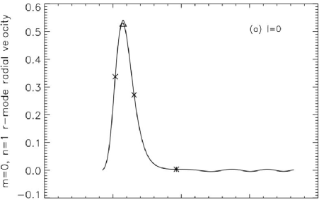
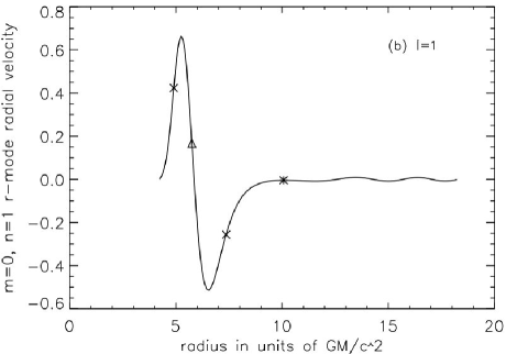
Figure 1: Variation of the real part of the radial component of the axisymmetric, $n=1$ r mode velocity with radius for $c_{\mathrm{s}}/c=0.01$ and $a=0.5$ for (a) $l=0$ and (b) $l=1$. The triangle indicates the radius where the epicyclic frequency is maximum, and the crosses and asterisks the Lindblad and vertical resonances, respectively.

These inertial modes can be thought of as waves trapped in a virtual potential, $U(r)=-k(r)^{2}$ (Li et al., 2003), which for a frequency close to the maximum of $\kappa$ is similar to the harmonic oscillator potential. If $U(r)<0$ waves can propagate, being evanescent in the regions where potential barriers exist. Also, as in quantum mechanics, these trapped inertial waves can escape through the potential barriers and propagate on the other side, as p modes. The inertial modes are evanescent between the inner radius and the first Lindblad resonance and between the second Lindblad resonance and the vertical one. The ‘leakage’ through the potential barrier is also verified, as our results show small-amplitude oscillations after the vertical resonance (Fig. 1). The larger the sound speed, the larger the width and smaller the height of the barrier, and more ‘leakage’ through the barrier is expected, which is verified numerically (Tab. 1). This ‘leakage’ was first predicted by Okazaki et al. (1987).

As described above, the inertial mode characterized by $(l,m,n)=(0,0,1)$ is likely to be relevant to the interpretation of observed oscillations. In the next section we describe an excitation mechanism for this mode, based on non-linear wave coupling. If the modes are not strongly coupled, we expect the mechanism to affect mainly the growth rate $\mathrm{Im}(\omega)$, so that the structure of the wave still resembles a Gaussian centred at the maximum of $\kappa$, as shown in Fig. 1 (a).

3 Growth of oscillations in deformed discs

Low-frequency modes with azimuthal mode number $m=1$ have been widely studied in the context of (quasi-)Keplerian accretion disc theory (Kato, 1983), since they are global, typically vary on length-scales comparable to the radial extent of the disc, and are long-lived. Kato (1989) showed that these modes are also global in a relativistic disc. A global $m=1$ mode with one node in the vertical direction ($n=1$) is typically identified with a warp in the disc (Papaloizou & Lin, 1995), while $n=0$ modes correspond to eccentric discs. This is easily seen if we focus on the action of each of these modes on a ring. The vertical displacement of a $m=1,n=1$ mode is independent of $z$, and proportional to $\cos(\phi-\textrm{constant})$ at fixed $r$ and $t$, which corresponds to a tilting, as the displacement with respect to the disc plane is different at each azimuthal angle. In the case of the $n=0$ mode, the radial displacement is the one that is independent of $z$, and proportional to $\cos(\phi-\textrm{constant})$ at fixed $r$ and $t$. This means that the displacement within the disc plane varies with $\phi$, creating an elliptical orbit. As we discuss below, these global deformation modes can be produced by the presence of a binary companion or by instabilities.

3.1 Warped discs

It is believed that warps exist in many astrophysical discs. Precessing warped discs have been used successfully to explain long-term light-curve variations in Her X-1 and some other X-ray binaries (Katz, 1973; Gerend & Boynton, 1976). If the central object is a compact radiation source, warps can be induced by radiation pressure forces (Pringle, 1996; Wijers & Pringle, 1999). However, this mechanism is less likely to operate in systems containing a black-hole primary because the disc needs to be very large (Ogilvie & Dubus, 2001).

If the central object is a rotating black hole, its axis of rotation might not be perpendicular to the plane of the binary orbit in which the accretion disc forms, in which case the disc is said to be misaligned or tilted. There is both theoretical and observational evidence for this tilting (see Fragile et al. (2007) and references therein). The misalignment of the orbital angular momentum of the disc and the spin angular momentum of the black hole results in important changes in the structure of the inner disc as it will be subject to Lense–Thirring precession (Bardeen & Petterson, 1975). This differential precession tends to twist the disc, which may adopt a stationary warped shape. Depending on the ‘amount of viscosity’, the induced warps can propagate either diffusively, roughly speaking if the Shakura & Sunyaev (1973) viscosity parameter $\alpha$ is greater than $H/r$, or in a wave-like manner if $\alpha$ is smaller than $H/r$. Ivanov & Illarionov (1997) showed that the warp has an oscillatory radial structure in a low-viscosity disc, and this was investigated further by Lubow et al. (2002).

3.1.1 Variation of disc tilt with radius

In a vertically isothermal (pseudo-)relativistic disc, with $\gamma=1$, a zero-frequency mode with $n=1$, $m=1$ can propagate at all radii if $a>0$ (i.e. if the disc and black hole rotate in the same sense). This can be seen from the dispersion relation (14) and the expressions (16) and (17), because in this case $\hat{\omega}^{2}=\Omega^{2}$ is greater than both $\kappa^{2}$ and $\Omega_{z}^{2}$, and therefore $k^{2}>0$. Such a stationary warp can be described by linear perturbations of the form

$$(u^{\prime}_{\textrm{W}r},u^{\prime}_{\textrm{W}\phi},h^{\prime}_{\textrm{W}})=\left(u_{\textrm{W}r}(r),u_{\textrm{W}\phi}(r),h_{\textrm{W}}(r)\right)z,$$ (21)

$$u^{\prime}_{\textrm{W}z}=u_{\textrm{W}z}(r),$$ (22)

where the subscript W refers to warp quantities, and the dependence $\textrm{e}^{\textrm{i}\phi}$ is understood. The simplest possible warp solution is the rigid tilt, valid for a non-rotating black hole ($a=0$, $\Omega=\Omega_{z}$), described by $u_{\textrm{W}z}=W\Omega r$, $u_{\textrm{W}r}=-W\Omega$, $u_{\textrm{W}\phi}=-\mathrm{i}W\textrm{d}(r\Omega)/\textrm{d}r$ and $h_{\textrm{W}}=-\mathrm{i}W\Omega^{2}r$, where $W$ is the constant tilt inclination (see Papaloizou & Lin (1995) but note that they use $g$ instead of $W$ to represent the disc tilt). If $W$ varies with $r$, equations $(\ref{eq1})$–$(\ref{eq2})$ with $m=1$, $\omega=0$ admit a solution of the form

$$u^{\prime}_{\textrm{W}r}=-\Omega Wz+rz\frac{\textrm{d}W}{\textrm{d}r}\frac{\Omega^{3}}{\Omega^{2}-\kappa^{2}},$$ (23)

$$u^{\prime}_{\textrm{W}\phi}=-\mathrm{i}Wz\frac{\textrm{d}}{\textrm{d}r}(r\Omega)+\textrm{i}\frac{\Omega\kappa^{2}}{2(\Omega^{2}-\kappa^{2})}zr\frac{\textrm{d}W}{\textrm{d}r},$$ (24)

$$u^{\prime}_{\textrm{W}z}=\Omega rW,$$ (25)

$$h^{\prime}_{\textrm{W}}=-\mathrm{i}\Omega^{2}Wrz,$$ (26)

where $W(r)$ is the solution of

$$\frac{\textrm{d}}{\textrm{d}r}\left(\frac{\Omega^{2}}{\kappa^{2}-\Omega^{2}}\frac{\textrm{d}W}{\textrm{d}r}\right)+\frac{1}{r}\frac{\textrm{d}W}{\textrm{d}r}=\frac{\Omega^{2}-\Omega_{z}^{2}}{c_{\mathrm{s}}^{2}}W.$$ (27)

This equation is closely related, but not identical, to equation (17) of Lubow et al. (2002), which was derived from an analysis of global warps in discs that are not necessarily isothermal. We solve this equation numerically, using a 4th order Runge–Kutta method with the boundary condition $\mathrm{d}W/\mathrm{d}r(r_{\mathrm{in}})=0$, corresponding to zero torque at the inner edge. The amplitude of this linear solution may be fixed by specifying the value $W_{0}=W(r_{\mathrm{in}})$ at the inner boundary, i.e., at the marginally stable orbit; this corresponds to the (small) inclination of the inner edge of the disc with respect to the equator of the black hole. A typical solution is shown in Fig. 2. The warp has an oscillatory behaviour, as found by Ivanov & Illarionov (1997), with the wavelength increasing with radius, consistent with the local dispersion relation. This non-monotonic behaviour of the inclination contrasts with the Bardeen–Petterson effect (Bardeen & Petterson, 1975), which was derived using an incorrect equation for the warp. We would normally expect $W(r)$ to tend to a constant value at large $r$, corresponding to the inclination of the outer part of the disc with respect to the equator of the black hole. Unfortunately this is not true of the approximate equation (27), which does not hold accurately at large $r$ because the wavelength becomes comparable to the radius. However, since we are interested in the interaction of the warp with waves that propagate in the inner disc, this is not expected to significantly affect the final results. We defer to a second paper a more realistic treatment of the propagation of the warp into the inner part of the disc.

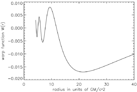
Figure 2: Warp function $W(r)$ for $a=0.5$. The sound speed is $0.01c$ and $W(r_{\mathrm{in}})=W_{0}=0.003$.

3.1.2 Coupling mechanism

The non-linearities in the basic equations (1) and (2) provide couplings between the different linear modes of the system. We are interested in those couplings that lead to amplification of the trapped modes. The basic idea of the excitation mechanism in warped discs (Kato, 2004) is that the warp interacts with a wave in the disc (the trapped r mode) giving rise to an intermediate mode. This intermediate mode can then couple with the warp to feed back on the original oscillations (see Fig. 3), resulting in growth of the latter.

For the r mode to be excited, it needs to gain energy in this coupling. Since the warp has null frequency, its energy is essentially zero and so the energy exchanges only happen between the r and the intermediate modes and the disc. It is widely agreed, and certainly true in the short-wavelength limit, although a general proof is lacking, that a mode that propagates inside its corotation radius has negative energy, i.e., the total energy of the disc is reduced in the presence of the wave, which is possible because the disc is rotating. On the other hand an axisymmetric wave, such as the r mode, or one that propagates outside its corotation radius, has positive energy. Suppose that, through coupling with the warp, the r mode generates an intermediate wave that propagates inside its corotation radius and therefore has negative energy. In the process of generating this wave, the r mode gains energy and is amplified. For sustained growth of the r mode, the intermediate wave must be damped so that its negative energy is continually replenished by the r mode. (The damping process itself draws positive energy from the rotation of the disc.) Therefore a dissipation term should be included in the equations for the intermediate mode. We choose to damp this wave locally at a rate $\beta\Omega$, where $\beta$ is a dimensionless parameter. The origin of this term is not discussed here but if we interpret it as some type of viscous dissipation or friction in the disc we expect the intermediate mode, which propagates in a larger region in the disc, to be more affected by it than the r mode, as the latter is trapped in a small region, and has a simpler radial structure. Also, the intermediate mode approaches its corotation radius (or the marginally stable orbit), where it is expected to be absorbed, and this effect is implicitly included in the intermediate mode equations when the friction term is included. Therefore, we neglect the dissipation term in the equations for the r mode. The growth rate that we obtain for the trapped mode should be compared with estimates of its damping rate due to turbulent viscosity.

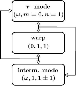
Figure 3: Diagram representing the interactions involved in the coupling mechanism involving a warped disc

.

For the coupling to occur the waves need to propagate in the same region in the disc and the parameters $\omega$ and $m$ for the 3 modes need to follow some basic coupling rules,

$$\omega_{\textrm{R}}\pm\omega_{\textrm{W}}=\omega_{\textrm{I}},\quad m_{\textrm{R}}\pm m_{\textrm{W}}=m_{\textrm{I}},$$ (28)

where the subscripts R, W and I refer to r mode, warp and intermediate mode quantities, respectively. These rules follow from the quadratic nature of the non-linearitites in the basic equations (1) and (2). Also, we can get information about the vertical mode number $n_{\textrm{I}}$ of the intermediate mode by remembering that the vertical dependence is given by Hermite polynomials. The warp quantities are proportional to $z$ and the simplest possible r mode has one node in the vertical direction, therefore its quantities are proportional to $\textrm{He}_{1}\sim z$. When the warp and this r mode interact, the coupling terms will be proportional to $z^{2}/H^{2}=(z^{2}/H^{2}-1)+1\sim\textrm{He}_{2}+\textrm{He}_{0}$, i.e., they give rise to two intermediate modes, one with 2 nodes in the vertical direction, $n_{\textrm{I}}=2$, and a 2D mode with $n_{\textrm{I}}=0$. We consider both possibilities. Note that the frequency of these intermediate waves is that of the r mode, and they are present because they are forced through the couplings. They could not exist as free waves satisfying the boundary conditions at this frequency.

According to rules (28), if $\omega_{\textrm{R}}=\omega$, then $\omega_{\textrm{I}}=\omega$. For the azimuthal mode numbers, we have $m_{\textrm{I}}=m_{\textrm{R}}\pm 1$. By analysing the propagation regions for these modes, and considering $\omega\approx\textrm{max}(\kappa+m\Omega)$, it is possible to conclude that the $n=0$ mode with $m_{\textrm{I}}=m_{\textrm{R}}-1$ and frequency $\omega$ does not have any Lindblad resonance, i.e., the point where the wave should be excited, in the disc. On the other hand, the mode with $m_{\textrm{R}}+1$ and frequency $\omega$ has an inner Lindblad resonance close to the region of propagation of the r mode. For these reasons, we choose the azimuthal mode number of the intermediate mode to be $m_{\textrm{R}}+1=1$, if the r mode is axisymmetric. This mode propagates inside its corotation resonance, while the r mode has positive energy. The presence of an inner Lindblad resonance means both that the intermediate mode attains a larger amplitude than it would in the case of nonresonant forcing, and that the flow of energy is such as to amplify the r mode.

If the vertical mode number of the intermediate mode is chosen to be 2 instead of 0, the r mode with $(\omega,m,n)=(\omega,0,1)$ interacts with a $(\omega,1,2)$ intermediate mode. The former propagates where $\omega^{2}<\kappa^{2}$, while the latter propagates where $(\omega-\Omega)^{2}<\kappa^{2}$, where $\omega$ is slightly less than $\max{(\kappa)}$. The propagation regions overlap close to the maximum of the epicyclic frequency since $\Omega\approx 2\kappa$ in this region.

The interaction of the r mode with the $n=2$ intermediate mode in a warped disc must be treated carefully because in this case the intermediate mode propagates between its Lindblad resonances and is absorbed at the corotation resonance. This is a radius in the disc where the potential $U(r)=-k^{2}$ tends to infinity and is therefore difficult to treat numerically because the wavelength tends to zero. One way of solving this problem is by including a relatively strong dissipation term in the equations for the intermediate mode. In this way the wave excited at the inner Lindblad resonance is damped before reaching corotation. This also works for the energy exchanges between the modes and the disc, since the $n=2$ mode has negative energy in the region where it is damped.

3.1.3 Results

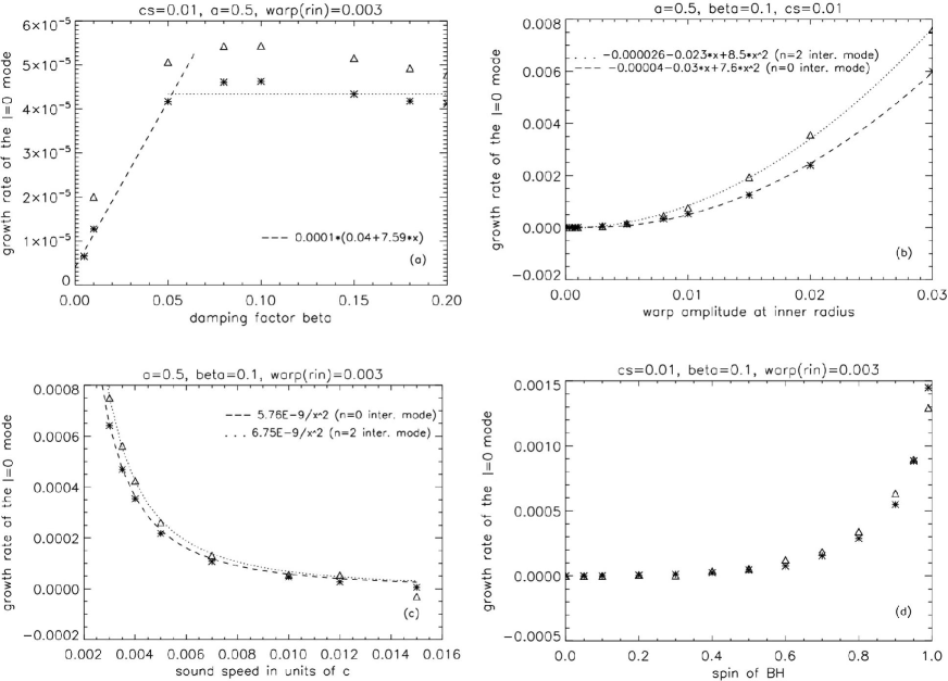
Figure 4: Variation of the growth rate of the simplest trapped r mode, $(l,m,n)=(0,0,1)$, with (a) dissipation factor $\beta$, (b) warp amplitude, $W$, at inner boundary, (c) sound speed in the disc, and (d) spin of the black hole. The triangles show the results for the interaction with the $n=2$ mode, while the stars are due to the interaction with the $n=0$ mode. For the former, the variation of the growth rate with the dissipation factor is not shown for small values of $\beta$ because of the influence of the corotation resonance in that case.

To find the r mode growth rate resulting from these interaction we solve the systems of coupled equations (60)–(66) and (67)–(74) (see Appendix A) for the interactions of the r mode with the $n=0$ and $n=2$ intermediate mode respectively. By considering the warp to have a fixed amplitude and neglecting the feedback of the r mode and intermediate modes on the warp, we still obtain a linear system of equations, although now the r mode and intermediate modes are coupled through the warp. We treat the $n=0$ and $n=2$ intermediate modes separately, although in practice both coupling mechanisms act simultaneously and the net growth rate is the sum of the rates due to the individual mechanisms.

We solve these systems numerically, using the Chebyshev method described in Section 2. For the r mode the same boundary conditions as before are used. Similar conditions are applied to the intermediate modes, i.e., $u_{\textrm{I}r}=0$ at $r_{\mathrm{in}}$ and $\textrm{d}u_{\textrm{I}r}/\textrm{d}r=\textrm{i}k_{\textrm{I}}u_{\textrm{I}r}$ at $r_{\mathrm{out}}$, where $k_{\textrm{I}}$ is given by the dispersion relation (14) at $r_{\mathrm{out}}$ for $m=1$ and $n=0$ or $n=2$, depending on the intermediate mode we are considering. As for the r mode, we choose the sign of $k_{\textrm{I}}$ so that the outgoing or exponentially decaying wave at $r_{\mathrm{out}}$ is chosen. The choice of the inner boundary condition for the radial component of the velocity of the $n=2$ mode is justified by the fact that this mode is exponentially decaying there. This choice is harder to justify for the $n=0$ mode since it is oscillatory at $r_{\mathrm{in}}$. This means that if $u_{\textrm{I}r}=0$ there then the wave is reflected at the inner boundary. Since the conditions at the marginally stable orbit are not clear, we cannot be sure of the physical validity of this condition; we choose it because of its simplicity. Rigorously we would need more boundary conditions to solve this problem, since more than 4 derivatives appear in each system. However, since the coupling terms are expected to be small, $u_{\textrm{R}\phi}$ is roughly proportional to $u_{\textrm{R}r}$ (and similarly for other quantities), thus the boundary conditions imposed for the latter will be indirectly imposed to the former.

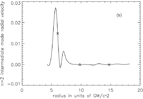
Figure 5: Variation of the real part of the radial component of the (a) $m=1$, $n=0$, and (b) $m=1$, $n=2$ intermediate mode velocity with radius for $c_{\mathrm{s}}/c=0.01$, $a=0.5$, $W(r_{\mathrm{in}})=0.003$, and $\beta=0.1$. The triangle indicates the radius of the corotation resonance, and the crosses the Lindblad resonances.

The aim is to find the frequencies $\omega$ for which the solutions corresponding to the r mode are trapped, i.e., for which $u_{\textrm{R}r}$ resembles the parabolic cylinder functions as in Fig. 1 (a), which is expected if the coupling terms are small when compared to the other terms in the equations. The imaginary part of $\omega$ then gives the growth rate (or damping rate, if it’s negative) of the trapped r mode. In Fig. 5 we show the $n=0$ and $n=2$ intermediate modes involved in the coupling process, when the dissipation is strong. It should be noted that when the dissipation is weak, the $n=2$ intermediate mode develops a very short wavelength as it approaches the corotation resonance. If $\beta$ is too small, the length-scale on which this wave dissipates is not resolved by our numerical method. The variation of the growth rate with several parameters is shown in Fig. 4. These results are discussed in Section 4.

3.2 Eccentric discs

Another possible mechanism for the excitation of trapped waves is their interaction with an eccentric disc (Kato, 2007). Interacting binary stars with mass ratio $q\la 0.3$ are believed to have eccentric accretion discs. This phenomenon is well documented in the case of cataclysmic variable stars, where superhumps are observed during the superoutbursts of the SU UMa class of dwarf novae (Patterson et al., 2005) and in other systems of low mass ratio. In these systems, a resonant interaction of the orbiting gas with the tidal potential of the companion star allows a growth of eccentricity (Whitehurst, 1988; Lubow, 1991a, b). Superhumps are also observed in an increasing number of low-mass X-ray binaries, and systems exhibiting black-hole HFQPOs are likely to have mass ratios $q\la 0.3$ and therefore to have eccentric discs during at least some phases of their outbursts.

Recently, Kato (2007) argued that one-armed global oscillations, symmetric with respect to the $z=0$ plane, can excite trapped oscillations. His conclusions are based on analytical, Lagrangian calculations and are too crude to allow for more than simple estimates for the growth rates. In this section we describe an excitation mechanism similar to the one reported previously, but where an $(m=1,n=0)$ eccentric mode has the role that previously belonged to the $(m=1,n=1)$ warp wave. Using the same numerical method as before, we calculate the trapped r mode growth rates.

3.2.1 Variation of eccentricity with radius

As before, consider the set of equations (10)–(13). A global eccentric mode corresponds to a zero-frequency wave with $m=1$ and $n=0$. (If the global eccentric mode precesses freely, the frequency is not exactly zero but is completely negligible compared to the characteristic frequencies in the inner part of the disc.) In this case, equations (10)–(13) are, after the usual separation of variables, reduced to

$$\textrm{i}\Omega u_{\textrm{E}r}-2\Omega u_{\textrm{E}\phi}=-\frac{\textrm{d}h_{\textrm{E}}}{\textrm{d}r},$$ (29)

$$\textrm{i}\Omega u_{\textrm{E}\phi}+\frac{\kappa^{2}}{2\Omega}=-\textrm{i}\frac{h_{\textrm{E}}}{r},$$ (30)

$$\textrm{i}\Omega u_{\textrm{E}z}=0,$$ (31)

$$\textrm{i}\Omega h_{\textrm{E}}=-c_{\mathrm{s}}^{2}\left[\frac{1}{r}\frac{\textrm{d}}{\textrm{d}r}(ru_{\textrm{E}r})+\textrm{i}\frac{u_{\textrm{E}\phi}}{r}\right],$$ (32)

where the subscript E refers to eccentric mode quantities. This system admits a solution of the form

$$u_{\textrm{E}r}=\textrm{i}E\Omega r,$$ (33)

$$u_{\textrm{E}\phi}=\frac{c_{\mathrm{s}}^{2}r^{2}\Omega}{\Omega^{2}r^{2}-c_{\mathrm{s}}^{2}}\frac{\textrm{d}E}{\textrm{d}r}-\frac{\kappa^{2}}{2}rE,$$ (34)

$$u_{\textrm{E}z}=0,$$ (35)

$$h_{\textrm{E}}=-\frac{c_{\mathrm{s}}^{2}r^{2}\Omega}{\Omega^{2}r^{2}-c_{\mathrm{s}}^{2}}\frac{\textrm{d}E}{\textrm{d}r},$$ (36)

where $E(r)$ is the eccentricity of the disc at radius $r$, and satisfies

$$(\kappa^{2}-\Omega^{2})E=\frac{1}{r^{3}}\frac{\textrm{d}}{\textrm{d}r}\left(\frac{r^{5}c_{\mathrm{s}}^{2}\Omega^{2}}{\Omega^{2}r^{2}-c_{\mathrm{s}}^{2}}\frac{\textrm{d}E}{\textrm{d}r}\right).$$ (37)

Again, this equation is closely related, but not identical, to equation (21) of Goodchild & Ogilvie (2006), which was derived from an analysis of global eccentricity in a two-dimensional disc. Radially propagating solutions are obtained because $\kappa^{2}<\Omega^{2}$ in a relativistic disc. As for the warp tilt $W(r)$, we solve this equation numerically, using a 4th order Runge–Kutta method with boundary conditions $E(r_{\mathrm{in}})=E_{0}$, and $\textrm{d}E/\textrm{d}r(r_{\mathrm{in}})=0$, where $E_{0}$ is an arbitrary value for the eccentricity at the inner boundary, i.e., at the marginally stable orbit. A typical solution for $E(r)$ is shown in Fig. 6. The eccentricity has an oscillatory behaviour, with the wavelength decreasing with radius, consistent with the local dispersion relation. Again, we defer to a second paper a more realistic treatment of the propagation of the eccentricity into the inner part of the disc.

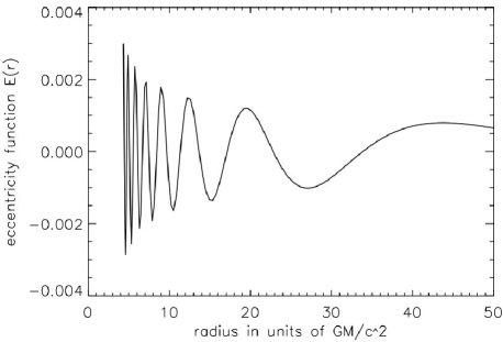
Figure 6: Eccentricity function $E(r)$ for $a=0.5$. The sound speed is $0.01c$ and $E(r_{\mathrm{in}})=E_{0}=0.003$.

3.2.2 Coupling mechanism

The excitation mechanism is similar to the one discussed in the previous section: a global deformation mode, which is now the eccentricity mode, characterized by $(\omega,m,n)=(0,1,0)$, interacts with a trapped r mode $(\omega,0,1)$ giving rise to an intermediate mode. The latter then couples with the global mode to feedback on to the trapped r mode.

Coupling rules require the intermediate mode to have the same frequency as the trapped wave and, as before, we have $m_{\textrm{I}}=1$, in the case where the trapped r mode is axisymmetric. As for the vertical dependence, since the eccentric mode has $n=0$, the intermediate mode can only have the same vertical mode number as the trapped mode, i.e., $n_{\textrm{I}}=1$. The propagation region for this mode is the same as for the $(\omega,1,2)$ intermediate mode, present in the interaction of the r mode with the warp. As in that case, a relatively large damping term must be included in the equations for the intermediate mode so that it dissipates on a resolved scale before reaching the corotation resonance. In this case the energy exchanges are similar to the ones discussed for the interaction in a warped disc.

To find the growth rates that result from this interaction, we solve equations (75)–(82), using the same numerical method and boundary conditions as before.

The variation of the growth rate with the inner eccentricity, sound speed, spin of black hole and dissipation factor is shown in Fig. 7. The values of the growth rate achieved in the interaction of the trapped wave with the eccentric mode are, in general, similar to the values obtained in the interaction with the warp, if the inner inclination and eccentricity are similar.

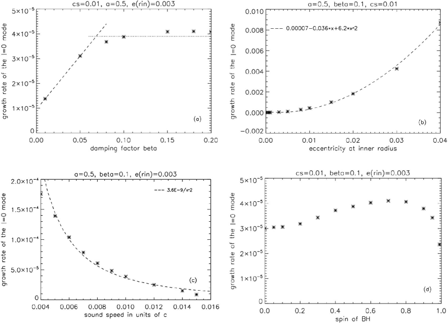
Figure 7: Variation of the growth rate of the simplest trapped r mode, $(l,m,n)=(0,0,1)$, with (a) dissipation factor $\beta$, (b) eccentricity amplitude, $E$, at inner boundary, (c) sound speed of the disc, and (d) spin of the black hole.

4 Discussion

In this section we discuss the results shown in Figs 4 and 7, where the dependence of the $l=0$ r mode growth rate with several parameters is represented.

4.1 Growth rates in warped discs

In the variation of the growth rate with the dissipation factor, two regimes can be considered: weak dissipation ($\beta\lesssim 0.05$), where the variation is approximately linear, and strong dissipation ($\beta\gtrsim 0.05$), where the growth rate remains approximately constant when $\beta$ varies (Fig. 4 (a)). In the former case, the $n=0$ intermediate mode is launched at its inner Lindblad resonance and propagates, being slightly attentuated, until it reaches the inner boundary where it is reflected. Owing to the attenuation, the reflected wave amplitude is smaller than the incident one, and therefore the intermediate mode does not cancel itself, leaving a small amount of energy available for the r mode to be excited. In the strong dissipation regime, the $n=0$ mode is dissipated before reaching the marginally stable orbit. In this case, all the energy carried by this wave becomes available to excite the trapped mode. As for the $n=2$ intermediate mode, in the strong dissipation regime, the wave is completely dissipated before reaching the corotation resonance. Physically we would expect no dissipation term to be necessary in this case. An arbitrarily small amount of dissipation should lead in principle to the complete absorption of the wave at the corotation resonance. However, this cannot be verified numerically because of the difficulty in resolving the wavelength of the intermediate mode as the singularity at the corotation resonance is approached.

For small warp amplitudes, i.e., before the coupling terms start affecting the structure of the eigenfunctions, the growth rate grows with the square of the warp amplitude at the inner boundary (Fig. 4 (b)). This is expected since the coupling mechanism relies on the ‘use’ of the warp twice: first on the interaction with the r mode to give rise to the intermediate modes, and then again on the interaction with the latter to feed back on the former (Fig. 3).

The excitation mechanism discussed here is similar to the well known parametric instability, in the case where one of the modes is strongly damped. The parametric instability is a type of resonant coupling between three modes satisfying $\omega_{\textrm{p}}\approx\omega_{\textrm{d}1}+\omega_{\textrm{d}2}$, where the subscripts p and d refer to parent and daughter modes, respectively. The parametric instability results in the transfer of energy from the former to the latter, when the daughter modes have small amplitude. The equations describing the evolution of the mode amplitudes read (Wu & Goldreich, 2001, adapted from),

$$\frac{\textrm{d}A_{\textrm{p}}}{\textrm{d}t}=+\gamma_{\textrm{p}}A_{\textrm{p}}-\textrm{i}\omega_{\textrm{p}}A_{\textrm{p}}+\textrm{i}\omega_{\textrm{p}}\sigma A_{\textrm{d}1}A_{\textrm{d}2},$$ (38)

$$\frac{\textrm{d}A_{\textrm{d}1}}{\textrm{d}t}=-\gamma_{\textrm{d}1}A_{\textrm{d}1}-\textrm{i}\omega_{\textrm{d}1}A_{\textrm{d}1}+\textrm{i}\omega_{\textrm{d}1}\sigma A_{\textrm{p}}A^{*}_{\textrm{d}2},$$ (39)

$$\frac{\textrm{d}A_{\textrm{d}2}}{\textrm{d}t}=-\gamma_{\textrm{d}2}A_{\textrm{d}2}-\textrm{i}\omega_{\textrm{d}2}A_{\textrm{d}2}+\textrm{i}\omega_{\textrm{d}2}\sigma A^{*}_{\textrm{d}1}A_{\textrm{p}},$$ (40)

where $\gamma_{j}>0$ is the linear amplitude growth/damping rate of mode $j$ and $\sigma$ is the non-linear coupling constant. Let us consider a simplified case where the amplitude of the parent mode is approximately constant in time (because the daughter modes are of small amplitude), and $\omega_{\textrm{d}1}=-\omega_{\textrm{d}2}=\omega$, $\gamma_{\textrm{p}}=\gamma_{\textrm{d}1}=0$ and $\gamma_{\textrm{d}2}=\gamma$. In this case, the parent mode can be compared to the warp while the daughter modes 1 and 2 can be compared with the r and intermediate modes, respectively. Assuming $A_{\textrm{d}1}\propto\exp{(st)}$, the growth rate is

$$\textrm{Re}(s)=-\frac{\gamma}{2}+\left(\frac{\gamma^{2}}{4}+|A_{\textrm{p}}|^{2}\sigma^{2}\omega^{2}\right)^{1/2}.$$ (41)

If $\gamma\ll|A_{\mathrm{p}}|\sigma\omega$, $\textrm{Re}(s)\approx|A_{\textrm{p}}|\sigma\omega-\frac{\gamma}{2}$, i.e., the growth rate is linearly related to the amplitude of the parent mode. On the other hand, if $\gamma\gg|A_{\mathrm{p}}|\sigma\omega$, $\textrm{Re}(s)\approx|A_{\mathrm{p}}|^{2}\sigma^{2}\omega^{2}/\gamma$, i.e., the growth rate is proportional to the square of the amplitude of the parent mode. The latter case is the one similar to the excitation mechanism we are discussing here. It should be noted that this parametric instability analysis gives a dependence of the growth rate in $\gamma$ which is not in agreement with the numerical results (considering $\gamma$ to be equivalent to $\beta$), because the dependence of the spatial structure of the intermediate mode on the dissipation is not considered in this simplistic analysis. Also, the parametric instability analysis suggests that the daughter modes gain energy from the parent mode, which is not what happens in the coupling mechanism we are considering, since here the differential rotation of the disc, and not the warp, is the ultimate source of energy for the r mode. Although the parametric instability analysis gives a dependence of the growth rate on the disturbance amplitude in agreement with our numerical results, it is simplistic and does not consider all the details of the coupling mechanism. A parallel between the parametric instability and our excitation mechanism is therefore not straightforward.

In the strong dissipation regime, the intermediate mode dissipates completely, and does not influence the variation of the r mode growth rate with both the sound speed of the disc and the spin of the black hole. In this regime, the growth rate decreases with increasing $c_{\mathrm{s}}$, as expected. The hotter the disc is, the wider the modes get, which means that if the sound speed is high, the modes are not as well trapped. More importantly, the shape of the warp changes when the sound speed changes since its wavelength ($\lambda_{\textrm{W}}$) is proportional to $c_{\textrm{s}}$. The interaction relies on the use of the warp twice, therefore we can argue that the growth rate is proportional to $|dW/dr|^{2}$ (since $W$ represents the inclination and $dW/dr$ the actual warp). Since $|dW/dr|^{2}\propto W_{0}^{2}/\lambda_{\textrm{W}}^{2}\propto W_{0}^{2}/c_{\textrm{s}}^{2}$, i.e., for fixed sound speed the growth rate is proportional to the square of the inner warp amplitude (Fig. 4 (b)) and for fixed $W_{0}$, the growth rate varies with $1/c_{\textrm{s}}^{2}$ (Fig. 4 (c)). The small changes to the $1/c_{\mathrm{s}}^{2}$ law are justified by the fact that, for large sound speed, the decay rate due to the ‘leakage’ at $r_{\textrm{out}}$ is considerable.

As for the variation of the growth rate with the spin of the black hole, an important conclusion is that, in fact, as argued in the beginning of this section, there is no mode excitation if the black hole is non-rotating. This was not evident in Kato’s simple estimates for the growth rates. The fact that the growth rate increases with $a$ is also expected, not only because the waves are better confined for larger values of $a$, but mainly because the average warp amplitude in the trapped region is larger, for larger $a$. Also, the wavelength of the warp decreases as $a$ increases, because the Lense–Thirring frequency ($\Omega_{\textrm{LT}}=\Omega-\Omega_{z}\approx 2a/r^{3}$) increases. Therefore, for the same inner $W$, a larger $dW/dr$ is achieved. In light of these very preliminary results, we could argue that HFQPOs would preferentially be detected in black hole candidates with large spin, if the interaction of the trapped r mode with a warped disc is the mechanism responsible for the excitation of the former.

4.2 Growth rates in eccentric discs

For the interaction between the r and intermediate modes in an eccentric disc, the variation of the growth rate with the dissipation factor is similar to the same variation for the interaction in a warped disc (Figs 7 (a) and 4 (a)). Also, the change of the growth rate with the inner eccentricity (Fig. 7 (b)) is very similar to the variation of the growth rate with the warp tilt at the inner radius, i.e., there is a square dependence on the eccentricity amplitude at $r_{\mathrm{in}}$. This is expected as the eccentric mode plays, in the wave interaction described in this section, the role of the warp in the interactions described previously. Similarly, the variation with the sound speed (Fig. 7 (c)) is also the expected one.

The main difference between the interaction with the warp and the interaction with the eccentric mode is in the variation of the growth rate with the spin of the black hole (Fig. 7 (d)). The warp, being a $n=1$ mode, has a variation with radius that strongly depends on the Lense-Thirring precession frequency, and therefore, that strongly depends on $a$. On the other hand, the variation of the eccentricity amplitude with radius, given by equation (37), is less dependent on the spin of the black hole. Therefore, the variation of $a$ only causes variations of a factor of, at maximum, $2$ in the growth rate obtained for the interaction within the eccentric disc. A very important difference is the fact that, in this interaction, a reasonable growth rate can be obtained in the case where $a=0$. Therefore, in slowly rotating black holes, HFQPOs might be detected if the disc is eccentric, and if this excitation mechanism is responsible for the increase in the amplitude of oscillations.

5 Conclusions

In this paper we have described an excitation mechanism for trapped inertial modes, based on a non-linear coupling mechanism between these waves and global deformations (warping or eccentricity) in accretion discs. We have seen that the interaction of a trapped r mode with an intermediate mode and a deformation in the disc results in growth of the trapped mode, if there is some process capable of making the intermediate mode dissipate in the disc. Dissipation is required so that this mode can remove rotational kinetic energy from the disc, which becomes available for the r mode to grow. Depending on the values of the sound speed, spin of the black hole and amplitude of the deformation at the inner radius, reasonable growth rates can be obtained for a warp or eccentricity of modest amplitude. In a warped disc, where the growth rate varies significantly with the spin of the compact object, growth rates as large as $\omega/10$, where $\omega$ is the oscillation frequency, can be obtained. If $a=0$, no oscillations are excited in these discs. However, it may still possible to excite trapped modes in discs around non-rotating black holes if they are eccentric.

The coupling process described here works as an excitation mechanism for trapped inertial waves, under a wide range of conditions, provided global deformations reach the inner disc region with non-negligible amplitude. The propagation of global modes, in a more realistic disc model, is the subject of a forthcoming paper (Ferreira & Ogilvie, 2008).

In this paper we considered the excitation of trapped waves due to a non-linear coupling mechanism with global deformations, in a simple disc model. While this effect is responsible for the growth of these modes, it has to compete with others that contribute to the damping of these waves. For example, since the conditions at the marginally stable orbit are unknown, it is possible for a ‘leakage’ of the trapped mode (similar to the one considered in the potential barrier analogy) through $r_{\textrm{ms}}$ to exist. This effect is to be considered in the future. Also, and more importantly, viscous dissipation in the disc can cause damping of these modes. A simple estimate gives a damping rate of $\alpha\Omega$. For small enough values of $\alpha$ and large enough warp or eccentricity, net growth can occur.

Another point to be discussed is the applicability of our results to observed discs. We consider a very simple, isothermal disc model and wave perturbations for which $\gamma=1$. In a more realistic disc, the vertical structure of the waves is changed while they propagate radially. The wave energy concentrates either near the surface of the disc (Lubow & Ogilvie, 1998) or towards the disc mid-plane (Korycansky & Pringle, 1995), which could potentially hinder the propagation of intermediate modes away from the Lindblad resonance where they are excited. However, the process of ‘wave channelling’ mentioned by Lubow & Ogilvie (1998) is only relevant at a distance from the resonance of $\sim r_{\textrm{L}}/m$ ($r_{\textrm{L}}$ being the radius of the Lindblad resonance), where the radial wavelength becomes comparable to the semithickness of the disc. Since the intermediate modes have $m=1$, this effect is not important in the region where wave coupling occurs. The same is expected for cases in which the energy concentrates towards the disc mid-plane. The global deformation modes do not undergo significant wave channelling because their wavelengths are always long compared to $H$. Therefore, we believe that our results, obtained in a simple disc model, are still qualitatively valid in more realistic discs.

Appendix A Non-linear coupling equations

A.1 Wave coupling in a warped disc

The following system of equations (cf. equations (1)–(2)) describes the propagation of the r mode and $n=0$ intermediate mode, coupled by the warp, and needs to be solved for the growth rate to be determined:

$$\left(\frac{\partial}{\partial t}+\Omega\frac{\partial}{\partial\phi}\right)u^{\prime}_{\textrm{R}r}-2\Omega u^{\prime}_{\textrm{R}\phi}=-\frac{\partial h^{\prime}_{\textrm{R}}}{\partial r}+f_{\textrm{R}r},$$ (42)

$$\left(\frac{\partial}{\partial t}+\Omega\frac{\partial}{\partial\phi}\right)u^{\prime}_{\textrm{R}\phi}+\frac{\kappa^{2}}{2\Omega}u^{\prime}_{\textrm{R}r}=-\frac{1}{r}\frac{\partial h^{\prime}_{\textrm{R}}}{\partial\phi}+f_{\textrm{R}\phi},$$ (43)

$$\left(\frac{\partial}{\partial t}+\Omega\frac{\partial}{\partial\phi}\right)u^{\prime}_{\textrm{R}z}=-\frac{\partial h^{\prime}_{\textrm{R}}}{\partial z}+f_{\textrm{R}z},$$ (44)

$$\left(\frac{\partial}{\partial t}+\Omega\frac{\partial}{\partial\phi}\right)h^{\prime}_{\textrm{R}}-\Omega_{z}^{2}zu^{\prime}_{\textrm{R}z}=-c_{\mathrm{s}}^{2}\left[\frac{1}{r}\frac{\partial(ru^{\prime}_{\textrm{R}r})}{\partial r}+\frac{1}{r}\frac{\partial u^{\prime}_{\textrm{R}\phi}}{\partial\phi}+\frac{\partial u^{\prime}_{\textrm{R}z}}{\partial z}\right]+f_{\textrm{R}h},$$ (45)

$$\left(\frac{\partial}{\partial t}+\Omega\frac{\partial}{\partial\phi}\right)u^{\prime}_{\textrm{I}r}-2\Omega u^{\prime}_{\textrm{I}\phi}=-\frac{\partial h^{\prime}_{\textrm{I}}}{\partial r}-\beta\Omega u^{\prime}_{\textrm{I}r}+f_{\textrm{I}r},$$ (46)

$$\left(\frac{\partial}{\partial t}+\Omega\frac{\partial}{\partial\phi}\right)u^{\prime}_{\textrm{I}\phi}+\frac{\kappa^{2}}{2\Omega}u^{\prime}_{\textrm{I}r}=-\frac{1}{r}\frac{\partial h^{\prime}_{\textrm{I}}}{\partial\phi}-\beta\Omega u^{\prime}_{\textrm{I}\phi}+f_{\textrm{I}\phi},$$ (47)

$$\left(\frac{\partial}{\partial t}+\Omega\frac{\partial}{\partial\phi}\right)h^{\prime}_{\textrm{I}}=-c_{\mathrm{s}}^{2}\left[\frac{1}{r}\frac{\partial(ru^{\prime}_{\textrm{R}r})}{\partial r}+\frac{1}{r}\frac{\partial u^{\prime}_{\textrm{I}\phi}}{\partial\phi}\right]-\beta\Omega h^{\prime}_{\textrm{I}}+f_{\textrm{I}h},$$ (48)

where

$$\mn@boldsymbol{f}_{\textrm{R}}=\left(f_{\textrm{R}r},f_{\textrm{R}\phi},f_{\textrm{R}z}\right)=-\mn@boldsymbol{u}^{\prime}_{\textrm{I}}\cdot\nabla\mn@boldsymbol{u}^{\prime}_{\textrm{W}}-\mn@boldsymbol{u}^{\prime}_{\textrm{W}}\cdot\nabla\mn@boldsymbol{u}^{\prime}_{\textrm{I}},$$ (49)

$$f_{\textrm{R}h}=-\mn@boldsymbol{u}^{\prime}_{\textrm{I}}\cdot\nabla h^{\prime}_{\textrm{W}}-\mn@boldsymbol{u}^{\prime}_{\textrm{W}}\cdot\nabla h^{\prime}_{\textrm{I}},$$ (50)

$$\mn@boldsymbol{f}_{\textrm{I}}=\left(f_{\textrm{I}r},f_{\textrm{I}\phi},f_{\textrm{I}z}\right)=-\mn@boldsymbol{u}^{\prime}_{\textrm{R}}\cdot\nabla\mn@boldsymbol{u}^{\prime}_{\textrm{W}}-\mn@boldsymbol{u}^{\prime}_{\textrm{W}}\cdot\nabla\mn@boldsymbol{u}^{\prime}_{\textrm{R}},$$ (51)

$$f_{\textrm{I}h}=-\mn@boldsymbol{u}^{\prime}_{\textrm{R}}\cdot\nabla h^{\prime}_{\textrm{W}}-\mn@boldsymbol{u}^{\prime}_{\textrm{W}}\cdot\nabla h^{\prime}_{\textrm{R}}$$ (52)

are the coupling terms, arising from non-linearities in the basic equations.

Since we are interested in studying the axisymmetric r mode, the azimuthal mode number for the intermediate mode is $1$. Also, since the simplest possible r mode has one node in the vertical direction and the intermediate mode has $n=0$, we use the following separation of variables:

$$(u^{\prime}_{\textrm{R}r},u^{\prime}_{\textrm{R}\phi},h^{\prime}_{\textrm{R}})=\textrm{Re}\left[\left(u_{\textrm{R}r}(r),u_{\textrm{R}\phi}(r),h_{\textrm{R}}(r)\right)\textrm{He}_{1}\left(\frac{z}{H}\right)\textrm{e}^{-\textrm{i}\omega t}\right],$$ (53)

$$u^{\prime}_{\textrm{R}z}=\textrm{Re}\left[u_{\textrm{R}z}(r)\textrm{He}_{0}\left(\frac{z}{H}\right)\textrm{e}^{-\textrm{i}\omega t}\right],$$ (54)

$$(u^{\prime}_{\textrm{I}r},u^{\prime}_{\textrm{I}\phi},h^{\prime}_{\textrm{I}})=\textrm{Re}\left[\left(u_{\textrm{I}r}(r),u_{\textrm{I}\phi}(r),h_{\textrm{I}}(r)\right)\textrm{He}_{0}\left(\frac{z}{H}\right)\textrm{e}^{\textrm{i}\phi-\textrm{i}\omega t}\right],$$ (55)

$$u^{\prime}_{\textrm{I}z}=0\quad\textrm{(2D mode)},$$ (56)

$$(u^{\prime}_{\textrm{W}r},u^{\prime}_{\textrm{W}\phi},h^{\prime}_{\textrm{W}})=\textrm{Re}\left[\left(u_{\textrm{W}r}(r),u_{\textrm{W}\phi}(r),h_{\textrm{W}}(r)\right)z\,\textrm{e}^{\textrm{i}\phi}\right],$$ (57)

$$u^{\prime}_{\textrm{W}z}=\textrm{Re}\left[u_{\textrm{W}z}(r)\,\textrm{e}^{\textrm{i}\phi}\right].$$ (58)

This separation of variables results in having the coupling terms (49) and (50) proportional to $\textrm{He}_{1}$ only, while the coupling terms (51)–(52) give rise to terms proportional to both $\textrm{He}_{0}=1$ and $\textrm{He}_{2}=z^{2}/H^{2}-1$. Since we are interested in the terms that influence the mode with $n=0$, we need to project these forcing terms on to $\textrm{He}_{0}$. Also, the separation of variables results in coupling terms of the form

$$\textrm{Re}(A)\textrm{Re}(B)=\frac{1}{2}\textrm{Re}(AB+AB^{*}),$$ (59)

which means that the interaction of the $m=0$ r mode with the $m=1$ warp results in two new modes, one with $m=1$ and one with $m=-1$:

$$r\textrm{-mode }(A)\propto\textrm{e}^{-\textrm{i}\omega t}\quad\textrm{and}\quad\textrm{warp }(B)\propto\textrm{e}^{\textrm{i}\phi}$$

$$\Rightarrow\quad r\textrm{-mode }\times\textrm{ warp}\propto AB+AB^{*}\propto\textrm{e}^{\textrm{i}\phi-\textrm{i}\omega t}+\textrm{e}^{-\textrm{i}\phi-\textrm{i}\omega t}.$$

Since we are only interested in the action of this coupling on the intermediate mode with $m=1$, because the one with $m=-1$ does not have any Lindblad resonances (location where the wave should be excited) in the disc, these forcing terms are projected on to $\textrm{e}^{\textrm{i}\phi-\textrm{i}\omega t}$. Similarly, the interaction of the intermediate mode with the warp gives rise to a $m=2$ mode in addition to the axisymmetric r mode we are interested in:

$$\textrm{intermediate mode }(A)\propto\textrm{e}^{\textrm{i}\phi-\textrm{i}\omega t}\quad\textrm{and}\quad\textrm{warp }(B)\propto\textrm{e}^{\textrm{i}\phi}$$

$$\Rightarrow\quad\textrm{intermediate mode }\times\textrm{ warp}\propto AB+AB^{*}\propto\textrm{e}^{\textrm{i}2\phi-\textrm{i}\omega t}+\textrm{e}^{-\textrm{i}\omega t}.$$

Therefore, these forcing terms should be projected on to $\textrm{e}^{-\textrm{i}\omega t}$, which means that complex conjugates of warp quantities will appear in the equations.

After separating variables, and projecting the forcing terms appropriately, the equations to be solved can be written as

$$-\textrm{i}\omega u_{\textrm{R}r}=2\Omega u_{\textrm{R}\phi}-\frac{\textrm{d}h_{\textrm{R}}}{\textrm{d}r}-\frac{u_{\textrm{I}r}}{2}\frac{\textrm{d}u^{*}_{\textrm{W}r}}{\textrm{d}r}H+\textrm{i}u_{\textrm{I}\phi}\frac{u^{*}_{\textrm{W}r}}{2r}H+u_{\textrm{I}\phi}\frac{u^{*}_{\textrm{W}\phi}}{r}H-\frac{u^{*}_{\textrm{W}r}}{2}\frac{\textrm{d}u_{\textrm{I}r}}{\textrm{d}r}H-\textrm{i}u^{*}_{\textrm{W}\phi}\frac{u_{\textrm{I}r}}{2r}H$$ (60)

$$-\textrm{i}\omega u_{\textrm{R}\phi}=-\frac{\kappa^{2}}{2\Omega}u_{\textrm{R}r}-\frac{u_{\textrm{I}r}}{2}\frac{\textrm{d}u^{*}_{\textrm{W}\phi}}{\textrm{d}r}H-u_{\textrm{I}\phi}\frac{u^{*}_{\textrm{W}r}}{2r}H-\frac{u^{*}_{\textrm{W}r}}{2}\frac{\textrm{d}u_{\textrm{I}\phi}}{\textrm{d}r}H-u^{*}_{\textrm{W}\phi}\frac{u_{\textrm{I}r}}{2r}H$$ (61)

$$-\textrm{i}\omega u_{\textrm{R}z}=-\frac{h_{\textrm{R}}}{H}-\frac{u_{\textrm{I}r}}{2}\frac{\textrm{d}u^{*}_{\textrm{W}z}}{\textrm{d}r}+\textrm{i}u_{\textrm{I}\phi}\frac{u^{*}_{\textrm{W}z}}{2r}$$ (62)

$$-\textrm{i}\omega h_{\textrm{R}}=\Omega_{z}^{2}Hu_{\textrm{R}z}-\frac{c_{\mathrm{s}}^{2}}{r}\frac{\textrm{d}(ru_{\textrm{R}r})}{\textrm{d}r}-\frac{u_{\textrm{I}r}}{2}\frac{\textrm{d}h^{*}_{\textrm{W}}}{\textrm{d}r}H+\textrm{i}u_{\textrm{I}\phi}\frac{h^{*}_{\textrm{W}}}{2r}H-\frac{u^{*}_{\textrm{W}r}}{2}\frac{\textrm{d}h_{\textrm{I}}}{\textrm{d}r}H-\textrm{i}u^{*}_{\textrm{W}\phi}\frac{h_{\textrm{I}}}{2r}H$$ (63)

$$-\textrm{i}\omega u_{\textrm{I}r}=-(\textrm{i}+\beta)\Omega u_{\textrm{I}r}+2\Omega u_{\textrm{I}\phi}-\frac{\textrm{d}h_{\textrm{I}}}{\textrm{d}r}-\frac{u_{\textrm{R}r}}{2}\frac{\textrm{d}u_{\textrm{W}r}}{\textrm{d}r}H-\textrm{i}u_{\textrm{R}\phi}\frac{u_{\textrm{W}r}}{2r}H+u_{\textrm{R}\phi}\frac{u_{\textrm{W}\phi}}{r}H-u_{\textrm{R}r}\frac{u_{\textrm{W}z}}{2H}-\frac{u_{\textrm{W}r}}{2}\frac{\textrm{d}u_{\textrm{R}r}}{\textrm{d}r}H$$

$$-u_{\textrm{R}z}\frac{u_{\textrm{W}r}}{2}$$ (64)

$$-\textrm{i}\omega u_{\textrm{I}\phi}=-(\textrm{i}+\beta)\Omega u_{\textrm{I}\phi}-\frac{\kappa^{2}}{2\Omega}u_{\textrm{I}r}-\frac{\textrm{i}h_{\textrm{I}}}{r}-\frac{u_{\textrm{R}r}}{2}\frac{\textrm{d}u_{\textrm{W}\phi}}{\textrm{d}r}H-\textrm{i}u_{\textrm{R}\phi}\frac{u_{\textrm{W}\phi}}{2r}H-u_{\textrm{R}\phi}\frac{u_{\textrm{W}r}}{2r}H-\frac{u_{\textrm{W}r}}{2}\frac{\textrm{d}u_{\textrm{R}\phi}}{\textrm{d}r}H-u_{\textrm{W}\phi}\frac{u_{\textrm{R}r}}{2r}H$$

$$-u_{\textrm{R}z}\frac{u_{\textrm{W}\phi}}{2}-u_{\textrm{W}z}\frac{u_{\textrm{R}\phi}}{2H}$$ (65)

$$-\textrm{i}\omega h_{\textrm{I}}=-(\textrm{i}+\beta)\Omega h_{\textrm{I}}-\frac{c_{\mathrm{s}}^{2}}{r}\frac{\textrm{d}(ru_{\textrm{I}r})}{\textrm{d}r}-c_{\mathrm{s}}^{2}\frac{\textrm{i}u_{\textrm{I}\phi}}{r}-\frac{u_{\textrm{R}r}}{2}\frac{\textrm{d}h_{\textrm{W}}}{\textrm{d}r}H-\textrm{i}u_{\textrm{R}\phi}\frac{h_{\textrm{W}}}{2r}H-\frac{u_{\textrm{W}r}}{2}\frac{\textrm{d}h_{\textrm{R}}}{\textrm{d}r}H-u_{\textrm{W}z}\frac{h_{\textrm{R}}}{2H}-u_{\textrm{R}z}\frac{h_{\textrm{W}}}{2}.$$ (66)

This system is linear in the unknowns for the r and intermediate modes. The warp, which couples these modes together, is assumed to be known.

For the interaction with the $n=2$ intermediate mode, similar equations need to be solved. After separating variables and projecting forcing terms appropriately, the equations describing this interaction read

$$-\textrm{i}\omega u_{\textrm{R}r}=2\Omega u_{\textrm{R}\phi}-\frac{\textrm{d}h_{\textrm{R}}}{\textrm{d}r}-u_{\textrm{I}r}\frac{\textrm{d}u^{*}_{\textrm{W}r}}{\textrm{d}r}H+\textrm{i}u_{\textrm{I}\phi}\frac{u^{*}_{\textrm{W}r}}{r}H+2u_{\textrm{I}\phi}\frac{u^{*}_{\textrm{W}\phi}}{r}H-u^{*}_{\textrm{W}r}\frac{\textrm{d}u_{\textrm{I}r}}{\textrm{d}r}H-\textrm{i}u^{*}_{\textrm{W}\phi}\frac{u_{\textrm{I}r}}{r}H-\frac{u^{*}_{\textrm{W}z}}{H}u_{\textrm{I}r}+\frac{u^{*}_{\textrm{W}r}}{2}u_{\textrm{I}z}$$ (67)

$$-\textrm{i}\omega u_{\textrm{R}\phi}=-\frac{\kappa^{2}}{2\Omega}u_{\textrm{R}r}-u_{\textrm{I}r}\frac{\textrm{d}u^{*}_{\textrm{W}\phi}}{\textrm{d}r}H-u_{\textrm{I}\phi}\frac{u^{*}_{\textrm{W}r}}{r}H-u^{*}_{\textrm{W}r}\frac{\textrm{d}u_{\textrm{I}\phi}}{\textrm{d}r}H-u^{*}_{\textrm{W}\phi}\frac{u_{\textrm{I}r}}{r}H-\frac{u^{*}_{\textrm{W}z}}{H}u_{\textrm{I}\phi}+\frac{u^{*}_{\textrm{W}\phi}}{2}u_{\textrm{I}z}$$ (68)

$$-\textrm{i}\omega u_{\textrm{R}z}=-\frac{h_{\textrm{R}}}{H}-\frac{u^{*}_{\textrm{W}r}}{2}\frac{\textrm{d}u_{\textrm{I}z}}{\textrm{d}r}H-\textrm{i}u^{*}_{\textrm{W}\phi}\frac{u_{\textrm{I}z}}{2r}H-\frac{u^{*}_{\textrm{W}z}}{2H}u_{\textrm{I}z}$$ (69)

$$-\textrm{i}\omega h_{\textrm{R}}=\Omega_{z}^{2}Hu_{\textrm{R}z}-\frac{c_{\mathrm{s}}^{2}}{r}\frac{\textrm{d}(ru_{\textrm{R}r})}{\textrm{d}r}-u_{\textrm{I}r}\frac{\textrm{d}h^{*}_{\textrm{W}}}{\textrm{d}r}H+\textrm{i}u_{\textrm{I}\phi}\frac{h^{*}_{\textrm{W}}}{r}H-u^{*}_{\textrm{W}r}\frac{\textrm{d}h_{\textrm{I}}}{\textrm{d}r}H-\textrm{i}u^{*}_{\textrm{W}\phi}\frac{h_{\textrm{I}}}{r}H-\frac{u^{*}_{\textrm{W}z}}{H}h_{\textrm{I}}-\frac{h^{*}_{\textrm{W}}}{2}u_{\textrm{I}z}$$ (70)

$$-\textrm{i}\omega u_{\textrm{I}r}=-(\textrm{i}+\beta)\Omega u_{\textrm{I}r}+2\Omega u_{\textrm{I}\phi}-\frac{\textrm{d}h_{\textrm{I}}}{\textrm{d}r}-\frac{u_{\textrm{R}r}}{2}\frac{\textrm{d}u_{\textrm{W}r}}{\textrm{d}r}H-\textrm{i}u_{\textrm{R}\phi}\frac{u_{\textrm{W}r}}{2r}H+u_{\textrm{R}\phi}\frac{u_{\textrm{W}\phi}}{r}H-\frac{u_{\textrm{W}r}}{2}\frac{\textrm{d}u_{\textrm{R}r}}{\textrm{d}r}H$$ (71)

$$-\textrm{i}\omega u_{\textrm{I}\phi}=-(\textrm{i}+\beta)\Omega u_{\textrm{I}\phi}-\frac{\kappa^{2}}{2\Omega}u_{\textrm{I}r}-\frac{\textrm{i}h_{\textrm{I}}}{r}-\frac{u_{\textrm{R}r}}{2}\frac{\textrm{d}u_{\textrm{W}\phi}}{\textrm{d}r}H-\textrm{i}u_{\textrm{R}\phi}\frac{u_{\textrm{W}\phi}}{2r}H-u_{\textrm{R}\phi}\frac{u_{\textrm{W}r}}{2r}H-\frac{u_{\textrm{W}r}}{2}\frac{\textrm{d}u_{\textrm{R}\phi}}{\textrm{d}r}H-u_{\textrm{W}\phi}\frac{u_{\textrm{R}r}}{2r}H$$ (72)

$$-\textrm{i}\omega u_{\textrm{I}z}=-(\textrm{i}+\beta)\Omega u_{\textrm{I}z}-\frac{2h_{\textrm{I}}}{H}-\frac{u_{\textrm{R}r}}{2}\frac{\textrm{d}u_{\textrm{W}z}}{\textrm{d}r}-i\frac{u_{\textrm{W}z}}{2r}u_{2\phi}-\frac{H}{2}u_{\textrm{W}r}\frac{\textrm{d}u_{\textrm{R}z}}{\textrm{d}r}$$ (73)

$$-\textrm{i}\omega h_{\textrm{I}}=-(\textrm{i}+\beta)\Omega h_{\textrm{I}}-\frac{c_{\mathrm{s}}^{2}}{r}\frac{\textrm{d}(ru_{\textrm{I}r})}{\textrm{d}r}-c_{\mathrm{s}}^{2}\frac{\textrm{i}u_{\textrm{I}\phi}}{r}+\Omega_{z}^{2}Hu_{\textrm{I}z}-\frac{u_{\textrm{R}r}}{2}\frac{\textrm{d}h_{\textrm{W}}}{\textrm{d}r}H-\textrm{i}u_{\textrm{R}\phi}\frac{h_{\textrm{W}}}{2r}H-\frac{u_{\textrm{W}r}}{2}\frac{\textrm{d}h_{\textrm{R}}}{\textrm{d}r}H.$$ (74)

As before, the system is linear in the unknowns for the r and intermediate modes. It should be noted that although the same notation is used in the systems (60)–(66) and (67)–(74) to represent the intermediate mode quantities, they refer to two different modes: both with the same frequency and azimuthal mode number $m=1$, but with different vertical mode number ($n=0$ in the first system and $n=2$ in the second).

A.2 Wave coupling in an eccentric disc

After separating variables, and projecting the forcing terms appropriately, as done above for the interactions in a warped disc, the equations describing the coupling between the trapped r mode, eccentric disc and $n=1$ intermediate mode read

$$-\textrm{i}\omega u_{\textrm{R}r}=2\Omega u_{\textrm{R}\phi}-\frac{\textrm{d}h_{\textrm{R}}}{\textrm{d}r}-\frac{u_{\textrm{I}r}}{2}\frac{\textrm{d}u^{*}_{\textrm{E}r}}{\textrm{d}r}-\frac{u^{*}_{\textrm{E}r}}{2}\frac{\textrm{d}u_{\textrm{I}r}}{\textrm{d}r}-\frac{\textrm{i}u^{*}_{\textrm{E}\phi}}{2r}u_{\textrm{I}r}+\frac{u_{\textrm{I}\phi}}{2r}(\textrm{i}u^{*}_{\textrm{E}r}+u^{*}_{\textrm{E}\phi})$$ (75)

$$-\textrm{i}\omega u_{\textrm{R}\phi}=-\frac{\kappa^{2}}{2\Omega}u_{\textrm{R}r}-\frac{u_{\textrm{I}r}}{2}\left(\frac{\textrm{d}u^{*}_{\textrm{E}\phi}}{\textrm{d}r}+\frac{u^{*}_{\textrm{E}\phi}}{r}\right)-\frac{u_{\textrm{I}\phi}}{2}\frac{u^{*}_{\textrm{E}r}}{r}-\frac{u^{*}_{\textrm{E}r}}{2}\frac{\textrm{d}u_{\textrm{I}r}}{\textrm{d}r}$$ (76)

$$-\textrm{i}\omega u_{\textrm{R}z}=-\frac{h_{\textrm{R}}}{H}-\frac{\textrm{i}u_{\textrm{I}z}}{2}\frac{u^{*}_{\textrm{E}\phi}}{r}-\frac{u^{*}_{\textrm{E}r}}{2}\frac{\textrm{d}u_{\textrm{I}z}}{\textrm{d}r}$$ (77)

$$-\textrm{i}\omega h_{\textrm{R}}=\Omega_{z}^{2}Hu_{\textrm{R}z}-\frac{c_{\mathrm{s}}^{2}}{r}\frac{\textrm{d}(ru_{\textrm{R}r})}{\textrm{d}r}-\frac{u_{\textrm{I}r}}{2}\frac{\textrm{d}h^{*}_{\textrm{E}}}{\textrm{d}r}+\frac{\textrm{i}u_{\textrm{I}\phi}}{2r}\frac{h^{*}_{\textrm{E}}}{r}-\frac{u^{*}_{\textrm{E}r}}{2}\frac{\textrm{d}h_{\textrm{I}}}{\textrm{d}r}-\frac{\textrm{i}h_{\textrm{I}}}{2}\frac{u^{*}_{\textrm{E}\phi}}{r}$$ (78)

$$-\textrm{i}\omega u_{\textrm{I}r}=-(\textrm{i}+\beta)\Omega u_{\textrm{I}r}+2\Omega u_{\textrm{I}\phi}-\frac{\textrm{d}h_{\textrm{I}}}{\textrm{d}r}-\frac{u_{\textrm{R}r}}{2}\frac{\textrm{d}u_{\textrm{E}r}}{\textrm{d}r}-\frac{u_{\textrm{E}r}}{2}\frac{\textrm{d}u_{\textrm{R}r}}{\textrm{d}r}-\frac{u_{\textrm{R}\phi}}{2r}(\textrm{i}u_{\textrm{E}r}-u_{\textrm{E}\phi})$$ (79)

$$-\textrm{i}\omega u_{\textrm{I}\phi}=-(\textrm{i}+\beta)\Omega u_{\textrm{I}\phi}-\frac{\kappa^{2}}{2\Omega}u_{\textrm{I}r}-\frac{\textrm{i}h_{\textrm{I}}}{r}-\frac{u_{\textrm{R}r}}{2}\frac{\textrm{d}u_{\textrm{E}\phi}}{\textrm{d}r}-\frac{u_{\textrm{R}r}}{2}\frac{u_{\textrm{E}\phi}}{r}-\frac{u_{\textrm{R}\phi}}{2r}(\textrm{i}u_{\textrm{E}\phi}+u_{\textrm{E}r})-\frac{u_{\textrm{E}r}}{2}\frac{\textrm{d}u_{\textrm{R}\phi}}{\textrm{d}r}$$ (80)

$$-\textrm{i}\omega u_{\textrm{I}z}=-(\textrm{i}+\beta)\Omega u_{\textrm{I}z}-\frac{h_{\textrm{I}}}{H}-\frac{u_{\textrm{E}r}}{2}\frac{\textrm{d}u_{\textrm{R}z}}{\textrm{d}r}$$ (81)

$$-\textrm{i}\omega h_{\textrm{I}}=-(\textrm{i}+\beta)\Omega h_{\textrm{I}}-\frac{c_{\mathrm{s}}^{2}}{r}\frac{\textrm{d}(ru_{\textrm{I}r})}{\textrm{d}r}-c_{\mathrm{s}}^{2}\frac{\textrm{i}u_{\textrm{I}\phi}}{r}+\Omega_{z}^{2}Hu_{\textrm{I}z}-\frac{u_{\textrm{R}r}}{2}\frac{\textrm{d}h_{\textrm{E}}}{\textrm{d}r}-\textrm{i}u_{\textrm{R}\phi}\frac{h_{\textrm{E}}}{2r}-\frac{u_{\textrm{E}r}}{2}\frac{\textrm{d}h_{\textrm{R}}}{\textrm{d}r}.$$ (82)

References

- Abramowitz & Stegun (1972) Abramowitz M., Stegun I.A., 1972, Handbook of Mathematical Functions, Dover
- Bardeen & Petterson (1975) Bardeen J.M., Petterson J.A., 1975, ApJ, 195, L65
- Binney & Tremaine (1988) Binney J., Tremaine S., 1988, Galactic Dynamics, Princeton
- Boyd (2001) Boyd J.P., 2001, Chebyshev and Fourier Spectral Methods, Dover
- Christensen-Dalsgaard (2002) Christensen-Dalsgaard J., 2002, Rev. Mod. Phys., 74, 1073
- Ferreira & Ogilvie (2008) Ferreira B. T., Ogilvie, G.I., 2008, in preparation
- Fragile et al. (2007) Fragile P.C., Blaes O.M., Anninos O.M., Salmonson J.D., 2007, ApJ
- Gammie et al. (2000) Gammie C.F., Goodman J., Ogilvie, G.I., 2000, MNRAS, 318, 1005
- Gerend & Boynton (1976) Gerend D., Boynton P.E., 1976, ApJ, 209, 562
- Goodchild & Ogilvie (2006) Goodchild S., Ogilvie, G.I., 2006, MNRAS, 368, 1123
- Goodman (1993) Goodman J., 1993, ApJ, 406, 596
- Ivanov & Illarionov (1997) Ivanov P.B., Illarionov A.F., 1997, MNRAS, 285, 394
- Kato (1983) Kato S., 1983, PASJ, 35, 249
- Kato (1989) Kato S., 1989, PASJ, 41, 745
- Kato (1990) Kato S., 1990, PASJ, 42, 99
- Kato (2001) Kato S., 2001, PASJ, 53, 1
- Kato (2004) Kato S., 2004, PASJ, 56, 905
- Kato (2007) Kato S., 2007, astro-ph/0709.2467
- Kato & Fukue (1980) Kato S., Fukue J., 1980, PASJ, 32, 377
- Katz (1973) Katz J.I., 1973, Nature Phys. Sci, 246, 87
- Korycansky & Pringle (1995) Korycansky D.G., Pringle J.E., 1995, MNRAS, 272, 618
- Li et al. (2003) Li L.-X., Goodman J., Narayan R., 2003, ApJ, 593, 980
- Lubow (1991a) Lubow S.H., 1991, ApJ, 381, 259
- Lubow (1991b) Lubow S.H., 1991, ApJ, 381, 268
- Lubow & Pringle (1993) Lubow S.H., Pringle J. E., 1993, ApJ, 409, 360
- Lubow & Ogilvie (1998) Lubow S.H., Ogilvie G. I., 1998, ApJ, 504, 983
- Lubow et al. (2002) Lubow S.H., Ogilvie G. I., Pringle J.E., 2002, ApJ, 337, 706
- Nowak & Lehr (1999) Nowak M.A., Lehr D.E., 1999, in Theory of Black Hole Accretion Discs, ed. Abramowicz M.A., Björnsson G. & Pringle J.E., CUP
- Nowak & Wagoner (1992) Nowak M.A., Wagoner R.V., 1992, ApJ, 393, 697
- Nowak et al. (1997) Nowak M.A., Wagoner R.V., Begelman, M.C., Lehr, D.E., 1997, ApJ, 477, L91
- Ogilvie (1998) Ogilvie G. I., 1998, MNRAS, 297, 291
- Ogilvie & Dubus (2001) Ogilvie G. I., Dubus G. 2001, MNRAS, 320, 485
- Okazaki et al. (1987) Okazaki A.T., Kato S., Fukue J., 1987, PASJ, 39, 457
- Pringle (1996) Pringle J.E.., 1996, MNRAS, 281, 357
- Papaloizou & Lin (1995) Papaloizou J.C.B., Lin D.N.C., 1995, ApJ, 438, 841
- Papaloizou & Terquem (1995) Papaloizou J.C.B., Terquem C., 1995, MNRAS, 274, 987
- Patterson et al. (2005) Patterson J., Kemp J., Harvey D.A., Fried R.E., Rea R., Monard B., Cook L.M., Skillman D.R., Vanmunster T., Bolt G., Armstrong E., McCormick J., Krajci T., Jensen L., Gunn J., Butterworth N., Foote J., Bos M., Masi G., Warhurst P., 2005, PASP, 117, 1204
- Perez et al. (1997) Perez C.A., Silbergleit A.S., Wagoner R.V.,Lehr D.E., 1997, ApJ, 476, 589
- Remillard & McClintock (2006a) Remillard R.A., McClintock J.E., 2006, in Compact Stellar X-ray Sources, ed. Lewin, W. H. G. & van der Klis, M., CUP
- Remillard & McClintock (2006b) Remillard R.A., McClintock J.E., 2006, Annu. Rev. A& A, 44, 49
- Shakura & Sunyaev (1973) Shakura N.I., Sunyaev R.A., 1973, A& A, 24, 337
- Tanaka et al. (2002) Tanaka H., Takeuchi T., Ward, W.R., 2002, ApJ, 565, 1257
- van der Klis (2006) van der Klis M., 2006, in Compact Stellar X-ray Sources, ed. Lewin, W. H. G. & van der Klis, M., CUP
- Wagoner (1999) Wagoner R.V., 1999, Physics Reports, 311, 259
- Whitehurst (1988) Whitehurst R., 1988, MNRAS, 232, 35
- Wijers & Pringle (1999) Wijers R.A.M.J., Pringle J.E., 1999, MNRAS, 308, 207
- Wu & Goldreich (2001) Wu Y., Goldreich, P. 2001, ApJ, 546, 469