Extragalactic Zeeman Detections in OH Megamasers

Abstract

We have measured the Zeeman splitting of OH megamaser emission at 1667 MHz from five (ultra)luminous infrared galaxies ([U]LIRGs) using the 305 m Arecibo telescope and the 100 m Green Bank Telescope. Five of eight targeted galaxies show significant Zeeman-splitting detections, with 14 individual masing components detected and line-of-sight magnetic field strengths ranging from $\simeq 0.5-18$ mG. The detected field strengths are similar to those measured in Galactic OH masers, suggesting that the local process of massive star formation occurs under similar conditions in (U)LIRGs and the Galaxy, in spite of the vastly different large-scale environments. Our measured field strengths are also similar to magnetic field strengths in (U)LIRGs inferred from synchrotron observations, implying that milligauss magnetic fields likely pervade most phases of the interstellar medium in (U)LIRGs. These results provide a promising new tool for probing the astrophysics of distant galaxies.

1. Introduction

(Ultra)luminous infrared galaxies ([U]LIRGs) are a population of galaxies that emit far-infrared (FIR) radiation with energies comparable to those of the most luminous quasars ($\log(L_{\rm FIR}/L_{\odot})>11$ and 12 for LIRGs and ULIRGs, respectively). Nearly every ULIRG appears to have undergone a merger/interaction and contains massive star formation and/or an active galactic nucleus (AGN) induced by gravitational interactions. lo05 details very long baseline interferometry (VLBI) observations of the 1667 MHz hydroxyl (OH) transition in the nuclear regions in (U)LIRGs that have revealed multiple masing regions with $1<\log(L_{\rm OH}/L_{\odot})<4$; these regions are known as OH megamasers (OHMs). Each OHM has a spectral linewidth of between 50 and 150 km s^-1; when viewed by a single dish, these spectral components are superimposed. The 1667 MHz OHM flux density is always a few to many times that of the 1665 MHz transition, and in many cases the 1665 MHz line is absent (darlingg02); this is an interesting contrast to the case of OH masers in the Galaxy in which the 1665 MHz transition is usually dominant (reidm88). The starbursts and AGNs in ULIRGs create strong FIR dust emission as well as a strong radio continuum; the OHMs are generally believed to be pumped by the FIR radiation field (e.g., randellfjyg95) although collisional excitation may be important as well (e.g., lonsdalelds98). lockette08 have recently suggested that the 53 $\mu$m OH pump lines in addition to line overlap of large ($\gtrsim$ 10 km s^-1) turbulent linewidths can account for the observed dominance of the 1667 MHz transition in OHMs. They further argue that pumping due to FIR radiation can explain all observed main-line OH masers, both those in Galactic star-forming regions and those in OHM galaxies. Given the conditions that exist in ULIRGs and considering that so many OH masers in our Galaxy are associated with massive star-forming regions (fishram03), it is therefore not surprising that the entire OHM sample finds homes in LIRGs, strongly favoring the most FIR-luminous, the ULIRGs (darlingg02).

The high gas and energy densities in ULIRGs make them natural locations to expect very strong magnetic fields. Much of the radio emission in ULIRGs is resolved on scales of $\sim 100$ pc with VLA observations (condonhyt91). High-resolution observations of Arp 220 (rovilosdlls03) show that the OHMs arise in this region as well. With this size scale and the observed radio flux densities, minimum energy arguments suggest volume averaged field strengths of $\approx$ 1 mG (e.g., condonhyt91; thompsonqwmm06), which are significantly larger than the $\sim 10~{}\mu$G fields in normal spirals. The field strengths in ULIRGs cannot be much below a mG or else inverse Compton cooling would dominate over synchrotron cooling, making it energetically difficult to explain the radio flux densities from ULIRGs and the fact that ULIRGs lie on the FIR-radio correlation. The field strengths could, however, in principle be larger than the minimimum energy estimate if, as in our Galaxy, the magnetic energy density is in approximate equipartition with the total pressure (thompsonqwmm06). The latter can be estimated from the observed surface density. CO observations of Arp 220 and several other systems reveal $\sim 10^{9}M_{\odot}$ of molecular gas in the central $\sim 100$ pc (e.g., downess98) implying gas surface densities $\Sigma\sim 1-10$ g cm^-2, $10^{3}-10^{4}$ times larger than in the Milky Way (MW). The equipartition field scales as $B\propto\Sigma$, implying that the mean field in ULIRGs could approach $\sim 10$ mG.

Motivated by the above considerations, we carried out a survey of 8 (U)LIRGs searching for Zeeman splitting in OHMs. This paper presents our results, which represent the first detections of extragalactic Zeeman splitting from an emission line and the first extragalactic detections within an external galaxy proper. The only previous extragalactic detection was made by kazestc91 and confirmed by sarmamtc05 via absorption of 21 cm emission in a high-velocity system towards NGC 1275 (Per A). § 2 outlines what is known about each of our targets. In § 3 we describe the observations. In § 4 we discuss the data reduction and calibration method. §§ 5 and 6 present a summary and discussion of the results, respectively.

2. Source Selection

In selecting our sample of targets from the compilation of all known OHMs by darlingg00; darlingg01; darlingg02, we chose the three simplest criteria possible. We selected 12 (U)LIRGs: (a) with the largest OHM peak flux densities; (b) whose discoverers did not regard the OHM detection validity as suspicious; (c) that are observable from Arecibo, Puerto Rico, or Green Bank, West Virginia. Our sample includes 2 of only 3 known OH gigamasers ($L_{OH}>10^{4}L_{\odot}$; darlingg02). Here we summarize what is known about each source and its OHM emission.

IRAS F01417$+$1651: This LIRG is most commonly known as III Zw 35 (catalog III Zw 35) and has an optical heliocentric redshift of $z=0.0274$. It is a double galaxy system and is classified as a Seyfert 2 galaxy. staveley-smithccpu87 present a single-dish spectrum from the Jodrell Bank Mk1A 76 m telescope showing emission from the 1667 MHz transition at a velocity of 8262 km s^-1 with a peak flux density of 240 mJy and a total velocity extent of 270 km s^-1 at the 10% flux density level. The line profile can easily be seen to have at least three components. The 1665 MHz line is also weakly detected ($\simeq 25$ mJy) and completely separated from the 1667 MHz emission, with an estimated hyperfine line ratio (defined as $R_{H}\equiv\int f_{1667}\,d\nu/\int f_{1665}\,d\nu$, where the integrals represent the total flux density of each transition) of $R_{H}\approx 9$.

killeensws96 observed III Zw 35 using the Australia Telescope Compact Array (ATCA). Their goal was an attempted detection of Zeeman splitting in the OHM emission. The peak flux density was 247.6 mJy and their sensitivity was 3.6 mJy. They observed no Zeeman splitting and their model-dependent estimate for a 3$\sigma$ upper limit on the line-of-sight magnetic field was 4.0 mG.

diamondlls99 present global VLBI observations of the OHM emission in III Zw 35. They label two regions of 1667 MHz OHM emission in the south (S1 and S2) and three in the north (N1–N3), each region covering about 20 mas and separated by 90 mas. They recover 60% of the single-dish flux density. pihlstromcbdp01 performed simultaneous high-resolution observations of the OHM emission in III Zw 35 using both the European VLBI Network (EVN; baselines between 198–2280 km) and the Multi-Element Radio-Linked Interferometer Network (MERLIN; operated by Jodrell Bank Observatory with baselines between 6.2–217 km). The map of the 1667 MHz emission shows two compact regions coincident with the northern and southern sources of diamondlls99 connected by two bridges of weaker, more diffuse emission. In total, 80% of the single-dish flux density was recovered. A velocity gradient of $\simeq 1.5$ km s^-1 pc^-1 is observed from the southern to the northern regions and is evident in the diffuse component. The emission is modelled as a torus of multiple maser clouds inclined at 60^∘; the compact OHM emission would be seen at the tangent points where a few clouds could be superimposed in such a fashion that strong OHM emission would be produced from the foreground clouds amplifying those in the background. At the front and back of the torus, the emission would be weak because the path lengths through the torus are small and the clouds are less likely to overlap (pihlstromcbdp01; parracep05).

IRAS F10038$-$3338: Also known as IC 2545 (catalog IC 2545), this LIRG is a set of interacting galaxies at $z=0.0341$. A single-dish spectrum made using the Parkes 64 m telescope is presented by staveley-smithncawr92 showing 1667 MHz OHM emission centered at 10093 km s^-1 with a full width at half maximum (FWHM) velocity range of 63 km s^-1 and a peak flux density of 315 mJy. Likely due to its low declination, there have been no VLBI observations of this source despite its brightness.

killeensws96 present an ATCA spectrum with much better sensitivity (5.4 mJy in Stokes $I$) and velocity resolution than that of staveley-smithncawr92; the 1667 MHz emission contains five narrow peaks superimposed on a broad emission component. The brightest component has a peak flux density of 260 mJy and a velocity of 10097 km s^-1. killeensws96 failed to detect Zeeman splitting and estimated that the line-of-sight field should be less than 4.3 mG.

IRAS F10173$+$0829: The only single-dish observations of the OHM line emission in this LIRG at $z=0.0480$ were made with the 305 m Arecibo telescope and are detailed in mirabels87. There are two distinct peaks in the profile of the 1667 MHz emission with a separation of about 100 km s^-1, the dominant peak having a velocity of 14720 km s^-1 with a FWHM of 39 km s^-1 and a peak flux density of about 105 mJy. The 1665 and 1667 MHz lines are well separated with a hyperfine line ratio $R_{H}=14.6$.

MERLIN observations made by yu04; yu05 show roughly 50 maser spots distributed into three clumps, labelled east, central, and west, over an area of $1\farcm 4\times 0\farcm 6$. The spots within each clump are distributed along a line, with each of the three lines having a different direction; yu05 proposes (without much justification) that the spots may be distributed along a warped circumnuclear torus seen edge-on. The OHM emission is seen only at the 1667 MHz transition and is coincident with the infrared central position.

IRAS F11506$-$3851: Also known as ESO 320-30, this LIRG is classified as an H II galaxy at $z=0.0108$. A Parkes single-dish spectrum is presented by staveley-smithncawr92 showing 1667 MHz OHM emission centered at 3103 km s^-1 with a FWHM velocity extent of 87 km s^-1 and a peak flux density of 105 mJy. There is neither enough sensitivity nor bandwidth to clearly discern any 1665 MHz emission. There are no interferometric observations of this source: like IC 2545, the low declination of 11506 would hinder any attempted VLBI observations.

IRAS F12032$+$1707: A gigamaser discovered at Arecibo by darlingg01. The host object, a ULIRG at $z=0.2170$, has been classified as a LINER-type AGN (veilleuxks99). The OHM emission spans almost 2000 km s^-1 with a redshifted high-velocity tail and a mean flux density of roughly 9 mJy. The 1665 and 1667 MHz lines are impossible to distinguish and clearly blended. A very narrow and bright component is seen at 64500 km s^-1 with a peak flux density of 16.3 mJy.

pihlstrombdk05 used the Very Long Baseline Array (VLBA) to show that the OHM emission is confined to an area of $25\times 25$ mas. All the single-dish flux density was recovered. They were able to clearly identify five peaks in their Stokes $I$ spectrum that corresponded with Darling’s single-dish spectrum. By averaging channels around each peak, they found the maser components were spatially separated and aligned roughly north-south, implying an ordered velocity gradient. No continuum emission was detected, implying that the continuum emission is resolved out on scales less than 75 mas.

IRAS F12112$+$0305: This ULIRG is classified as a LINER-type AGN and is an interacting pair of galaxies at $z=0.0730$. The only information concerning the OHM emission in this ULIRG is listed in tabular form in staveley-smithncawr92; no spectrum has been published. The 1667 MHz line was measured at a velocity of 5540 km s^-1 and no information about the 1665 MHz transition is published. Its 1667 MHz flux density is listed in darlingg02 as 45 mJy. There are no VLBI observations of the 1667 MHz OHM emission for this source.

IRAS F14070$+$0525: Discovered by baanrfah92, this gigamaser is the most distant OHM at a redshift of $z=0.2644$. darlingg02 redetected this source in their survey. The OH lines are so wide and blended (1580 km s^-1 at 10% peak flux density) that it is impossible to identify any 1665 MHz emission. The spectral line profile measured by darlingg02 has a peak flux density of 8.4 mJy and shows no significant changes since the original detection by baanrfah92. darlingg02 suggest that many peaks in the profile are likely the result of many masing nuclei within the host ULIRG, which is classified as a Seyfert 2.

VLBA observations made by pihlstrombdk05 recovered less than 10% of the single-dish flux density and only two of the many single-dish spectral peaks were detected. Most of the single-dish emission is therefore diffuse. The spatial extent of the VLBA emission is confined to $10\times 10$ mas.

IRAS F15327$+$2340: This is perhaps the most well-known ULIRG and is better known as Arp 220 (catalog Arp 220) or IC 4553. baanwh82 discovered the OHM emission using Arecibo and list the single-dish properties of the OHM emission as having a velocity of 5375 km s^-1 and FWHM velocity extent of 108 km s^-1. The spectrum clearly shows that the 1665 and 1667 MHz transitions are distinct with a hyperfine line ratio $R_{H}=4.2$ and a peak flux density of 320 mJy.

smithlld98 used global VLBI continuum imaging at 18 cm to show that the high brightness temperature core of Arp 220 is composed of multiple compact sources, which they interpret as luminous radio supernovae (RSNe). These RSNe are not coincident with the compact 1667 MHz OHM spots discovered by lonsdalelds98. More recently, lonsdaledtsl06 have used high-sensitivity 18 cm VLBI observations of the nuclei to detect 4 previously unseen sources in a one year period, supporting the RSNe interpretation. parracdtlls07 have made the first multiwavelength observations of these compact sources; they identify a fraction of these sources to be supernova remnants.

rovilosdlls03 present MERLIN maps of the 18 cm continuum and OHM line emission in Arp 220; two components are seen roughly 1″ apart, each coinciding with a nucleus imaged in the infrared by grahamcmnsw90. The OHM emission is resolved into one component aligned with the eastern continuum feature and two components that are aligned north to south straddling the western nucleus. lonsdalelds98 and rovilosdlls03 present global VLBI spectral line maps that show that the OHM emission is resolved into multiple compact spots. The northernmost features in both the eastern and western nuclei form elongated ridges.

3. Observations

In 2006 February we used the $L$-band wide receiver of the 305 m Arecibo telescope in full-Stokes mode in an attempt to detect Zeeman splitting of the 1667 MHz OH transition in the 6 positive-declination sources listed in § 2.

Since the spatial extent of each source is much smaller than Arecibo’s $3\farcm 3$ beam, our observing method was to simply spend equal time at on-source and off-source positions. In this position-switching scheme, we alternated between 4 minutes on source and 4 minutes at a reference position having the same declination as the source and a right ascension 4 minutes east of the source. In this way, the hour angle ranges of the source and reference observations were nearly identical. Our integration time was one second, allowing us to remove short-term radio-frequency interference (RFI). The total integration time for each source is as follows: 5.4 hours for III Zw 35, 2.7 hours each for 10173 and 12032, 3.1 hours for 12112, 4.6 hours for 14070, and 5.9 hours for Arp 220. We configured the correlator to produce 4 spectra per integration: one 6.25 MHz bandpass centered on the mean of the 1665 and 1667 MHz transitions; 2 narrow bandwidths (either 3.125 or 12.5 MHz, depending on the velocity extent of the source) centered on the 1665 and 1667 MHz transitions, respectively; and one wide bandwidth (either 12.5 or 25 MHz) centered on the mean of the 1665 and 1667 MHz transitions. We calibrated the Mueller matrix for Stokes parameters using the standard Arecibo technique (heilespnlbgloetal01; heilest04) of observing spider scans on the linearly-polarized continuum sources 3C 138 and 3C 286.

In 2005 December we used the $L$-band receiver of the 100 m Robert C. Byrd Green Bank Telescope (GBT) to observe an additional six OHM galaxies. All but the two sources in § 2 at negative declinations were affected by insidious RFI that left our data corrupted beyond salvation (For completeness, the sources that were obliterated by RFI were IRAS F12540$+$5708, IRAS F13428$+$5608, IRAS F17207$-$0014, and IRAS F20100$-$4156.) We used two observing methods for each source: position switching (as described above) and least-squares frequency switching (LSFS; see heiles07 for the details of this observing method and its corresponding reduction scheme). The LSFS method was used to accurately derive the gain for each integration; the data were then combined in the standard way using the off-source, position-switched spectra. Our off-source positions were 23 minutes east of each on-source position in order to cause the GBT to track as closely as possible the path of our on-source observations. We used a 12.5 MHz bandwidth and 9-level sampling for all observations.

We accumulated 4.0 hours of RFI-free, on-source integration time for IC 2545 and 5.8 hours for 11506. As we did at Arecibo, we observed 3C 286 using spider scans in order to calibrate the $L$-band Mueller matrix at the GBT.

4. Data Reduction

The complex Stokes $I$ (see footnote) line shape in each of the maser sources is a composite of many narrow maser lines at various velocities spread about the systemic velocity of the system. Therefore, we chose to least-squares fit each line profile with multiple Gaussian components. Without VLBI observations, it is impossible to attribute any particular velocity or width to a Gaussian component within the profile. The only method available to us for assessing a possible field strength from each Stokes $V$ spectrum was to decompose each $I$ profile into the fewest number of Gaussian components that would yield reasonable residuals while also allowing enough components to reproduce the multiple splittings in the $V$ spectrum. None of the parameters in our multiple-component Gaussian fits were held fixed. We discuss our method in more detail in § 4.4.

4.1. Calibration

The derived Mueller matrix was applied to all OHM observations to correct the polarization products and obtain the pure Stokes spectra for each observed source. We converted from antenna temperature to flux density by assuming the antenna gain to be 10.0 K Jy^-1 at Arecibo and 2.0 K Jy^-1 at the GBT; these gains were estimated from observations of standard flux density calibrators.

We follow the IAU definition for Stokes $V$, namely $V=RHCP-LHCP$, where $RHCP$ is the IEEE definition of right-hand circular polarization. We determined the sense of Stokes $V$ at Arecibo by observing the highly circularly polarized 1665 MHz Galactic maser W49(OH); the result is consistent with the measurements of rogersmcbmbh67 and colesr70. The sense of Stokes $V$ has not yet been determined for the GBT Autocorrelation Spectrometer, which only began functioning with full-Stokes capability months prior to these observations.

4.2. RFI Removal

We examined each set of spectra, both off source and on, for RFI and rejected suspicious-looking data, which constituted only a few percent for only two sources, III Zw 35 and Arp 220. The other sources were completely free of RFI except for occasional monochromatic signals whose topocentric frequencies are constant; fortunately, most of these fall off the OHM lines.

For one source, 10173, the monochromatic RFI fell on the OHM line. We observed this source over several days, during which the changing Doppler shift moved the RFI across part of the OH spectrum. For each day the RFI was a sharp spike with the usual ringing sidelobes. We Hanning smoothed each spectrum, which eliminated the ringing, and interpolated across each day’s spike, which effectively removed the RFI.

The source III Zw 35, whose OH lines are centered near 1622.5 MHz, was highly contaminated by RFI that probably arises from the Iridium communications satellites. The RFI consists of a spikey pattern that repeats periodically across the spectrum at about a 0.33 MHz interval. It was impossible to obtain reasonable results by averaging data. However, by taking medians instead of averaging, the spectra look quite good and the RFI is reduced to levels of about 20 mJy in Stokes $I$ and 3 mJy in Stokes $V$ — levels that are considerably smaller ($<1\%$) than the OHM spectral features.

4.3. Bandpass and Gain Correction

We correct our spectra for the intermediate-frequency bandpass. Both the Arecibo $L$-band wide receiver and the GBT $L$-band receiver are dual-polarized feeds with native linear polarization. For Stokes $I$ and $Q$, we divide each of the two linear polarization spectra ($XX$ and $YY$) by its associated off-source spectrum; then we add the results to obtain Stokes $I$ and subtract them to obtain $Q$. To generate Stokes $U$ and $V$, we combine the cross-correlation spectra ($XY$ and $YX$) having divided by the square root of the product of the off-source $XX$ and $YY$ spectra.

We always show difference spectra: on-source minus off-source. Normally, on- and off-source spectra are combined by subtracting the latter from the former. If the two spectra have equal noise $\sigma$, then the noise in the difference is $\sqrt{2}\sigma$. Our off-source spectra have no fine-scale frequency structure, so we can reduce the noise by smoothing. We use a Fourier technique to smooth the off-source average spectrum. By zeroing lags at high delays in the autocorrelation function of the average off-source spectrum and then Fourier transforming, we nearly eliminate the noise contribution from the off-source spectrum while retaining the shape of the bandpass. This reduction in noise is particularly important for the polarized Stokes parameters, which are weak.

As mentioned above, Stokes $U$ and $V$ are obtained via the cross-correlation products $XY$ and $YX$: this insulates them from system gain fluctuations. However, since Stokes $Q$ is the difference between the two native linear polarizations, it is susceptible to gain fluctuations. We defer the discussion of linear polarization to § 5.2.

After gain and bandpass correction, the on- and off-source spectra were averaged separately and combined to yield the final average Stokes spectra.

4.4. Fitting Gaussian Components to Stokes $I$ Profiles

Fitting multiple Gaussians to complicated spectral profiles carries a significant degree of subjectivity because the fits are nonlinear. Generally, nonlinear fits require beginning from initial “guessed” parameters and letting the fit converge with successive iterations (presstvf92). Nonlinear fits usually have multiple $\chi^{2}$ minima and the particular minimum selected depends on the initial guesses, which in turn depend on the subjective judgement of the person doing the fitting. Therefore, we outline the following guidelines that were used for selecting the initial guesses for Gaussian components in the fits to the Stokes $I$ spectra:

1. For each peak (i.e., local maximum) in $I$, we included a single Gaussian component whose three parameters (flux density, central frequency, and frequency width) were visually estimated.

2. Many $I$ peaks are distinctly asymmetric. We fitted these asymmetries by including one or two Gaussian components with visually-estimated parameters in addition to the central component of guideline (1).

3. The Gausssian components estimated in guidelines (1) and (2) are usually fairly narrow and lie on top of one or two underlying broader lines — core-halo structure. We included one or two broad Gaussian components to represent these broader lines.

4. With all of the above, our goal was to use the fewest number of Gaussian components that would yield reasonable residuals.

It was straightfoward to apply the above guidelines to the sources III Zw 35, IC 2545, 11506, 12112, 14070, and even Arp 220, for which we fitted 18 components. The sources 10173 and 12032 are somewhat more complex. In §§ 5.1.1–5.1.8 we describe how we applied the above selection guidelines when appropriate.

We stress that our Gaussian-component representations are not unique. Particular problems include:

1. In guideline (1) above, noise prevents us from identifying weak components. This introduces a sensitivity cutoff. Noise also prevents us from distinguishing two or more closely-spaced blended real components from a single broader component. Because we favor choices with the fewest number of components, this introduces a bias towards wider components.

2. In guidelines (2) and (3) above, whether to represent a peak needing multiple Gaussians by an asymmetry or core-halo structure can be extremely subjective. For example, the combination of two narrow Gaussians separated by a fraction of their FWHMs can closely mimic the combination of a broad and a narrow Gaussian with roughly the same centers.

In summary, for most sources our Gaussian fits follow our fitting guidelines in a reasonably straightforward fashion; if the fits were done by other people who followed these guidelines, the components would be mostly reproduced. However, Gaussian component fitting has uncertainties as mentioned above, particularly when components are blended and signal-to-noise (S/N) is low.

5. Results

For each source, the Stokes $I$ spectrum exhibits a fairly broad, relatively smooth underlying profile for the OHM emission on top of which small bumps from individual masers can be seen. VLBI studies show that the underlying profile arises from spatially extended OH emission and, sometimes, an assembly of many masers that are not individually recognizable (pihlstrombdk05; diamondlls99). We fit the Stokes $I$ spectrum for each source with a series of Gaussian profiles. For Arp 220, 12112, and 12032 we also fit a first-degree polynomial (12032 required a second-degree polynomial in addition), since these profiles exhibit broad wings. A few sources have a large number of discernable individual masers: for example, we used 18 Gaussians components for Arp 220.

We examined circular polarization for each source, and linear polarization for the six Arecibo sources only. Five of the eight sources exhibit significant circular polarization that is interpretable as Zeeman splitting, particularly for the recognizable individual maser components. For four of the sources, there is evidence that the magnetic field reverses direction between OHM spots within the source.

We see detectable linear maser polarization in two sources (possibly four) and are able to estimate Faraday rotation in both. We present all spectra as a function of frequency as viewed in the heliocentric frame. Since all OHMs are extragalactic sources, OHM spectra are almost always presented versus optical heliocentric velocity $v_{\odot}$, which is conventionally defined as

$${v_{\odot}\over c}\equiv{\nu_{0}\over\nu}-1\equiv z_{\odot}\ ,$$ (1)

where $c$ is the speed of light, $\nu_{0}$ is the rest frequency (which is taken to be 1667.359 MHz for OHMs since this transition always dominates the 1665.4018 MHz transition), $\nu$ is the observed frequency, and $z_{\odot}$ is the redshift of the maser.

First, in § 5.1 we present the circular polarization results for each source in addition to describing the total intensity properties. We present the linear polarization results for each source observed with Arecibo in § 5.2. For sources in which the 1665 and 1667 MHz emission are separable, we calculate the hyperfine ratio $R_{H}$.

5.1. Circular Polarization and Line-of-Sight Magnetic Fields

For the usual case in which the Zeeman splitting is small compared to the linewidth, the Stokes $V$ spectrum is given by

$$V=\left({\nu\over\nu_{0}}\right)\left({dI\over d\nu}\right)bB_{\parallel}\ ,$$ (2)

where $B_{\parallel}$ is the line-of-sight component of the magnetic field at the OHM and $b$ is known as the splitting coefficient (heilesgmz93), equal to 1.96 Hz $\mu$G^-1 for the OH 1667.359 MHz transition; the factor ${\nu/\nu_{0}}$, equivalent to $(1+z_{\odot})^{-1}$, accounts for the frequency compression of redshifted lines. In order to derive a magnetic field strength, we need to least-squares fit the Stokes $V$ spectrum with the functional form of equation (2). As is the custom in radio Zeeman work, we add a term on the right that is linear in Stokes $I$ to account for leakage of $I$ into the measured $V$. For $B_{\parallel}>0$ (by convention a positive magnetic field points away from the observer), if Stokes $V$ is plotted as a function of frequency, $V$ will be positive on the low-frequency side of a Stokes $I$ emission line.

We solved equation (2) in two ways. In one, we simultaneously fitted Stokes $V$ for multiple Gaussian components (selected as outlined in § 4.4) to derive separate, independent magnetic fields for each Gaussian. In the other, we chose a limited range in frequency $\nu$, either 0.1 or 0.25 MHz, and fitted for $B_{\parallel}$ for the center of this range, positioning the center sequentially at each spectral channel to obtain $B_{\parallel}$ as a function of frequency; we refer to this as the $B(\nu)$ fit. The former method is appropriate for individual masers, while the latter is more suitable for the broad component. We plot the $B(\nu)$ results only for sources for which the results provide additional insight.

Performing these fits requires the calculation of $dI/d\nu$. The $I$ profiles are somewhat noisy and the frequency derivative is often very noisy. This means that traditional least-squares fitting cannot be used, because it assumes no error in the independent variables. saultkzl90 discuss this and suggest using a generalized maximum likelihood technique. We choose the much simpler approach of using our multiple-Gaussian fit to the Stokes $I$ spectrum as the independent variable: it has no noise, so it satisfies the requirements of the conventional method of least squares.

We present two vertically stacked plots for each source (Figures 1–8). In the top panel, the Stokes $I$ spectrum is plotted as a solid line and the profiles of the Gaussian components are plotted as dashed lines. The residuals (the difference between the data and the composite Gaussian fit) are plotted with enhanced vertical scale as a solid line near the middle height of the panel. Scale bars are plotted on both the residuals and the baseline of the spectrum to the right of the OHM emission; the height of each scale bar corresponds to the labelled flux density. The bottom axes of both plots show heliocentric frequency and the top axis of the top plot displays the optical heliocentric velocity. In the bottom panel, the Stokes $V$ spectrum is plotted as a solid line and the dashed line represents the best fit to equation (2). The integers located between the top and bottom panels label the number of each Gaussian component as assigned in the corresponding tabular summary and are positioned at the central frequencies of each component. The displayed spectra and residuals are smoothed over 7 channels for every source.

We assume that each Gaussian represents an emission component for the 1667 MHz transition. Arp 220 and 12032 have line profiles that are too complex for the 1665 and 1667 MHz lines to be distinguished. This introduces some uncertainty in our Zeeman splitting interpretations in §§ 5.1.5 & 5.1.8. For sources where the 1665 MHz transition is not blended with the 1667 MHz emission, we present the spectra showing both transitions in § 5.2 and calculate the hyperfine line ratios. In all cases the 1665 MHz transition was too weak for Zeeman splitting to be detected even if observed in the 1667 MHz line.

5.1.1 IRAS F01417$+$1651 (III Zw 35)

As we mentioned in § 4.2, our observations of III Zw 35 suffered severe RFI that we were able to greatly reduce by combining the data using medians instead of averaging. There remains a spikey pattern that repeats periodically across the spectrum at an interval of $\simeq$ 0.33 MHz. Remarkably, this spikey pattern is restricted to an 8 MHz wide interval centered almost exactly on the OHM lines. The spikey pattern appears in both the on-source and off-source spectra, so we regard this as terrestrial interference. Despite the RFI, Figure 1 shows that both $I$ and $V$ are well-detected. In fitting Gaussians we are conservative because we realize that the RFI may have contaminated the line shape. In particular, the 0.33 MHz intervals happen to fall close to the two peaks in Stokes $I$.

Table 1 lists the parameters of the Gaussian components that best fit the Stokes $I$ spectrum. Column (1) lists the zero-based component number. Column (2) lists the peak flux density of each component in mJy and the corresponding uncertainty. Column (3) lists the central heliocentric frequency of each component in MHz and the corresponding uncertainty. Column (4) lists the FWHM of each component in MHz and the corresponding uncertainty. Column (5) lists the optical heliocentric velocity corresponding to the central frequency of each component. Column (6) lists the derived line-of-sight magnetic field in mG for each component and the corresponding uncertainty.

Appying our guidelines from § 4.4 yielded the 5 Gaussian components shown in Figure 1 and listed in Table 1. There are 2 distinct peaks in the OHM emission. The peak nearest 1622.8 MHz is asymmetric in such a way that 2 narrow components needed to be added near this peak in order to minimize the residuals. The overall profile has a core-halo structure, with the 4 narrow components lying on top of a broader component.

The Stokes $V$ spectrum ($S_{\rm rms}=0.97$ mJy) in Figure 1 shows prominent features that are fitted reasonably well by the 5 Gaussian components, with Zeeman splitting yielding significant fields in three Gaussians: Gaussian 0 has $B_{\parallel}=2.9\pm 0.2$ mG, and Gaussians 3 and 4 have fields of $-2.7\pm 0.1$ and $-3.6\pm 0.3$ mG, respectively. Thus the field reverses from one peak to the other. pihlstromcbdp01 present 13 spectra from the 1667 MHz OHM emission of III Zw 35 that they mapped using the EVN. These data show clearly that the 8215 and 8240 km s^-1 components (Gaussians 3 and 4) arise from the southern peak, while the 8312 km s^-1 component (Gaussian 0) is associated with the northern peak. This provides clear evidence that the reversal is arranged with the magnetic field pointing away from us in the north and towards us in the south.

The panels on the right side of Figure 1 show results relevant to the $B(\nu)$ fit. The top panel shows the composite Gaussian-fitted (noise-free) Stokes $I$ spectrum. The center panel shows the measured Stokes $V$ spectrum as a solid line; the dashed line represents the Stokes $V$ spectrum that would be produced by a uniform line-of-sight magnetic field of 1 mG — this is obtained from equation (2) by setting $B_{\parallel}=1$ mG and using the derivative of the composite Gaussian shown in the top panel. The bottom panel shows the $B(\nu)$ fit — the derived $B_{\parallel}$ as a function of frequency — as described in § 5.1. There is a clear systematic pattern, with the field reversing sign from one peak to the other. The estimated field strengths are also consistent with the Gaussian fits.

parracep05 and pihlstromcbdp01 present models of the OHM emission in III Zw 35 as a clumpy, rotating starburst ring at an inclination of 60^∘, with an inner radius of 22 pc and a radial thickness of 3 pc. Both the Gaussian and $B(\nu)$ analyses suggest that an azimuthal magnetic field is embedded within this starburst ring such that the field points towards us at the southernmost tangent point and away from us at the northernmost tangent point. parracep05 estimate that the OHM clouds would be magnetically confined by a magnetic field of order $\sim$ 10 mG.

killeensws96 used the ATCA to observe the OHM emission in III Zw 35. Their sensivity of $S_{\rm rms}=3.6$ mJy in Stokes $V$ was not sufficient to detect the Zeeman splitting of the 1667 MHz line.

5.1.2 IRAS F10038$-$3338 (IC 2545)

As the residuals in Figure 2 show, the 1667 MHz OHM emission from IC 2545 is fitted extremely well by 5 narrow Gaussian components and one broad one. Using our prescription from § 4.4, we see that there are 4 distinct peaks. The peak nearest 1613.1 MHz has an asymmetry that can be represented with a single extra narrow component. A broad component represents the evident core-halo structure of the OHM emission profile. It is unclear if the emission feature at 1611.7 MHz corresponds to 1665 MHz emission or redshifted 1667 MHz emission. The Stokes $I$ flux density and line profile have not changed since the observations of killeensws96. Table 2 lists the Gaussian fit parameters shown in Figure 4. The Stokes $V$ spectrum has an rms noise of $S_{\rm rms}=0.7$ mJy. There are three clear detections: Gaussian 1 probes a field of $-1.8\pm 0.3$ mG; Gaussian 2 is fitted by a field of $-11.3\pm 1.2$ mG; and Gaussian 5 shows a reversal in sign with a field of $1.7\pm 0.3$ mG. Since no VLBI observations exist for this LIRG, nothing can be said about the structure of the field reversal.

5.1.3 IRAS F10173$+$0829

As mentioned in § 4.2, we used Hanning-smoothed spectra when least-squares fitting this source because of RFI. We increased the derived uncertainties in Table 3 by the appropriate factor of $\sqrt{8/3}$ (killeensws96, Table A1).

We fit Stokes $I$ with 7 Gaussians as shown in Figure 3 and listed in Table 3. Using the selection guidelines of § 4.4, we required 4 narrow components to sufficiently fit the extremely asymmetric peak near 1589.3 MHz. The fit to Stokes $I$ yielded reasonable residuals by including a single extremely broad component. This source represents a case where the profile structure is too complex to be modelled by our straightforward fitting guidelines: we regard the derived components as highly suspect regardless of the quality of the fit.

Detectable portions of the Stokes $V$ spectrum are restricted to the strongly peaked $I$ line, where $V$ oscillates rapidly. Due to the asymmetry in this profile, we found it impossible to obtain a set of Gaussians that gives good fits to both $I$ and $V$. Our final fit reflects a compromise between large residuals and a larger number of Gaussians. While it is clear that Zeeman splitting has been detected in this source, we would need to add many more narrow, weak Gaussian components to our Stokes $I$ fit in order to obtain statistically significant magnetic field derivations from the fit to Stokes $V$ (which has an rms noise of $S_{\rm rms}=0.8$ mJy). Without any VLBI observations or any other physical motivation for adding such components, the best we can do is present the evidence for Zeeman splitting without estimating field strengths for individual maser components.

Figure 3, right panel, shows plots relevant to the $B(\nu)$ fit. The dashed line in the middle panel shows the Stokes $V$ spectrum that would be expected for a uniform $B_{\parallel}=2$ mG. The bottom panel shows the $B(\nu)$ fit. There is a clear systematic pattern, with the field reversing sign from one side of the peak to the other. This reversal is not revealed by the Gaussian fits because there are no narrow Gaussians on either side of the peak and because the peak itself is represented by a single Gaussian (component 2).

Since no spectral information is presented in the MERLIN maps of yu04; yu05, it is impossible to associate any of our Gaussian components with OHM spots in 10173.

5.1.4 IRAS F11506$-$3851

The top panel of Figure 4 shows that the 1667 MHz Stokes $I$ emission is fitted quite well by 6 narrow Gaussian components. The parameters for each component are listed in Table 4. Gaussian components 0 and 3 have derived magnetic fields that look significant when judged by their formal errors. However, given the quality of the Stokes $V$ spectrum ($S_{\rm rms}=0.4$ mJy), we have no confidence in either result. The 1665 MHz emission is clearly completely separated from the 1667 MHz emission, yielding a hyperfine ratio $R_{H}=4.9$.

5.1.5 IRAS F12032$+$1707

The OHM emission from this gigamaser has an extremely wide extent; it is impossible to distinguish the 1665 and 1667 MHz emission. We fit its Stokes $I$ spectrum with 13 Gaussians as shown in Figure 5 with parameters as listed in Table 5. Due to the complexity of this profile, this is an extremely difficult case to apply our component selection guidelines to. We first identify 8 local maxima marked in Figure 5 by components 0, 2, 3, 5, 6, 8, 10, and 12. The peaks near 8 and 10 display shoulders and are clearly blended with narrower components: we added one additional component to each (components 7 and 9, respectively). We represent a broad shoulder, not quite intense enough to produce a local maximum, near 1373 MHz by component 11. Finally, we add two broad halo components, numbers 1 and 4, to minimize the residuals. While the prescription of § 4.4 allows us to select these 13 components somewhat straightforwardly — even producing respectable residuals — visual inspection of Figure 5 suggests that our model simplifies and glosses over the innate complexity of this OHM profile. Without VLBI observations, there is little that can be done to improve upon our model.

Detectable signals in the $V$ spectrum ($S_{\rm rms}=0.9$ mJy) are restricted to the stronger of the two narrow peaks. This narrow peak is somewhat asymmetric and requires two Gaussians for a good fit. These two components (numbers 7 and 8) have field strengths of $10.9\pm 1.7$ and $17.9\pm 0.9$ mG, respectively. Three other Gaussians, numbers 1, 6, and 11, have fields that are nearly $3\sigma$; however, visual examination of the $V$ spectrum shows bumps and wiggles throughout at the $\approx$ 1 mJy level, and we have no confidence in these purported fields.

Since the significant splittings occur where the Stokes $I$ profile has the highest flux density, and since the 1667 MHz transition dominates in all OHMs, we feel comfortable assuming that the emission is from the 1667 MHz transition. Of course, because of the blending of the 1665 and 1667 MHz lines, there is an unresolvable ambiguity that could affect the derived field strengths.

The Stokes $I$ line profile has changed since the source’s discovery by darlingg01. The flux density of the broad component and the narrow component near 1372.3 MHz have remained the same. However, the narrow component near 1371.3 MHz, which used to be roughly 6 mJy (using our classical definition of Stokes $I$) weaker than their 32.5 mJy peak at 1372.3 MHz, has flared and is now the strongest component with a flux density of 44 mJy. This time-variable component is the same one that exhibits the largest splitting and therefore probes the strongest field; in § 6 we compare this result with newly-observed strong field detections in time-variable Galactic OH maser components.

5.1.6 IRAS F12112$+$0305

We were able to fit the Stokes $I$ OHM emission quite nicely with 5 Gaussians as shown in Figure 6. The fit parameters are listed in Table 6. There is no detectable signal in Stokes $V$ ($S_{\rm rms}=1.2$ mJy). This is the first published spectrum of OHM emission in 12112.

5.1.7 IRAS F14070$+$0525

Table 7 lists the parameters for the 7 Gaussian components used to fit the Stokes $I$ OHM emission in 14070. Since the 1665 and 1667 MHz lines are clearly blended in this source, we assume that all of the components represent 1667 MHz emission. As seen in Figure 7, this decomposition provides a decent fit but there is no detectable signal in Stokes $V$ ($S_{\rm rms}=0.5$ mJy). Gaussian number 1 shows a nearly $3\sigma$ detection of magnetic field; however, the associated feature in the Stokes $V$ spectrum appears to be no more significant than the other features of mJy-strength intensity. We have no confidence in this near detection.

5.1.8 IRAS F15327$+$2340 (Arp 220)

The line profile of the Stokes $I$ OHM emission in Arp 220 is very complex. Our fit required 18 Gaussian components, as seen in Figure 8, to obtain reasonable residuals. An 18-component fit might seem overwhelming, but the components are easily obtained using our selection guidelines from § 4.4. There are 9 distinct peaks (i.e., local maxima), represented in Figure 8 by Gaussian components 0, 4, 5, 7, 9, 13, 14, 16, and 17. There are 6 narrow or fairly narrow bumps or shoulders that are not intense enough to produce local maxima, represented by Gaussian components 1, 2, 3, 11, 12, and 15. Component 10 was needed to represent the asymmetry in the brightest peak near 1638.15 MHz. Finally, components 6 and 8 were needed to represent core-halo structure in the overall profile. This 18-component fit reproduces all of the visually obvious narrow, weak bumps, as well as the overall profile shape. However, the residuals exhibit a different signature in the line from that off the line, which means that our fit does not represent the $I$ profile perfectly. We expended considerable effort making sure that each of the 18 Gaussians listed in Table 8 is actually needed for the fit by inspecting the residuals for different combinations of omitted Gaussians.

Six narrow Gaussians exhibit visually obvious signatures in Stokes $V$ (which has an rms noise of $S_{\rm rms}=1.16$ mJy) and provide good fits for Zeeman splitting. The absolute values of the derived field strengths range from 0.7 to 4.7 mG, with 4 negative and 2 positive fields. Gaussians 2 and 3 have opposite field strengths.

Gaussian numbers 9 and 11 are strong (a few hundred mJy), have comparable FWHMs of about 0.1 MHz, and are separated by about the FWHM. This makes them easily distinguishable. They have opposite field directions as given by the least-squares fit, but the reversal in sign is also visually apparent. Zeeman splitting produces a Stokes $V$ pattern that looks like the frequency derivative of the line, with amplitude and sign scaled by $B_{\parallel}$. Thus, for a single Gaussian component, the $V$ pattern looks like the letter “S” lying on its side, with an inevitable negative and positive part; the integral over Stokes $V$ must be zero. However, the $V$ pattern for these Gaussians in Figure 8 doesn’t look like this; instead it is positive on both sides of the line and negative in the middle. The only way to obtain positive $V$ on each side of a spectral bump is for the field to have different signs on the two sides (cf. verschuur69, Figure 3, the first radio detection of Zeeman splitting in Cas A). The integral of Stokes $V$ must again be zero, with the central negative portion balanced by the two positive ones on the sides. The reversed field is not only a result of the fits, but is also visually apparent.

We can compare our single-dish spectrum with the selected global VLBI spectra presented by rovilosdlls03 and lonsdalelds98. There are a number of Gaussian components that appear to be directly associated with the resolved OHM spots: component 11 at 5334 km s^-1 originates in a southwestern spot tracing a positive field; component 6 at 5393 km s^-1 originates in the southeast and traces a positive field; component 4 at 5425 km s^-1 originates in the center of the northeast ridge and traces a negative field; component 0 at 5533 km s^-1 originates in one of the southwestern spots tracing a negative field. Three other features are more ambiguous: components 2 and 3 could be associated with either the northwestern or northeastern OHM ridges, while the brightest component, number 9 at 5351 km s^-1, appears to contain emission from both the northern ridges as well as the southwestern maser spots; these ambiguities prevent any possible field associations. The picture painted by the possible associations is for a field reversal from positive to negative from the southern to the northern features of the eastern OHM spots; there is no obvious reversal in the western region, but it is possible given the associations above.

5.2. Linear Polarization

For all observations, we used dual-polarized feeds with native linear polarization. This means that the observed Stokes $U_{obs}$ and $V_{obs}$ come from cross-correlation products, which insulates them from system gain fluctuations. However, Stokes $Q_{obs}$ comes from the difference between the two native linear polarizations, so it is susceptible to time-variable, unpredictable gain fluctuations. This leads to coupling between Stokes $I$ and Stokes $Q_{obs}$; in other words, a scaled replica of the $I$ profile appears in the $Q_{obs}$ profile, with a random and unknown scaling factor, so $Q_{obs}$ is unreliable.

Normally, when deriving linear polarization, one combines Stokes $Q_{obs}$ and $U_{obs}$ in the standard ways to obtain polarized intensity and position angle for the astronomical source. However, since $Q_{obs}$ is unreliable for our measurements, we derived Stokes $Q_{src}$ and $U_{src}$ for the source from $U_{obs}$ alone by least-squares fitting its variation with parallactic angle. This is quite feasible at Arecibo because all sources pass within $20^{\circ}$ of the zenith, so tracking for a reasonably long time provides a wide spread in parallactic angle. This makes the least-squares fit robust and provides good sensitivity and low systematics. For the source III Zw 35, which was plagued by serious interference, we performed a minimum-absolute-residual-sum (MARS) fit.

As with the Stokes $I$ and $V$ spectra, the least-squares derived $Q_{src}$ and $U_{src}$ spectra are displayed after subtracting both the off-source position and the continuum. We then use these baseline-subtracted Stokes spectra to derive spectra for polarized intensity and position angle. We do this because, even for the position-switched spectra, the continuum linear polarization is usually dominated by the diffuse Galactic synchrotron background. Although this prevents us from reliably deriving linear polarization for the (U)LIRG continuum radiation, the frequency-variable polarization is reliable.

For two sources below, we least-squares fit for the Faraday rotation measure $RM$. Performing this fit requires some care because the $RM$ is derived from the position angle $\psi$, which in turn is obtained by combining $Q_{src}$ and $U_{src}$, which combine nonlinearly through the $\arctan$ function [$\psi=0.5\arctan(Q_{src}/U_{src})$]. The channel-by-channel data are too noisy to produce a good-looking spectral plot of $\psi$, so on our plots we boxcar smooth by an appropriate number of points. One cannot linearly fit the unsmoothed values of $\psi$ to frequency because the $\arctan$ function produces nonlinear noise in $\psi$. To avoid this problem, we performed a nonlinear fit to the unsmoothed $\arctan(Q_{src}/U_{src})$; this extra complication ensures that the derived values and errors are unaffected by smoothing.

We were unable to analyze the linear polarization for the two sources we observed using the GBT (IC 2545 and 11506) because of inadequate parallactic angle coverage. We report the linear polarization for the Arecibo results here and discuss their interpretation in § 6.3.

We present three vertically stacked plots for each source below (Figures 9–14). The top panel shows the position-differenced, baseline-subtracted Stokes $I$ spectrum over 12.5 MHz, therefore including both the 1665 and 1667 MHz transitions for each source. The middle panel presents the linear polarization intensity and the bottom panel displays the derived position angle $\psi$ as a function of heliocentric frequency.

5.2.1 IRAS F01417$+$1651 (III Zw 35)

The linear polarization results for III Zw 35 are presented in Figure 9. The top panels exhibit the position-differenced, baseline-subtracted Stokes $I$ spectrum. The 1665 MHz transition is clearly visible and the hyperfine line ratio is $R_{H}=6.0$. The middle panels clearly display that the spectrum of linearly polarized intensity is extremely spikey. Although higher S/N would help, the spikes might be real and possibly correspond to individual masers that are too weak to be seen clearly in the Stokes $I$ spectrum. The polarized intensity shows a seemingly real peak centered near 1622.8 MHz, which is also the center of the Stokes $I$ peak. The polarized intensity is about 5 mJy and the Stokes $I$ peak is roughly 500 mJy, so the fractional polarization $\approx 1\%$. If the other spikes are real, then their fractional polarizations are much higher.

The bottom panels display the position angle $\psi$. Position angles exhibit less scatter than intensities, and the angle looks well-defined for the 1622.8 MHz peak. Also, it seems to show a gradual change across the line, which is about 1 MHz wide. The dashed line displays the result of a least-squares fit to the frequency dependence of the position angle, using only those points that are marked as diamonds: $RM=-21900\pm 3700$ rad m^-2. The extrapolated dashed line goes through the clusters of points associated with spikes centered near 1623.7 and 1624.0, and moreover, even the slope of the line matches the data for these spikes. The slope also seems to match the 1624.4 MHz polarized-intensity spike, but the data are offset by about $60^{\circ}$. We speculate that: (1) these three polarized-intensity spikes come from individual OHMs that are too weak to see in the top panels of Figure 9; (2) they all suffer the same Faraday rotation of $\simeq-21900$ rad m^-2 as the central peak; and (3) the intrinsic position angle for the 1624.4 MHz maser differs from the other two by about $60^{\circ}$.

5.2.2 IRAS F10173$+$0829

Figure 10 displays the linear polarization results for 10173. The polarized intensity shows a low-S/N spike that is centered on the Stokes $I$ line: the polarization fraction is about $1\%$ and the position angle about $60^{\circ}$. The spike is too narrow to fit for Faraday rotation. The hyperfine line ratio for 10173 is $R_{H}=10.7$.

5.2.3 IRAS F12032$+$1707

The linear polarization results for 12032 are shown in Figure 11. The polarized intensity shows multiple spikes that might be real. The most significant is centered at $\simeq 1372$ MHz, with a peak flux density of $\simeq 5$ mJy, and has $\psi\simeq 15^{\circ}$; near this frequency, $I$ varies from $\simeq 10$ to $\simeq 40$ mJy, so if this peak is real then the fractional polarization is huge, $\approx 50\%$ to $\approx 10\%$ — unheard of for OH masers of any stripe.

5.2.4 IRAS F12112$+$0305

Figure 12 shows the linear polarization results for 12112. The lower frequencies are plagued by RFI, which remarkably disappears at the low-frequency boundary of the 1667 MHz line (centered at 1554.5 MHz). According to the National Telecommunications and Information Administration Manual of Regulations and Procedures for Federal Radio Frequency Management, this RFI is likely attributable to space-to-Earth aeronautical mobile satellite communications operated by Inmarsat. There is no trace of any detectable linear polarization for this source. This is the first detection of the 1665 MHz transition for 12112; the hyperfine line ratio is $R_{H}=4.0$.

5.2.5 IRAS F14070$+$0525

Figure 13 displays the linear polarization results for 14070. The linear polarization intensity is approximately $4$ mJy across the entire 12.5 MHz bandwidth with an estimated position angle of $-48^{\circ}$.

5.2.6 IRAS F15327$+$2340 (Arp 220)

The top panels of Figure 14 show the Stokes $I$ profile for Arp 220 including both the 1665 and 1667 MHz transitions. The hyperfine line ratio is $R_{H}=3.5$. The middle panels show the linear polarization intensity, which has a well-defined peak centered at 1638 MHz and peaks at about 2 mJy. This is only $\approx 0.3\%$ of the total intensity at this frequency. This is a very small fractional polarization but is very well-detected.

The bottom panels show that the position angle of linear polarization is well-defined in two regions of low noise, one centered near 1638 MHz and the other near 1636 MHz. The former region corresponds to the 1667 MHz line and the latter is aligned with the 1665 MHz transition. This 1665 MHz line is unconvincingly visible in the polarized intensity spectrum, but the low noise in its position angle spectrum is unmistakable.

We fit the frequency variation of $\psi$ to obtain the Faraday rotation measure $RM$ using those points marked as diamonds in the bottom right panel of Figure 14. For the 1638 MHz component alone, we obtain $RM=5230\pm 7930$ rad m^-2. For the combination of the 1636 and 1638 MHz components, we obtain $RM=1250\pm 1040$ rad m^-2. These errors are considerable and make the formal result only marginally significant. The dashed line in the bottom-right panel displays the result of the fit for both components together; visual inspection shows that not only is it an acceptable fit for both components together, but it is also acceptable for the 1638 MHz component alone. It is not unreasonable to conclude that the OHM radiation from both OH lines suffers a common Faraday rotation of $RM\approx 1250$ rad m^-2; this is $\sim$ 20 times smaller than the value derived for III Zw 35.

6. Discussion

6.1. OH Maser Zeeman Pairs in the Milky Way

While our results are the very first in situ Zeeman detections in external galaxies, OH masers in the MW have been used as Zeeman magnetometers for well over a decade. In contrast to OHMs, Galactic OH maser emission lines are so narrow ($\sim 0.5\ {\rm km\ s^{-1}}$) that fields of $\approx 1$ mG are sufficient to completely split the left and right circular $\sigma$ components into pairs. More than 100 of these Zeeman pairs have been compiled by fishram03 and reids90 with a distribution whose mean is consistent with 0 mG and whose standard deviation is 3.31$\pm$0.09 mG. Typical densities in OH maser regions are $n\sim 10^{6}-10^{7}\ {\rm cm}^{-3}$; for a field strength of $\sim 10\ \mu$G in gas at $\sim 1-100$ cm^-3, the fields probed by Galactic OH masers are consistent with the enhancement of $|B|\propto n^{1/2}$ (fishram03). The linear polarization of the $\sigma$ components is often measured in addition to the $\pi$ component, but the $\pi$ components, which are in theory 100% linearly polarized, are rarely measured to be purely so.

Unlike in the OH masers in our Galaxy, the flux density of the 1667 MHz transition in all OHMs is larger than that of the 1665 MHz transition and, until now, no polarization has been detected (lo05). There is no definitive explanation for the dominance of the 1667 MHz transition, but recent work suggests that this probably arises because the extragalactic lines are wider than the Galactic maser lines (P. Goldreich, private communication; M. Elitzur, private communication; lockette08).

Our detections yield a median line-of-sight magnetic field strength of $\simeq$ 3 mG in OHMs in (U)LIRGs, which is comparable to the field strengths measured in OH masing regions in the MW. This strongly suggests that the local process of massive star formation occurs under similar conditions in (U)LIRGs, galaxies with vastly different large-scale environments than our own.

The magnetic field strengths we find in the OHMs in (U)LIRGs ($\sim 3$ mG) are comparable to the volume-averaged fields of $\gtrsim 1$ mG inferred from synchrotron observations. These results imply that mG magnetic fields likely pervade most phases of the interstellar medium in (U)LIRGs. It is unclear, however, how to physically relate the two different magnetic field strengths in more detail given the possibility that each may probe rather different phases of the ISM. Some models of OHMs invoke radiative pumping in molecular clouds with gas densities $\sim 10^{3.5}-10^{4}$ cm^-3 (e.g., randellfjyg95). This is similar to the mean gas density in the central $\sim 100$ pc in (U)LIRGs, in which case our observations likely probe the mean ISM magnetic field (whether the synchroton radiation also arises from gas at this density is unclear; upcoming GLAST observations of neutral pion decay may help assess this; see thompsonqw07). It is also possible, however, that the OHMs arise in somewhat denser gas ($n\sim 10^{6}-10^{7}$ cm^-3; e.g., lonsdalelds98), as appears to be true in the MW (e.g., fishram03). In this case, the magnetic field probed by OHMs is likely stronger than that in the bulk of the ISM. If we assume the $B\propto n^{1/2}$ scaling often assumed in the MW (mouschovias76; fishram03), the field strengths in the masing regions in (U)LIRGs are probably within a factor of $\sim 3$ of the mean ISM field (rather than a factor of several 100 in the MW), given the large mean gas densities in (U)LIRGs. This is still reasonably consistent with the mean field strength of $\gtrsim 1$ mG inferred from synchrotron observations. Without a better understanding of the physical conditions in the masing regions, however, it is difficult to provide a more quantitative connection between our inferred field strengths and either the mean ISM field or the magnetic field probed by synchrotron emission. Ultimately doing so is important because it will allow stringent constraints to be placed on the dynamical importance of magnetic fields across a wide range of physical conditions in (U)LIRGs.

fishram03, with their comprehensive survey of Galactic OH masers and the accompanying statistical discussion, strongly support several previous suggestions that the field direction in OH masers usually mirrors that of the large-scale field in the vicinity of the masers. MERLIN observations of OH masers in Cep A by bartkiewiczscr05 also present Zeeman detections corroborating the field’s alignment with the ambient ISM field direction. Thus, measuring the direction of the field in an OH maser reveals the field direction not only in the maser, but also outside and in the vicinity of the OH maser. For the MW, this aids us to infer the large-scale magnetic field morphology. To directly compare the star formation processes in the MW and (U)LIRGs, it will be necessary to increase the sample of magnetic field strengths in (U)LIRGs and to directly map the Zeeman splitting of individual OHM spots using VLBI in order to probe whether reversals occur at smaller angular scales.

6.2. Strong Fields and Time Variability

slyshm06 and fishr07 both observed fields of 40 mG using Zeeman observations of OH maser spots in W75N; these are the highest field strengths measured in Galactic OH masers and are an order of magnitude larger than the typical OH maser field. These OH maser spots also happen to have been flaring based on multi-epoch VLBA observations; perhaps time variability in OH masers is correlated with strong magnetic fields. Interestingly, our strongest detection, $B_{\parallel}\sim 18$ mG in the gigamaser 12032, occurs in an OHM component that has increased in flux density by a factor of two since its previous published observation (darlingg01).

These results strongly support the development of an observational program to monitor both the time variability of the Stokes $I$ flux density and magnetic field strength in OHMs as well as the necessity of observing the circular polarization of time-variable Galactic masers in hopes of detecting strong magnetic fields.

6.3. Linear Polarization and Faraday Rotation

Our measured rotation measures of $RM\simeq 21900$ rad m^-2 for III Zw 35 and $RM\simeq 1250$ rad m^-2 for Arp 220 are large by most standards, but are not unreasonable for (U)LIRGs. As mentioned in § 1, the magnetic field strength throughout the ULIRG ISM should be $\gtrsim 1$ mG from synchrotron observations. Electron densities are estimated to be $\sim 1-10$ cm^-3 in the hot ionized plasma, both from observations of X-ray emission (e.g., grimeshsp05) and from theoretical models of supernova-driven galactic winds (e.g., chevalierc85). Over a path length $\sim 100$ pc in the central portions of ULIRGs, $n_{e}\sim 1$ cm^-3 and $B\sim 1$ mG imply $\langle n_{e}B_{\parallel}L\rangle\sim 0.1$ G cm^-3 pc, or $RM\sim 80000$ radians m^-2. This is a factor of 4–60 larger than our measured values.

It is reasonable for this simple estimate to overestimate the measured $RM$. This is because the $RM$ depends only on the line-of-sight field component. The probability density function for the line-of-sight component of a randomly oriented magnetic field is flat between zero and the perfectly-oriented case; thus, for a set of sources with randomly-oriented fields, the observed line-of-sight field component is reduced by a factor of two, and 1/4 of the sources have the observed component less than 1/4 the perfectly-aligned value. In addition, and probably more importantly, the observed Faraday rotation responds only to the systematic line-of-sight field component, while the synchrotron radiation and the total magnetic energy depend on the total field, systematic plus random. Our estimate of $RM\sim 80000$ is for the total field, not the systematic field, because the latter is much harder to predict.

The measured RM might also be reduced by finite source-size effects and/or propagation through an inhomogenous medium (burn66). First, suppose that the magnetic field is everywhere uniform but that the Faraday rotation is produced in the same region where the maser radiation is produced, and that this region is extended along the line of sight. In this case, different line-of-sight depths of the maser are rotated by different amounts. This washes out the linear polarization and can reduce the apparent Faraday rotation. In the other extreme, think of the field as primarily random except for a small uniform component. Maser radiation observed at a given frequency might come from more than one maser located at different positions on the sky or at different distances into the source. In the former case, the $RM$ might change with position on the sky; in the latter, it might change along the line of sight. In either case, its average value can be small. In addition, for an individual maser the field might fluctuate along the line of sight, reducing the total $RM$.

The interpretation of the linear polarization and RM data is thus currently difficult and non-unique. Observations of more systems would be helpful and may ultimately provide unique constraints on the thermal electron density and/or magnetic field structure (e.g., reversals) in the nuclei of (U)LIRGs.

Table 1IRAS F01417$+$1651 (III Zw 35) Gaussian Fit Parameters

	$S$	$\nu$	$\Delta\nu$	$v_{\odot}$	$B_{\parallel}$
Gaussian	(mJy)	(MHz)	(MHz)	(km s-1)	(mG)
(1)	(2)	(3)	(4)	(5)	(6)
0	$190.71\pm 6.77\phantom{8}$	$1622.3743\pm 0.0049$	$0.2041\pm 0.0081$	$8312.6$	$\phantom{-}2.94\pm 0.18$
1	$255.68\pm 22.16$	$1622.6881\pm 0.0277$	$0.2786\pm 0.0514$	$8253.0$	$-0.47\pm 0.18$
2	$\phantom{8}99.26\pm 6.28\phantom{8}$	$1622.7237\pm 0.0103$	$0.9694\pm 0.0295$	$8246.2$	$\phantom{-}1.73\pm 0.78$
3	$176.13\pm 34.75$	$1622.7604\pm 0.0020$	$0.0905\pm 0.0080$	$8239.3$	$-2.73\pm 0.13$
4	$\phantom{8}\phantom{8}1.17\pm 59.50$	$1622.8864\pm 0.0142$	$0.1544\pm 0.0239$	$8215.3$	$-3.59\pm 0.26$

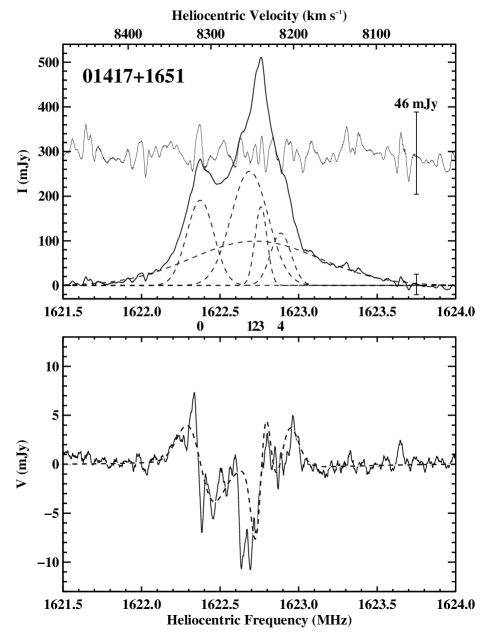
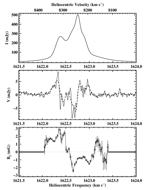
Figure 1.— Total intensity and circular polarization results for IRAS F01417$+$1651 (III Zw 35). (Top left) The Stokes $I$ spectrum (solid line; twice the conventionally defined flux density) is plotted as a function of heliocentric frequency (bottom axis) and optical heliocentric velocity (top axis). The profile of each Gaussian component is plotted as a dashed line with the corresponding component number shown below the frequency axis at the corresponding central frequency. Residuals from the composite Gaussian fit are plotted through the center of the panel (solid, light-weight line) and are expanded by a factor of 4. The scale bars near the right edge of the plot correspond to the labelled flux density range. (Bottom left) The Stokes $V$ spectrum (solid line) and its fit (dashed line). (Top right) Composite Gaussian fit to Stokes $I$. (Middle right) Measured Stokes $V$ (solid line); hypothetical Stokes $V$ (dashed line) produced by a uniform $B_{\parallel}=1$ mG using the derivative of the composite $I$ profile above. (Bottom right) Derived $B_{\parallel}$ (crosses and solid line) and uncertainty (error bars) from the $B(\nu)$ fit. All spectra and residuals are smoothed with a boxcar of 7 channels.

Table 2IRAS F10038$-$3338 (IC 2545) Gaussian Fit Parameters

	$S$	$\nu$	$\Delta\nu$	$v_{\odot}$	$B_{\parallel}$
Gaussian	(mJy)	(MHz)	(MHz)	(km s-1)	(mG)
(1)	(2)	(3)	(4)	(5)	(6)
0	$\phantom{8}47.06\pm 3.10\phantom{8}$	$1612.3870\pm 0.0044$	$0.1505\pm 0.0125$	$10221.0$	$\phantom{-}\phantom{8}1.58\pm 0.75$
1	$179.73\pm 5.15\phantom{8}$	$1612.8661\pm 0.0032$	$0.1747\pm 0.0077$	$10128.9$	$\phantom{}-1.76\pm 0.26$
2	$\phantom{8}83.85\pm 5.50\phantom{8}$	$1613.0090\pm 0.0119$	$0.9548\pm 0.0405$	$10101.4$	$-11.28\pm 1.16$
3	$227.46\pm 36.43$	$1613.0362\pm 0.0052$	$0.1222\pm 0.0095$	$10096.2$	$\phantom{}-0.07\pm 0.18$
4	$\phantom{8}\phantom{8}2.85\pm 14.04$	$1613.1570\pm 0.0089$	$0.1703\pm 0.0157$	$10073.0$	$\phantom{}-0.13\pm 0.16$
5	$\phantom{8}97.85\pm 4.75\phantom{8}$	$1613.3556\pm 0.0035$	$0.1136\pm 0.0075$	$10034.9$	$\phantom{-}\phantom{8}1.67\pm 0.33$

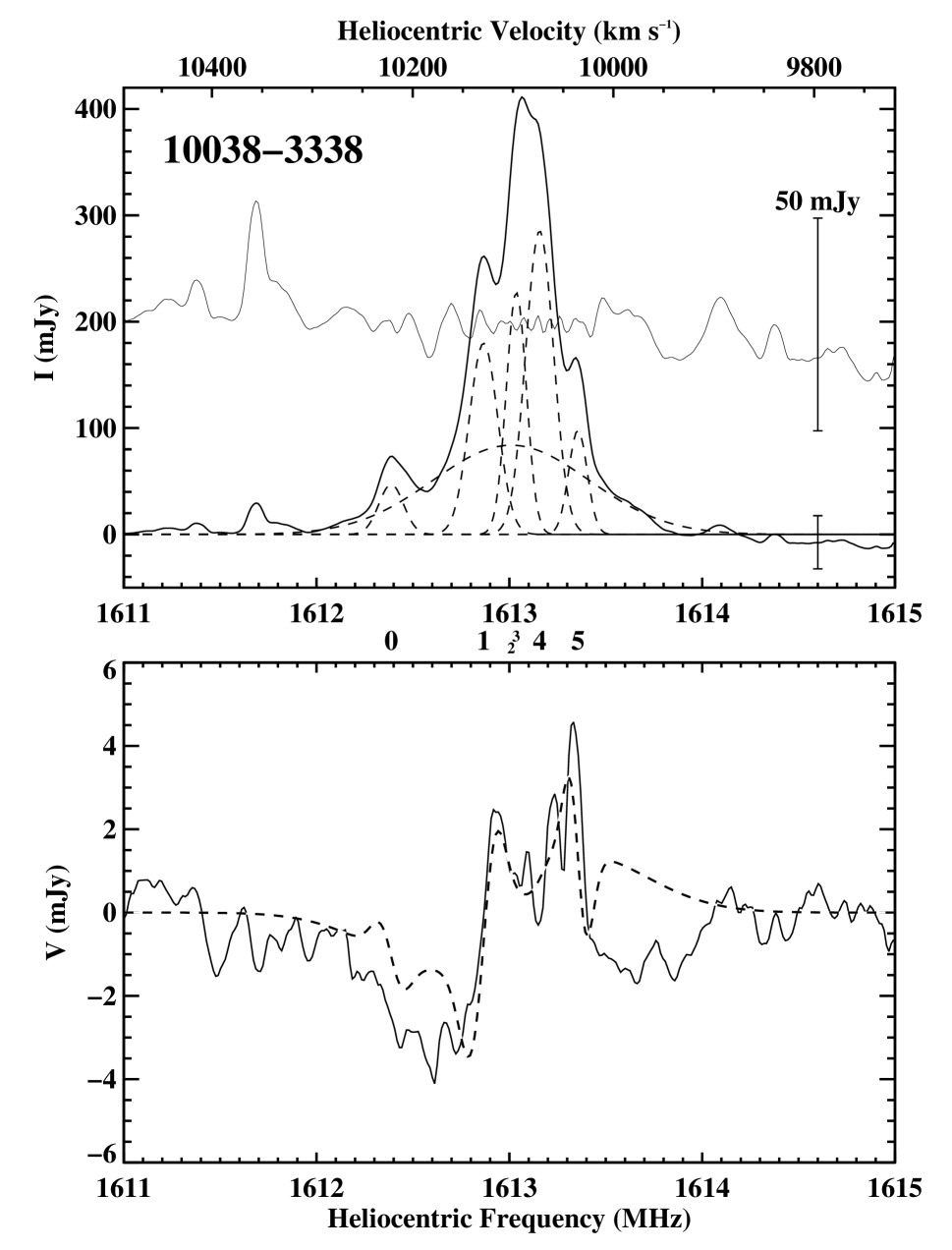
Figure 2.— Total intensity and circular polarization results for IRAS F10038$-$3338 (IC 2545). See caption for Figure 1. (Top) Residuals are expanded by a factor of 4.

Table 3IRAS F10173$+$0829 Gaussian Fit Parameters

	$S$	$\nu$	$\Delta\nu$	$v_{\odot}$	$B_{\parallel}$
Gaussian	(mJy)	(MHz)	(MHz)	(km s-1)	(mG)
(1)	(2)	(3)	(4)	(5)	(6)
0	$\phantom{8}30.62\pm 6.34$	$1589.2420\pm 0.0037$	$0.0518\pm 0.0113$	$14735.9$	$\phantom{-}2.34\pm 2.50\phantom{8}$
1	$\phantom{8}16.98\pm 5.95$	$1589.2862\pm 0.0041$	$0.0244\pm 0.0106$	$14727.1$	$\phantom{-}4.19\pm 3.42\phantom{8}$
2	$161.91\pm 7.80$	$1589.3190\pm 0.0024$	$0.1786\pm 0.0050$	$14720.7$	$\phantom{-}0.25\pm 0.89\phantom{8}$
3	$\phantom{8}15.54\pm 7.63$	$1589.3258\pm 0.0073$	$0.0463\pm 0.0240$	$14719.3$	$-2.95\pm 5.15\phantom{8}$
4	$\phantom{8}\phantom{8}0.42\pm 1.58$	$1589.5315\pm 0.0194$	$0.5661\pm 0.0257$	$14678.6$	$\phantom{-}0.93\pm 5.54\phantom{8}$
5	$\phantom{8}\phantom{8}3.50\pm 2.82$	$1589.6383\pm 0.0154$	$0.0411\pm 0.0412$	$14657.5$	$-2.90\pm 17.78$
6	$\phantom{8}16.62\pm 2.46$	$1589.8772\pm 0.0072$	$0.1670\pm 0.0279$	$14610.2$	$\phantom{-}0.80\pm 7.57\phantom{8}$

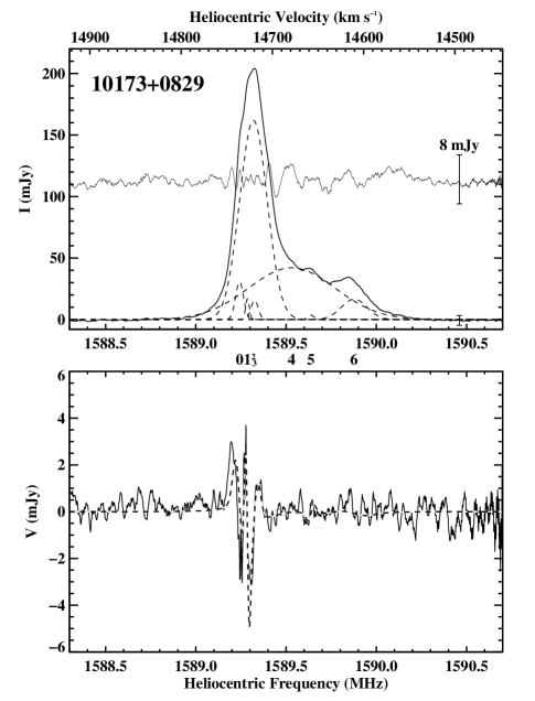
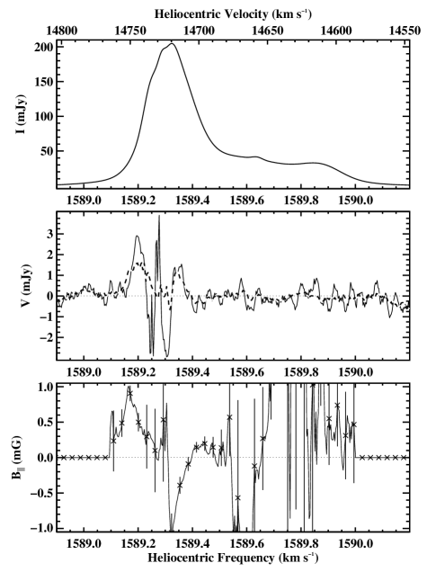
Figure 3.— Total intensity and circular polarization results for IRAS F10173$+$0829. See caption for Figure 1. (Top left) Residuals are expanded by a factor of 5. (Middle right) Dashed line shows the hypothetical Stokes $V$ produced by a uniform $B_{\parallel}=2$ mG using the derivative of the composite $I$ profile above.

Table 4IRAS F11506$-$3851 Gaussian Fit Parameters

	$S$	$\nu$	$\Delta\nu$	$v_{\odot}$	$B_{\parallel}$
Gaussian	(mJy)	(MHz)	(MHz)	(km s-1)	(mG)
(1)	(2)	(3)	(4)	(5)	(6)
0	$\phantom{8}64.73\pm 20.75$	$1650.0094\pm 0.0428$	$0.1910\pm 0.0456$	$3152.3$	$1.21\pm 0.27$
1	$102.55\pm 26.92$	$1650.1891\pm 0.0240$	$0.1810\pm 0.1018$	$3119.3$	$0.45\pm 0.20$
2	$\phantom{8}86.37\pm 83.80$	$1650.3232\pm 0.0231$	$0.1358\pm 0.0467$	$3094.7$	$0.36\pm 0.17$
3	$116.30\pm 24.97$	$1650.4685\pm 0.0257$	$0.2693\pm 0.0976$	$3068.0$	$0.73\pm 0.20$
4	$\phantom{8}\phantom{8}0.31\pm 7.25\phantom{8}$	$1650.7843\pm 0.1171$	$0.3616\pm 0.2594$	$3010.1$	$0.68\pm 0.75$
5	$\phantom{8}23.79\pm 7.46\phantom{8}$	$1651.0731\pm 0.0102$	$0.1260\pm 0.0368$	$2957.1$	$1.03\pm 0.50$

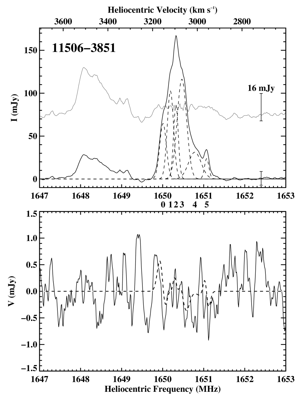
Figure 4.— Total intensity and circular polarization results for IRAS F11506$-$3851. See caption for Figure 1. (Top) Residuals are expanded by a factor of 2.

Table 5IRAS F12032$+$1707 Gaussian Fit Parameters

	$S$	$\nu$	$\Delta\nu$	$v_{\odot}$	$B_{\parallel}$
Gaussian	(mJy)	(MHz)	(MHz)	(km s-1)	(mG)
(1)	(2)	(3)	(4)	(5)	(6)
0	$\phantom{8}4.31\pm 0.54$	$1367.1002\pm 0.0169$	$0.4082\pm 0.0370$	$65844.0$	$\phantom{}-6.79\pm 7.94\phantom{8}$
1	$\phantom{8}3.95\pm 0.96$	$1367.6739\pm 0.0457$	$0.7915\pm 0.1793$	$65690.6$	$\phantom{-}30.42\pm 12.43$
2	$\phantom{8}8.42\pm 0.99$	$1368.8016\pm 0.0094$	$0.6264\pm 0.0448$	$65389.5$	$\phantom{-}\phantom{8}6.91\pm 4.86\phantom{8}$
3	$\phantom{8}3.00\pm 0.34$	$1369.5922\pm 0.0071$	$0.1460\pm 0.0207$	$65178.7$	$\phantom{}-1.05\pm 6.48\phantom{8}$
4	$\phantom{8}0.21\pm 0.36$	$1369.6903\pm 0.0452$	$2.6434\pm 0.1574$	$65152.6$	$\phantom{}-3.25\pm 3.98\phantom{8}$
5	$\phantom{8}3.23\pm 0.54$	$1369.9216\pm 0.0036$	$0.0450\pm 0.0089$	$65091.0$	$\phantom{-}\phantom{8}3.10\pm 3.41\phantom{8}$
6	$\phantom{8}6.67\pm 0.34$	$1370.7194\pm 0.0064$	$0.2954\pm 0.0165$	$64878.6$	$\phantom{-}11.64\pm 4.31\phantom{8}$
7	$21.67\pm 0.65$	$1371.2516\pm 0.0030$	$0.4769\pm 0.0115$	$64737.0$	$\phantom{-}10.90\pm 1.72\phantom{8}$
8	$16.99\pm 0.46$	$1371.3316\pm 0.0010$	$0.0849\pm 0.0029$	$64715.8$	$\phantom{-}17.92\pm 0.89\phantom{8}$
9	$16.19\pm 3.38$	$1372.1576\pm 0.0568$	$0.4872\pm 0.0531$	$64496.4$	$\phantom{-}\phantom{8}1.78\pm 2.48\phantom{8}$
10	$25.02\pm 4.51$	$1372.3299\pm 0.0027$	$0.2795\pm 0.0165$	$64450.6$	$\phantom{}-1.45\pm 1.12\phantom{8}$
11	$\phantom{8}9.56\pm 0.51$	$1372.7780\pm 0.0412$	$0.7315\pm 0.0588$	$64331.7$	$-11.69\pm 4.98\phantom{8}$
12	$\phantom{8}2.02\pm 0.21$	$1373.8371\pm 0.0179$	$0.3807\pm 0.0500$	$64051.0$	$\phantom{-}20.61\pm 15.49$

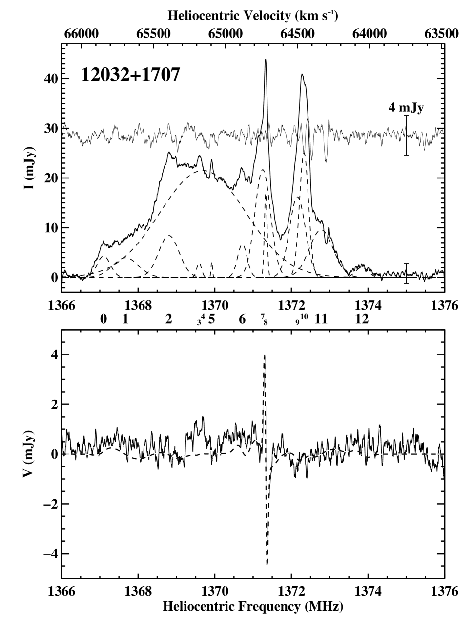
Figure 5.— Total intensity and circular polarization results for IRAS F12032$+$1707. See caption for Figure 1. (Top) Residuals are expanded by a factor of 2.

Table 6IRAS F12112$+$0305 Gaussian Fit Parameters

	$S$	$\nu$	$\Delta\nu$	$v_{\odot}$	$B_{\parallel}$
Gaussian	(mJy)	(MHz)	(MHz)	(km s-1)	(mG)
(1)	(2)	(3)	(4)	(5)	(6)
0	$16.19\pm 0.75$	$1554.1822\pm 0.0013$	$0.1467\pm 0.0054$	$21831.1$	$-0.20\pm 1.99$
1	$58.16\pm 0.51$	$1554.2767\pm 0.0048$	$0.5188\pm 0.0098$	$21811.6$	$\phantom{-}0.25\pm 1.17$
2	$48.63\pm 0.97$	$1554.5634\pm 0.0007$	$0.1893\pm 0.0028$	$21752.3$	$\phantom{-}1.02\pm 0.77$
3	$13.83\pm 0.59$	$1554.5641\pm 0.0006$	$0.0309\pm 0.0017$	$21752.1$	$\phantom{-}0.27\pm 1.03$
4	$\phantom{8}0.32\pm 0.34$	$1554.8544\pm 0.0037$	$0.4359\pm 0.0063$	$21692.1$	$\phantom{-}3.09\pm 1.92$

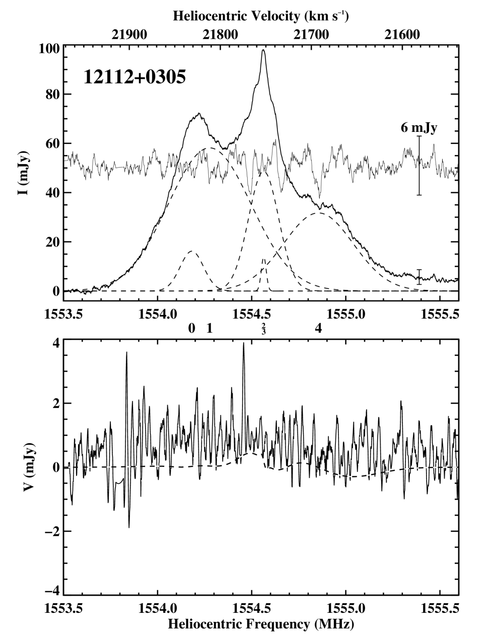
Figure 6.— Total intensity and circular polarization results for IRAS F12112$+$0305. See caption for Figure 1. (Top) Residuals are expanded by a factor of 4.

Table 7IRAS F14070$+$0525 Gaussian Fit Parameters

	$S$	$\nu$	$\Delta\nu$	$v_{\odot}$	$B_{\parallel}$
Gaussian	(mJy)	(MHz)	(MHz)	(km s-1)	(mG)
(1)	(2)	(3)	(4)	(5)	(6)
0	$\phantom{8}3.50\pm 0.22$	$1315.2359\pm 0.0105$	$0.4088\pm 0.0317$	$80262.3$	$-10.42\pm 10.49$
1	$\phantom{8}8.95\pm 0.19$	$1316.0759\pm 0.0715$	$2.1625\pm 0.0861$	$80019.7$	$\phantom{-}26.65\pm 9.57\phantom{8}$
2	$\phantom{8}5.70\pm 0.30$	$1316.2886\pm 0.0047$	$0.2040\pm 0.0134$	$79958.4$	$\phantom{-}\phantom{8}1.76\pm 4.65\phantom{8}$
3	$11.26\pm 0.68$	$1316.9061\pm 0.0100$	$0.6771\pm 0.0302$	$79780.3$	$\phantom{}-3.31\pm 4.67\phantom{8}$
4	$\phantom{8}0.08\pm 0.50$	$1317.5519\pm 0.0118$	$0.4878\pm 0.0271$	$79594.2$	$\phantom{}-3.16\pm 5.59\phantom{8}$
5	$\phantom{8}2.78\pm 0.26$	$1318.8802\pm 0.0106$	$0.2664\pm 0.0307$	$79212.1$	$\phantom{-}12.72\pm 10.82$
6	$10.76\pm 0.16$	$1319.1605\pm 0.0113$	$1.2737\pm 0.0199$	$79131.6$	$-12.92\pm 6.16\phantom{8}$

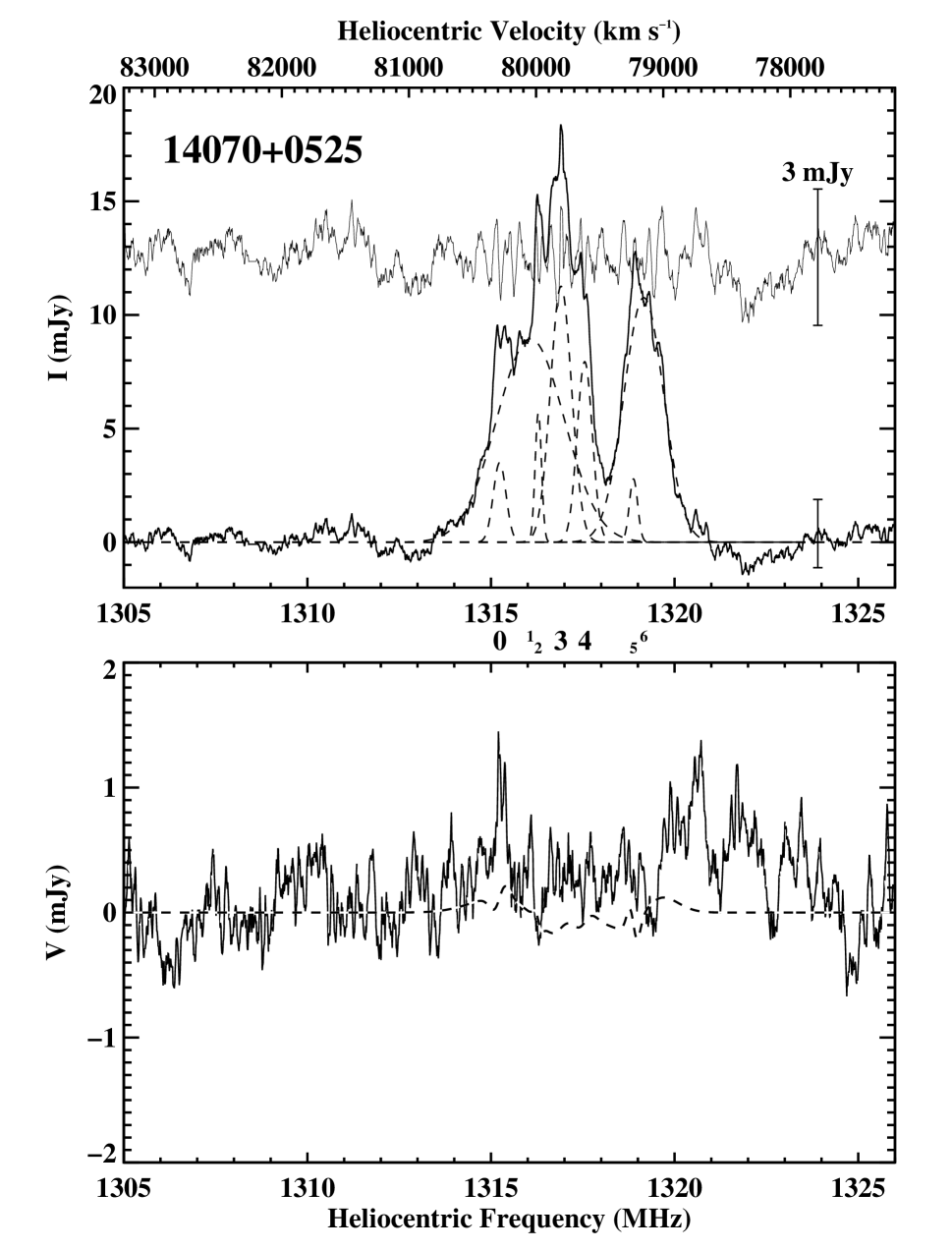
Figure 7.— Total intensity and circular polarization results for IRAS F14070$+$0525. See caption for Figure 1. (Top) Residuals are expanded by a factor of 2.

Table 8IRAS F15327$+$2340 (Arp 220) Gaussian Fit Parameters

	$S$	$\nu$	$\Delta\nu$	$v_{\odot}$	$B_{\parallel}$
Gaussian	(mJy)	(MHz)	(MHz)	(km s-1)	(mG)
(1)	(2)	(3)	(4)	(5)	(6)
0	$\phantom{8}14.52\pm 0.98$	$1637.1424\pm 0.0008$	$0.0243\pm 0.0020$	$5533.2$	$-4.78\pm 0.53$
1	$\phantom{8}10.92\pm 0.61$	$1637.3105\pm 0.0018$	$0.0709\pm 0.0050$	$5501.9$	$-0.11\pm 1.21$
2	$\phantom{8}11.80\pm 1.02$	$1637.5074\pm 0.0009$	$0.0231\pm 0.0024$	$5465.2$	$-2.78\pm 0.64$
3	$\phantom{8}10.12\pm 1.00$	$1637.5736\pm 0.0011$	$0.0241\pm 0.0029$	$5452.9$	$\phantom{-}7.77\pm 0.76$
4	$\phantom{8}\phantom{8}0.90\pm 0.77$	$1637.7198\pm 0.0002$	$0.0590\pm 0.0006$	$5425.6$	$-2.78\pm 0.13$
5	$\phantom{8}51.49\pm 1.06$	$1637.8723\pm 0.0005$	$0.0621\pm 0.0016$	$5397.2$	$\phantom{-}0.33\pm 0.25$
6	$324.77\pm 3.96$	$1637.8916\pm 0.0010$	$0.3362\pm 0.0028$	$5393.6$	$\phantom{-}0.26\pm 0.12$
7	$\phantom{8}97.84\pm 2.60$	$1638.0196\pm 0.0008$	$0.0800\pm 0.0023$	$5369.7$	$-0.15\pm 0.18$
8	$293.07\pm 4.06$	$1638.0313\pm 0.0011$	$1.0064\pm 0.0075$	$5367.6$	$\phantom{-}0.14\pm 0.21$
9	$386.20\pm 5.88$	$1638.1189\pm 0.0007$	$0.0882\pm 0.0012$	$5351.2$	$-0.76\pm 0.06$
10	$\phantom{8}81.13\pm 2.84$	$1638.1375\pm 0.0002$	$0.0292\pm 0.0008$	$5347.8$	$-0.24\pm 0.11$
11	$237.99\pm 4.75$	$1638.2098\pm 0.0011$	$0.1039\pm 0.0024$	$5334.3$	$\phantom{-}0.66\pm 0.10$
12	$\phantom{8}46.95\pm 2.66$	$1638.3468\pm 0.0051$	$0.1894\pm 0.0103$	$5308.8$	$-1.03\pm 0.59$
13	$\phantom{8}18.22\pm 1.02$	$1638.4199\pm 0.0008$	$0.0342\pm 0.0024$	$5295.2$	$\phantom{-}0.20\pm 0.50$
14	$\phantom{8}19.79\pm 0.78$	$1638.6066\pm 0.0011$	$0.0769\pm 0.0036$	$5260.4$	$\phantom{-}0.22\pm 0.69$
15	$\phantom{8}\phantom{8}7.62\pm 0.60$	$1638.8445\pm 0.0033$	$0.1038\pm 0.0103$	$5216.1$	$\phantom{-}1.78\pm 2.10$
16	$\phantom{8}11.23\pm 0.82$	$1638.9714\pm 0.0014$	$0.0367\pm 0.0034$	$5192.5$	$\phantom{-}1.42\pm 0.86$
17	$\phantom{8}13.18\pm 0.57$	$1639.0663\pm 0.0018$	$0.0908\pm 0.0051$	$5174.9$	$-0.46\pm 1.15$

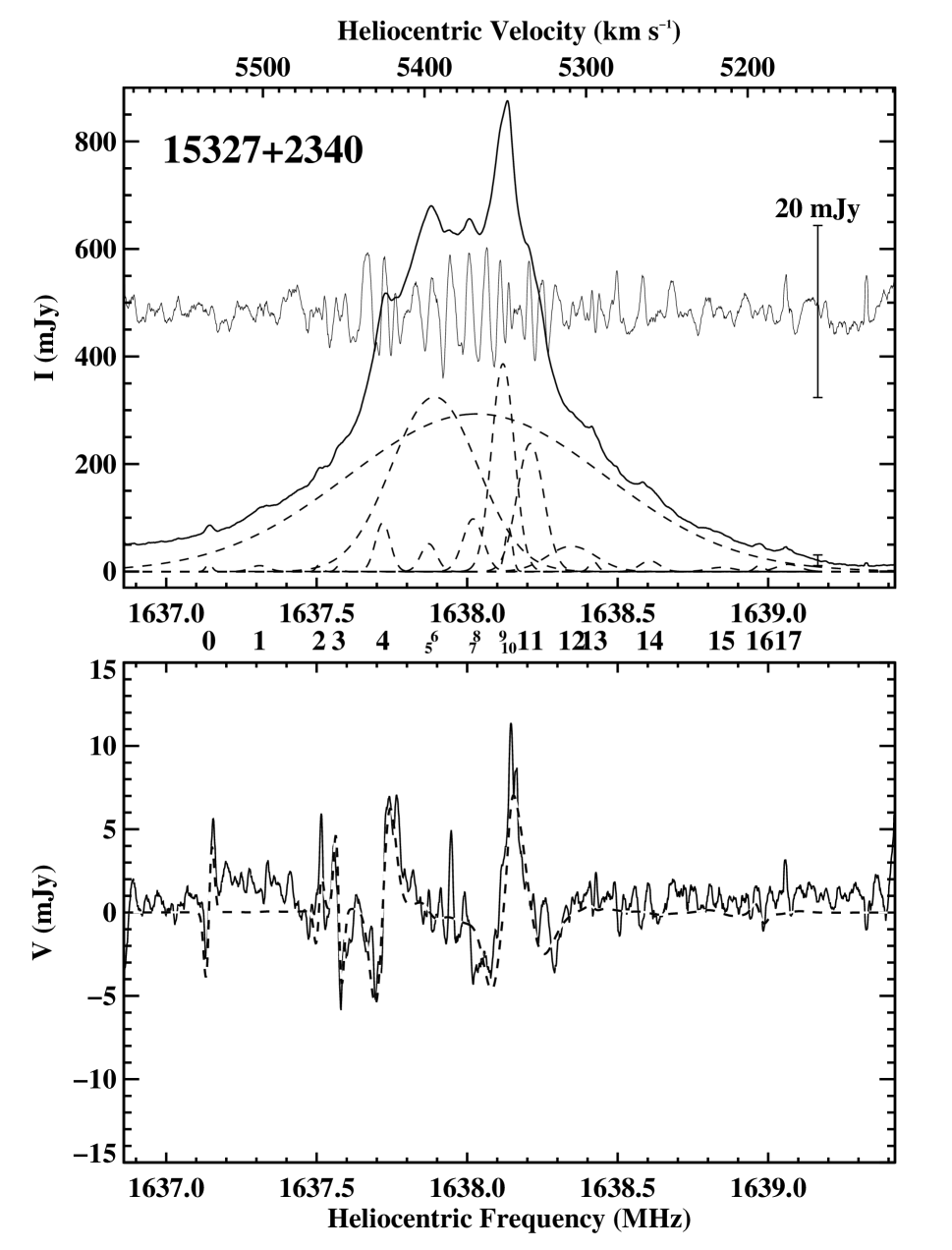
Figure 8.— Total intensity and circular polarization results for IRAS F15327$+$2340 (Arp 220). See caption for Figure 1. (Top) Residuals are expanded by a factor of 16.

Figure 9.— Linear polarization results for IRAS F01417$+$1651 (III Zw 35). (Left) Top panel shows Stokes $I$, middle panel shows the linearly polarized intensity, and bottom panel shows the position angle over the entire 12.5 MHz bandwidth. (Right) Same as left panels, but with the frequency range narrowed to 6 MHz; the bottom right plot also shows the fitted Faraday rotation as a dashed line whose slope was determined by fitting to the points marked as diamonds. All spectra are plotted as a function of heliocentric frequency (bottom axis). The top panels show the optical heliocentric velocity (top axis). All spectra are smoothed by a boxcar of 23 channels.

Figure 10.— Linear polarization results for IRAS F10173$+$0829. See caption for Figure 9. All spectra are smoothed by a boxcar of 17 channels.

Figure 11.— Linear polarization results for IRAS F12032$+$1707. See caption for Figure 9. All spectra are smoothed by a boxcar of 31 channels.

Figure 12.— Linear polarization results for IRAS F12112$+$0305. See caption for Figure 9. All spectra are smoothed by a boxcar of 11 channels.

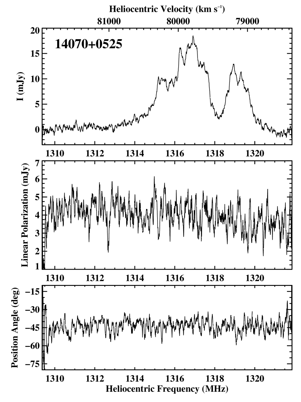
Figure 13.— Linear polarization results for IRAS F14070$+$0525. See caption for Figure 9. All spectra are smoothed by a boxcar of 11 channels.

Figure 14.— Linear polarization results for IRAS F15327$+$2340 (Arp 220). See caption for Figure 9. (Right) The frequency range has been narrowed to 4 MHz. All spectra are smoothed by a boxcar of 9 channels.