The Flux Auto- and Cross-Correlation of the Ly$\alpha$ Forest.
II. Modelling Anisotropies with Cosmological Hydrodynamic Simulations

Abstract

The isotropy of the Ly$\alpha$forest in real-space uniquely provides a measurement of cosmic geometry at $z>2$. The angular diameter distance for which the correlation function along the line of sight and in the transverse direction agree corresponds to the correct cosmological model. However, the Ly$\alpha$ forest is observed in redshift-space where distortions due to Hubble expansion, bulk flows, and thermal broadening introduce anisotropy. Similarly, a spectrograph’s line spread function affects the autocorrelation and cross-correlation differently. In this the second paper of a series on using the Ly$\alpha$ forest observed in pairs of QSOs for a new application of the Alcock-Paczyński (AP) test, these anisotropies and related sources of potential systematic error are investigated with cosmological hydrodynamic simulations. Three prescriptions for galactic outflow were compared and found to have only a marginal effect on the Ly$\alpha$ flux correlation (which changed by at most 7% with use of the currently favored variable-momentum wind model vs. no winds at all). An approximate solution for obtaining the zero-lag cross-correlation corresponding to arbitrary spectral resolution directly from the zero-lag cross-correlation computed at full-resolution (good to within 2% at the scales of interest) is presented. Uncertainty in the observationally determined mean flux decrement of the Ly$\alpha$ forest was found to be the dominant source of systematic error; however, this is reduced significantly when considering correlation ratios. We describe a simple scheme for implementing our results, while mitigating systematic errors, in the context of a future application of the AP test.

1. Introduction

Significant observational and theoretical advances in recent decades have made the Ly$\alpha$ forest a powerful and unique cosmological tool for studying the high-redshift universe. Originally named (Weymann et al., 1981) for the dense pattern of seemingly discrete Ly$\alpha$ absorption lines seen in high-redshift QSO spectra (Lynds, 1971), the absorption is now understood to trace a continuous distribution of non-uniform neutral hydrogen gas that in turn maps the underlying dark matter (see Rauch 1998 for a review). The competing processes of recombination and photoionization lead to a tight relationship between the density of the gas and the neutral fraction, giving rise to a relatively straightforward link between Ly$\alpha$ absorption and the large scale structure of the universe. Cosmological simulations employing this prescription have had remarkable success reproducing detailed properties of the Ly$\alpha$ forest provided by high-resolution ground-based QSO spectra (Cen et al., 1994; Zhang et al., 1995; Hernquist et al., 1996; Theuns et al., 1998) and low-$z$ HST observations (Petitjean et al., 1995; Davé et al., 1999), paving the way for the Ly$\alpha$ forest to be reliably used for cosmological investigation.

Hui et al. (1999) and McDonald & Miralda-Escudé (1999) first suggested using autocorrelation and cross-correlation measurements in the Ly$\alpha$ forest for a new application of the Alcock-Paczyński (AP) test (Alcock & Paczynski, 1979), a purely geometric method for measuring cosmological parameters that is primarily sensitive to $\Omega_{\Lambda}$ at $z>1$. The essence of this cosmological test is that spherical objects observed at high redshift will only appear to be equal in their radial and transverse extent if the correct angular diameter distance is used to determine the latter. More generally, the correlation function of an isotropic medium, such as the Ly$\alpha$ forest, measured as a function of separation along the line of sight (the autocorrelation $\xi_{\parallel}$) and in the transverse direction (the cross-correlation $\xi_{\perp}$) will agree only if the correct cosmology is assumed.

Spectroscopy of the Ly$\alpha$ forest in any single QSO spectrum yields the complete autocorrelation, albeit with significant variance from one line of sight to another. The cross-correlation, on the other hand, must be pieced together from pairs of QSOs with different transverse separations. Until recently, only approximately a dozen pairs with similar redshifts (so that their Ly$\alpha$ forests overlap) and separations of a few arcminutes or less (the correlation signal diminishes rapidly beyond this point) were known (see, e.g., Rollinde et al. 2003 and references therein). The 2dF QSO Redshift Survey (2QZ; Croom et al., 2004) significantly increased this number, and with motivation from McDonald (2003), moderate resolution spectra (FWHM $\simeq$ 2.5 Å) with modest signal-to-noise ratios (S/N $>$ 10 per pixel) have been obtained for more than 50 of these pairs at the VLT (Coppolani et al., 2006), MMT, and Magellan (Marble et al., 2008, hereafter referred to as Paper I) observatories.

While conceptually simple, the Ly$\alpha$ forest variant of the AP test is not as straightforward as measuring the autocorrelation and cross-correlation from pairs of QSOs and determining the angular diameter distance which satisfies the presumption of isotropy. Rather, two additional sources of anisotropy must be accounted for. First, the line spread function (LSF) of the spectrograph smooths QSO spectra along the line of sight, affecting the autocorrelation and cross-correlation differently. Second, nonzero velocities caused by the expansion of the universe, gravitational collapse, and thermal broadening make the correlation function in redshift-space ($z$-space) anisotropic (Kaiser, 1987). Fortunately, the theoretical work of Hui et al. (1999), McDonald & Miralda-Escudé (1999), and McDonald (2003) found that these redshift-space distortions can be disentangled from the desired cosmological signature.

The aim of this paper is to investigate these non-cosmological anisotropies in the Ly$\alpha$ flux correlation function in a manner which is directly applicable to observations of QSO pairs that are suitable for a new application of the AP test. To this end we have employed a variety of cosmological hydrodynamic simulations to model the autocorrelation and cross-correlation of the Ly$\alpha$ forest in both redshift-space and real-space. These simulations are described in § 2, as well as our procedure for extracting mock Ly$\alpha$ absorption spectra from them. In § 3 and § 3.1 we introduce the correlation function and discuss how to mitigate relevant size and mass resolution limitations of the current generation of simulations. The effect of arbitrary spectral resolution on the correlation function is the subject of § 3.2. Additional potential sources of systematic error, both computational and observational, are addressed in § 4. The implications of our results for the AP test are the topic of § 5. Finally, in § 6, we summarize this work and its findings.

2. Simulation Data

2.1. Simulations

This body of work draws from a suite of eight cosmological simulations which primarily differ in their size, mass resolution, and prescription for galactic outflow (Table 1). Together, w16n256vzw (abbreviated as wvzw) and g6 mitigate the effects of limitations in volume and mass resolution as discussed in § 3.1. Differing wind models (described in § 4.5) are investigated with the w16n256cw and w16n256nw simulations (abbreviated as wcw and wnw respectively), which are otherwise identical to wvzw. Similarly, the q1-q4 simulations differ only by their number of particles, $N_{p}$, and are used in § 3.1 to test for convergence as a function of mass resolution. All of these simulations have been the subject of previous study; therefore, we address only the relevant details and direct interested readers to the references provided for additional discussion. The common genesis of these simulations is described below, while their differences are contrasted in Table 1 and the sections referenced above.

The $N$-body $+$ hydrodynamic code Gadget (Springel et al., 2001), with modifications described in Springel & Hernquist (2003), was used to create q1, q2, q3, q4, and g6 (Springel & Hernquist, 2003, but also see Finlator et al. (2006) regarding g6), while wvzw, wcw, and wnw (Oppenheimer & Davé, 2006) were run with a similarly modified version of its successor Gadget-2 (Springel, 2005). This code computes gravitational forces via a tree particle-mesh solver and hydrodynamical forces with an entropy-conservative formulation of smoothed particle hydrodynamics (SPH). Modelling of additional physical processes includes prescriptions for star formation and supernova feedback within evolving galaxies, which impact the intergalactic medium (IGM) via outflow from galactic winds. A spatially uniform photoionization background is included, with the spectral shape and redshift evolution given by Haardt & Madau (1996) and Haardt & Madau (2001) for the Gadget and Gadget-2 runs respectively. Radiative heating and cooling is calculated assuming photoionization equilibrium and optically thin gas. All of the simulations were run as cubic volumes with periodic boundary conditions and the same cosmological parameters ($\Omega_{m}=0.3$, $\Omega_{\Lambda}=0.7$, $\Omega_{b}=0.04$, $\sigma_{8}=0.9$, and $h=0.7$), which we assume throughout this paper.

2.2. Line of Sight Selection

“Observed” lines of sight through the simulation box (parallel to the three principal axes) were grouped into sets, each of which probed the desired separation range ($0-5$ arcminutes). $N_{s}$ sets were randomly distributed across each of the three mutually orthogonal faces of the box in order to representatively sample the diversity of structure present in the simulation volume. The value of $N_{s}$ (Table 1), which roughly scales inversely with the box length of the simulation cube for comparable total path length, yields oversampled structure (correlated measurements) in some cases. However, there are sufficient independent lines of sight through each simulation to achieve negligible uncertainty in the Ly$\alpha$ forest flux correlation mean despite considerable variance.

The lines of sight in a given set were arranged in the following manner. A position on the face of the simulation box was randomly selected, from which an imaginary $300\arcsec$ long line was extended at a random angle within the same plane. If the line happened to intersect an edge of the simulation face, it was continued on the opposite side, per the wrapped boundary conditions. The two opposing ends of the line and 11 intermediate positions (2, 3, 8, 12, 15, 25, 45, 80, 150, 210, and 250 arcseconds from the origin) defined starting coordinates for that set. The intervals between these 13 lines of sight, determined via a Monte Carlo approach designed to maximize sampling of angular separation (particularly at small separations where the correlation function evolves more rapidly) with a minimal number of spectra, yield 73 pairings with unique separations.

2.3. Ly$\alpha$ Flux Spectra

Two Ly$\alpha$ transmitted flux spectra, one corresponding to redshift-space and another to real-space, were computed as a function of position, $x$, along each line of sight using a modified version of the program specexbin (originally part of tipsy; Davé et al., 1999). First, the physical properties of the gas (density, temperature, and velocity) were calculated at $\simeq 20~{}h^{\textrm{-}1}$ comoving kpc intervals ($\Delta v\,\simeq\,2.1\,$km s${}^{\textrm{-}1}$ or $\Delta\lambda\,\simeq\,0.029\,$Å at $z=2.4$). For the real-space spectra, the velocities (resulting from Hubble expansion across the length of the box, bulk flows, and thermal broadening) were reset to zero. Then, the corresponding H I opacities, $\tau$, were determined, using ionization fraction lookup tables generated with Cloudy v96 (Ferland et al., 1998), and converted to Ly$\alpha$ transmitted flux,

$$f(x)=e^{-\tau(x)}.$$ (1)

In an additional intermediate step, the extracted opacities were multiplied by a single scaling factor in order to match the mean transmitted flux, $\langle f\rangle$, in redshift-space to the observed value of either Press et al. (1993) or Kirkman et al. (2005). For the moderately overdense regions characteristic of the Ly$\alpha$ forest ($\rho/\bar{\rho}<10$), this has the same effect as changing the amplitude of the photoionizing background (which determines $\langle f\rangle$) when running the simulation and/or when later computing the ionization fraction to determine opacity (Croft et al., 1998). The appropriate scaling was determined for each simulation and redshift via an iterative process. The raw opacity values from all redshift-space extractions were multiplied by a single scaling factor (originally one), converted to fluxes, and averaged. The scaling factor was then adjusted to be higher or lower as needed, and these steps were repeated with incrementally smaller adjustments until the resulting mean flux agreed with the desired value. This convergence was considered complete when the difference was less than or equal to the formal error in the calculated mean. Given the large number of extracted opacities, this typically corresponded to a relative difference of less than 0.01%.

Figure 1 shows the resulting spectrum for a single line of sight through the wvzw simulation box at different redshifts. The corresponding set of lines of sight (for $z=3$) is shown in Figure 2, illustrating the decreasing correlation (in the form of visual similarity) at increasingly larger transverse separations. A comparison of the same line of sight in real-space and redshift-space is provided in Figure 3, where the redistribution of opacity due to redshift-space distortions is subtle, but evident. In addition, narrower absorption features can be seen relative to a different line of sight through the larger g6 simulation, due to the poorer mass resolution of the latter.

3. The Correlation Function

From the ensemble of lines of sight through each simulation, we know the transmitted Ly$\alpha$ flux as a function of velocity,

$$v\equiv\frac{H(z_{sim})\,x}{1+z_{sim}},$$ (2)

in the radial ($v_{\parallel}$) and transverse ($v_{\perp}$) directions for $\Sigma n=N_{s}$ different realizations (i.e., sets of lines of sight). Here $H(z_{sim})$ is the value of the Hubble parameter at the fixed redshift of the simulation, and the denominator accounts for $x$ being in comoving coordinates. For notational convenience, we define $\delta$ to be the relative difference between $f$ and the global mean,

$$\delta_{n}\left(v_{\parallel},v_{\perp}\right)\equiv\frac{f_{n}\left(v_{\parallel},v_{\perp}\right)}{\langle f\rangle}-1.$$ (3)

The relation between transmitted flux separated along the line of sight or in the transverse direction by a velocity difference $\Delta v$ is given by the autocorrelation,

$$\xi_{\parallel}(\Delta v)=\frac{1}{N_{s}}\sum_{n=1}^{N_{s}}\frac{1}{N_{\perp}}\sum_{i=1}^{N_{\perp}}\frac{1}{N_{\parallel}}\sum_{j=1}^{N_{\parallel}}\delta_{n}\left(v_{\parallel_{j}},v_{\perp_{i}}\right)\,\delta_{n}\left(v_{\parallel_{j}}+\Delta v,v_{\perp_{i}}\right),$$ (4)

and zero-lag cross-correlation,

$$\xi_{\perp}\!\left(\Delta v\right)=\frac{1}{N_{s}}\sum_{n=1}^{N_{s}}\frac{1}{N_{\parallel}}\sum_{j=1}^{N_{\parallel}}\delta_{n}\left(v_{\parallel_{j}},v_{\perp_{i}}\right)\,\delta_{n}\left(v_{\parallel_{j}},v_{\perp_{i}}+\Delta v\right),$$ (5)

respectively. Note that $f_{n}$ (and therefore $\delta_{n}$) is periodic due to the wrapped boundary conditions of the simulation box. In real-space, the correlation of the Ly$\alpha$ forest is isotropic, and $\xi_{\parallel}=\xi_{\perp}$. Figure 4 confirms this basic result for the hybrid correlation measurements (discussed in § 3.1) at $z=3$ and shows the anisotropy introduced in redshift-space.

3.1. Box Length vs. Mass Resolution

The Ly$\alpha$ forest is believed to have formed, via gravitational collapse, from perturbations in the initial density field. In order to reliably model the correlation function of the Ly$\alpha$ forest, simulations must evolve a sufficiently large volume with adequate mass resolution. A simulation box length that is too small, or a gas particle mass that is too large, excludes relevant perturbations on large and small scales respectively. In the moderately overdense regime of the Ly$\alpha$ forest, growth is sufficiently non-linear that perturbations of different sizes become coupled, and the correlation function is affected even at scales not excluded. In addition, aliasing due to the periodic boundary conditions of the simulations is extended from half the box length ($L$) to smaller scales (we limit our analysis to separations less than $L/3-L/4$). Since simulations which can satisfy both of these competing demands are not yet available, we mitigate these effects by forming hybrid correlation curves from two different simulations which meet the requirements independently.

The wvzw simulation has $256^{3}$ gas particles within an $L=16~{}h^{\textrm{-}1}$ Mpc box, yielding a gas particle mass of $m_{gas}=2.71\times 10^{6}~{}h^{\textrm{-}1}~{}M_{\sun}$. In order to verify that this mass resolution is sufficient for our purposes, we used the q1, q2, q3, and q4 simulations to test for convergence (note that the result may be simulation code dependent). The q-series are identical except for particle number, with gas particle masses which decrease with increasing series number (42.4, 12.5, 3.72, and 1.10 in units of $10^{6}~{}h^{\textrm{-}1}~{}M_{\sun}$). As a consequence of their small box length ($L=10~{}h^{\textrm{-}1}$ Mpc), the correlation is artificially depressed and the autocorrelation crosses zero on the scales of interest to us. Therefore, in order to make meaningful comparisons (avoiding division by zero), the q-series correlation curves were all increased by an equal, constant amount such that q1 agrees with g6 (which has a comparable gas mass resolution, but a much larger box length) at 445 km s${}^{\textrm{-}1}$ (this velocity choice is motivated below).

As shown in the left panels of Figure 5, the cross-correlation (top) and autocorrelation (bottom) from q3 agree well with q4 ($<3\%$ relative difference for $\Delta v$ corresponding to less than $L/4$). We conclude that wvzw, which has a smaller gas particle mass than q3, is not significantly compromised by mass resolution. However, in addition to missing large scale power due to the $L=16~{}h^{\textrm{-}1}$ Mpc box length, the reliable separation range ($\scriptstyle\lesssim$ $L/4$) probed by wvzw corresponds to only $394-444$ km s${}^{\textrm{-}1}$ at $z=2-3$. Conversely, the box length of the larger ($L=100~{}h^{\textrm{-}1}$ Mpc), but much lower-resolution ($484^{3}$ gas particles, $m_{gas}=9.79\times 10^{7}~{}h^{\textrm{-}1}~{}M_{\sun}$), g6 simulation should more than suffice. McDonald (2003) found little difference in the correlation function between $L=40$ and $80~{}h^{\textrm{-}1}$ Mpc simulations.

In Figure 6, we consider the subtracted difference between the correlation functions of wcw and g6 (solid lines) in order to characterize the effects of insufficient simulation volume and mass resolution and to motivate a methodology for forming hybrid correlation curves that mitigate them. Note that wcw is used in lieu of wvzw in order to elliminate any additional differences due to wind models. The signature of poor mass resolution is illustrated (dotted lines in Fig. 6) by the correlation difference between q1 and the mean of q3 and q4 (which closely corresponds to the mass resolution of wcw). The nature of the suppression of wcw due to its small box length is then reflected in the residual (dash-dotted lines in Fig. 6) between these two curves. However, since the mass resolution of q1 is superior to g6 by more than a factor of 2, the dotted line underestimates the effect for g6. Extrapolation from the right panels of Figure 5 is poorly constrained, although accounting for the trend implies significant flattening of the dash-dotted line (Figure 6) on small scales. Such a relatively smooth alteration of the correlation function due to insufficient box length is consistent with the expectation of constant suppression when the evolution of coupled modes is not accounted for (McDonald et al., 2000, see Figure 15). Although the true effect is likely not a constant offset at all scales, this appears to be a reasonable approximation. Note also that the disparity between wcw and g6 at sufficiently large $\Delta v$ appears to be purely a box length effect. Therefore, we define the hybrid correlation function $\xi^{h}$ to be equal to $\xi^{g6}$ for $\Delta v$ greater than an adopted splice velocity, $v_{s}$. For $\Delta v<v_{s}$, $\xi_{\parallel}^{h}$ is equal to $\xi_{\parallel}^{wvzw}$ plus the difference between $\xi_{\parallel}^{g6}$ and $\xi_{\parallel}^{wvzw}$ at the splice velocity. In the case of the cross-correlation, this is slightly modified to preserve the boundary condition $\xi_{\perp}\left(0\right)=\xi_{\parallel}\left(0\right)$. More explicitly,

$$\begin{array}[]{rcl}\xi^{h}\left(\Delta v>v_{s}\right)&=&\xi^{g6}\left(\Delta v\right)\\ \xi_{\parallel}^{h}\left(\Delta v<v_{s}\right)&=&\xi_{\parallel}^{wvzw}\left(\Delta v\right)+\tilde{\delta}_{\parallel}\\ \xi_{\perp}^{h}\left(\Delta v<v_{s}\right)&=&\xi_{\perp}^{wvzw}\left(\Delta v\right)+\tilde{\delta}_{\perp}+\left(\frac{\delta_{\perp}-\delta_{\parallel}}{v_{s}}\right)\Delta v\\ \tilde{\delta}&\equiv&\xi^{g6}\left(v_{s}\right)-\xi^{wvzw}\left(v_{s}\right).\par\end{array}$$ (6)

The value of $v_{s}$ was chosen to be the minimum velocity at which the effect of the g6 mass resolution can be assumed to be negligible. In order to ensure isotropy in real-space, $v_{s}$ must be the same for the autocorrelation and cross-correlation. Thus, based on Figures 5 and 6, 445 km s${}^{\textrm{-}1}$ was adopted as the splice velocity (for all redshifts). It is worth noting that the resulting hybrid correlation curves are insensitive to the exact choice of $v_{s}$ due to the relative flatness of the difference between $\xi^{g6}$ and $\xi^{wvzw}$ on these scales.

3.2. Accounting For Spectral Resolution

A real spectrum (i.e., observed with a telescope) is a convolution, $\mathcal{S_{\parallel}}$, of the true transmitted flux along the line of sight with the LSF of the spectrograph. The LSF is generally Gaussian, and the width, $\sigma$, determines the resolution of the data,

$$\mathcal{S_{\parallel}}\left[\tilde{f}\left(v_{\parallel_{j}}\right),\sigma\right]\equiv\sum_{k=j-\alpha}^{j+\alpha}\tilde{f}\left(v_{\parallel_{k}}\right)\,\frac{1}{\sqrt{2\pi}\,\sigma}\,\,e^{\frac{-(v_{\parallel_{j}}-v_{\parallel_{k}})^{2}}{2\,\sigma^{2}}},$$ (7)

where $\alpha$ must be sufficiently large with respect to $\sigma$ that the tails of the exponential are effectively zero at the limits of convolution. Figure 3 provides a comparison of a simulated spectrum at full-resolution and the same spectrum degraded to FWHM $=2\sqrt{2\ln 2}$ and $\sigma=\ 2.5\,$Å. Similar to the anistropy introduced by redshift-space distortions, this smoothing along the line of sight changes the autocorrelation differently than the cross-correlation (Figure 7). Thus, the latter anisotropy must be properly accounted for in order to correct the former.

A sensible way of determining $\xi^{\sigma}$, the correlation function corresponding to data of resolution $\sigma$, is to smooth the simulated spectra and then compute their correlation,

$$\xi^{\sigma}_{\parallel}\left(\Delta v\right) \equiv \frac{1}{N_{s}}\sum^{N_{s}}_{n=1}\frac{1}{N_{\perp}}\sum^{N_{\perp}}_{i=1}\frac{1}{N_{\parallel}}\sum^{N_{\parallel}}_{j=1}\mathcal{S_{\parallel}}\left[\delta_{n}\left(v_{\parallel_{j}},v_{\perp_{i}}\right),\sigma\right]$$ (8)

$$\times\,\mathcal{S_{\parallel}}\left[\delta_{n}\left(v_{\parallel_{j}}+\Delta v,v_{\perp_{i}}\right),\sigma\right]$$

$$\xi^{\sigma}_{\perp}\left(\Delta v\right) \equiv \frac{1}{N_{s}}\sum^{N_{s}}_{n=1}\frac{1}{N_{\parallel}}\sum^{N_{\parallel}}_{j=1}\mathcal{S_{\parallel}}\left[\delta_{n}\left(v_{\parallel_{j}},v_{\perp_{i}}\right),\sigma\right]$$ (9)

$$\times\,\mathcal{S_{\parallel}}\left[\delta_{n}\left(v_{\parallel_{j}},v_{\perp_{i}}+\Delta v\right),\sigma\right].$$

This, however, has several disadvantages. Individually smoothing each spectrum is a time-consuming process which must be repeated for each desired value of $\sigma$. Likewise, the correlation calculations must be duplicated, and future consideration of different resolutions requires the original simulated spectra. More importantly, the creation of hybrid autocorrelation curves as described in § 3.1 is only valid if performed at full-resolution. This is because spectral smoothing redistributes correlation along the line of sight, negating the validity of the splice point. Finally, smoothing the spectra also redistributes aliasing effects (which are mitigated in the hybrid correlation function) to smaller separations, limiting the scales which can be reliably probed at a given resolution. For the wvzw simulation, $\pm 3\sigma$ (where the LSF becomes negligible) corresponds to a third of the box length for a FWHM of 1.8/2.7 Å at $z=2/3$.

An alternative method of accounting for spectral resolution, applied directly to the full-resolution hybrid correlation function, solves each of these problems. Convolving the full-resolution autocorrelation function with a Gaussian LSF of width $\sqrt{2}\,\sigma$ is mathematically identical to recalculating the autocorrelation with spectra smoothed by a Gaussian LSF of width $\sigma$,

$$\mathcal{S_{\parallel}}\left[\xi_{\parallel}\left(\Delta v\right),\sqrt{2}\sigma\right]=\xi^{\sigma}_{\parallel}\left(\Delta v\right).$$ (10)

This convenient result is due to the fact that the convolution of two Gaussians is itself a Gaussian and that the autocorrelation and spectral smoothing are both a function of radial velocity (see the Appendix).

Unfortunately, this is not the case for the cross-correlation, and there is no corresponding analytical expression. However, since spectral smoothing redistributes correlation along the line of sight, its effect in the orthogonal direction probed by the cross-correlation should be a relative suppression at all separations. The corresponding scale factor can be evaluated at $\Delta v=0$, where the amplitude of $\xi^{\sigma}_{\perp}$ is known by virtue of equation 10 and the fact that $\xi_{\perp}\left(0\right)=\xi_{\parallel}\left(0\right)$ by definition. The approximate solution

$$\xi^{\sigma}_{\perp}\left(\Delta v\right)\,\,\approx\,\,\xi_{\perp}\left(\Delta v\right)\,\left(1+\beta\,\xi_{\perp}\left(\Delta v\right)\right)^{\textrm{-}1},$$ (11)

where

$$\beta\,\,\equiv\,\,\frac{1}{\xi^{\sigma}_{\parallel}\left(0\right)}-\frac{1}{\xi_{\perp}\left(0\right)},$$ (12)

agrees remarkably well with results obtained using equation 9. This is demonstrated in Figure 8 for a representative range of redshifts and spectral resolutions. The slight disagreement between the two methods scales with the degree of correlation suppression; however, the difference is $\scriptstyle\lesssim$ 2% for $2<z<3$, FWHM $\leq 2.5$ Å, and $\theta>90\arcsec$.

4. Potential Systematics

Simulation of the Ly$\alpha$ flux correlation is subject to a number of sources of systematic error. Some are either addressed by previous studies or may be controlled for in a limited fashion by judicious comparison of results from the simulations listed in Table 1. Others, we can only identify and acknowledge, but not measure or correct for. However, the primary interest of this study is in alterations of the correlation function due to redshift-space distortions, for which much of this systematic uncertainty is mitigated. It is also worth noting that while errors in the autocorrelation at small scales are propogated to larger scales when spectral smoothing is considered, uncertainty in the cross-correlation is only relevant at the scales corresponding to observed QSO pair separations ($1.5\arcmin\scriptstyle\lesssim\textstyle\theta\scriptstyle\lesssim\textstyle 4\arcmin$ in the case of Paper I).

The effects of box length and mass resolution have already been discussed in § 3.1. For the limited scales accessible with the q simulation series, our hybrid correlation measurements appear to be largely unaffected by mass resolution and reasonably well corrected for box length limitations with a constant offset. However, given the rapid decline of the correlation function on scales affected by the small box length of wvzw, establishing limits for the relative effect of deviations from a constant suppression is speculative.

While the evolution of large scale structure at $z>2$ is relatively insensitive to the cosmological parameters $\Omega_{m}$ and $\Omega_{\Lambda}$, the adopted simulation value of $\sigma_{8}$ (which is, however, consistent with the three-year WMAP value; Spergel et al., 2007) likely does affect the correlation of the Ly$\alpha$ forest. Furthermore, the simulations used in this study represent only a few realizations of random fluctuation amplitudes in the early universe. Therefore, we cannot account for any related variance in the correlation measurements. Simulating the grid of amplitudes necessary for this purpose with an SPH code is computationally prohibitive at this time; however, see McDonald (2003) for a discussion on the alternative use of hydro-particle-mesh simulations. In the following subsections, we address several remaining potential sources of systematic error.

4.1. Redshift Evolution

The $\Delta z=0.2$ sampling of the wvzw simulation was used to verify that the redshift evolution of the autocorrelation and cross-correlation is smooth and well-behaved over the range of interest. Figure 9 illustrates this for the case of the autocorrelation (four representative $\Delta v$ lags are shown) at full-resolution with redshift-space distortions. A third order polynomial does an excellent job of fitting all seven epochs, allowing for reliable interpolation at intermediate redshifts. By extension, the same is assumed for the more coarsely sampled ($\Delta z=0.5$) g6 simulation.

4.2. Metals

The simulated spectra generated for this study include absorption from H I only; however, the Ly$\alpha$ forest in observed spectra is contaminated by metal lines. Associated metals can introduce features into the correlation function at the velocity difference,

$$\Delta v\simeq c\,\Delta\lambda\,/\,\lambda,$$ (13)

between their absorption and that of Ly$\alpha$ from the same gas. Indeed, McDonald et al. (2006) found enhanced correlation at $\Delta v\simeq 2270$ km s${}^{\textrm{-}1}$ due to Si III at rest wavelength 1206.50 Å; however, no other metal correlations were detected. More to the point, no metals in the IGM have known wavelengths closer to that of Ly$\alpha$ than Si III; thus increased correlation from associated metals is not a concern for the velocity scales relevant to this study. Similarly, the velocity splitting of the Si IV doublet ($\Delta v\simeq 1930$ km s${}^{\textrm{-}1}$) lies beyond our range of consideration, while McDonald et al. (2006) found no evidence of a correlation feature at $\Delta v\simeq 500$ km s${}^{\textrm{-}1}$ corresponding to the C IV doublet.

A third potential source of increased correlation is the clustering of metals themselves. This effect cannot be accounted for in the simulated spectra for two reasons. First, unassociated metals sparsely populating the Ly$\alpha$ forest arise from gas at lower redshifts, beyond the epoch for which the simulations were run in some cases. Second, although the vzw wind model (see § 4.5) has been shown to reproduce the overall mass density and absorption line properties of C IV well, the simulations do not yet accurately reflect the clustering properties of metals. Fortunately, clustering of metals is not expected to significantly affect the Ly$\alpha$ flux correlation function; absorption from even the most abundant metals is 2–4 orders of magnitude less than H I (Schaye et al., 2003; Frye et al., 2003).

4.3. Mean Flux Decrement Uncertainty

The mean flux decrement (Oke & Korycansky, 1982),

$$D_{\!A}\,=\,1-\langle f\rangle,$$ (14)

where $\langle f\rangle$ is the mean of the transmitted flux (observed flux divided by the unabsorbed continuum flux) in the Ly$\alpha$ forest can be reliably tuned to high precision in simulated spectra (recall § 2.3); however, this is only as accurate as the observationally determined value. Measurement of $D_{\!A}$ from real spectra is complicated by the difficult step of estimating the continuum of emitted flux from the background light source (conveniently defined as unity in simulated spectra). For low-resolution spectra, the continuum has generally been extrapolated from redward of the Ly$\alpha$ forest, assuming a power-law. This technique will not likely be accurate for an individual spectrum; however, the significant uncertainties are assumed to be mitigated for a sufficiently large sample. In the case of higher resolution spectra, a smooth continuum is fit to regions free of obvious absorption. While individually tailored, residual absorption will almost certainly result in artificially low continuum placement (corresponding to underestimated absorption) unless this bias can be adequately modelled.

Numerous measurements of $D_{\!A}$ have been made during the past two decades (see Rauch (1998), Meiksin & White (2004), and references therein). The few that also determined its evolution as a function of redshift are compared in Figure 10, where the thick lines represent the redshift range of the data used. Consistent with the above discussion, Press et al. (1993) extrapolated the continuum for 29 quasars and obtained

$$D_{\!A}^{P93}(z)=1-e^{-0.0037\,(1+z)^{3.46}},$$ (15)

whereas continuum fits to echelle-resolution spectra by Kim et al. (2001) and Kirkman et al. (2005) yielded significantly lower values (less absorption). The latter found

$$D_{\!A}^{K05}(z)=0.0062\,(1+z)^{2.75}$$ (16)

and claimed errors of less than 1% based on tests using artificial spectra. A reevaluation of the Press et al. (1993) results by Meiksin & White (2004) reported much better agreement with the high resolution studies; however, Bernardi et al. (2003) similarly extrapolated the continua for a sample of 1061 quasars and produced results very similar to the original Press et al. (1993) values. The mean flux decrement remains observationally uncertain.

Unfortunately, as has been shown previously for matter power spectrum measurements made with the Ly$\alpha$ forest (Croft et al., 2002b; Zaldarriaga et al., 2003; Seljak et al., 2003), both the amplitude and shape of the correlation function are sensitive to $D_{\!A}$. Figure 11 shows the percent difference in the correlation function for simulated spectra tuned to have the mean flux decrement prescribed by either equation 15 or equation 16. In the bottom panel of Figure 11, the correlation functions compared have been arbitrarily scaled to unity at 400 km s${}^{\textrm{-}1}$ in order to mitigate differences solely in amplitude. We have addressed this systematic uncertainty by carrying out our analysis using the mean flux decrement values of both Press et al. (1993) and Kirkman et al. (2005). Unless otherwise stated, results from the former are used in the figures throughout this paper (where this choice is secondary to other effects being considered).

4.4. Spectral Resolution

Section 3.2 discussed how to account for arbitrary spectral resolution when using the correlation functions computed at full-resolution. Here we consider in greater detail the sensitivity of the correlation function to small changes in spectral resolution (or uncertainty in that parameter). Figure 12 shows the relative difference in autocorrelation corresponding to a 4% change ($\Delta$FWHM $=0.1$Å for FWHM $=2.5$Å) in resolution. This difference scales roughly linearly for larger $\Delta$FWHM and is less for the cross-correlation. Thus, treating data with FWHM $=2.3$ and $2.5$ Å as having the same resolution introduces an error of up to $5\%-6\%$.

4.5. Wind Model

Prescriptions for galactic winds, which transport processed gas from within galaxies to the surrounding IGM, are relatively new additions to cosmological simulations. Springel & Hernquist (2003) incorporated a constant wind (cw) model in order to reduce the amount of gas available for star formation in galaxies. Essentially, a fraction of the gas particles, dictated by the current star formation rate and a relative mass loading factor $\eta$, are ejected from a galaxy via superwinds. They then travel without hydrodynamic interaction at a constant velocity $v_{wind}$ until the SPH density falls below 10% of the critical density for multi-phase collapse. Based on earlier simulation work by Aguirre et al. (2001) and observations from Martin (1999) and Heckman et al. (2000), the two free model parameters were set at $v_{wind}=484$ km s${}^{\textrm{-}1}$ and $\eta=2$. This yields broad agreement with observations of the stellar mass density at z=0; however, the wind velocity is unphysically large for small galaxies, and Oppenheimer & Davé (2006) found that C IV is overproduced in the IGM compared to observed $\Omega_{\rm{C\,IV}}$ data. These authors also note that the cw model does not converge well with resolution. That is, in higher-resolution simulations which resolve small galaxies earlier, the winds turn on earlier and heat the IGM in excess of lower-resolution simulations.

Oppenheimer & Davé (2006) also investigated several, more sophisticated prescriptions for galactic outflow, contrasting their effect on the IGM and comparing the results to observational data. The most successful models were variants of momentum-driven winds. In the case of vzw, the wind speed, $v_{wind}=3\,\sigma\sqrt{f_{L}-1}$, and the mass loading factor, $\eta=\sigma_{o}\,\sigma^{\textrm{-}1}$, both scale as the galaxy velocity dispersion, $\sigma=\sqrt{-\Phi/2}$. Here, $\Phi$ is the gravitational potential, and $f_{L}=f_{L,\sun}\times 10^{\,0.0029\,(logZ+9)^{2.5}\,+\,0.417694}$ is the galaxy luminosity in units of its critical luminosity. The free parameter $\sigma_{o}$ was chosen to be 300 km s${}^{\textrm{-}1}$, corresponding to a Salpeter initial mass function and a typical starburst spectral energy distribution, and $f_{L,\sun}$ was allowed to vary randomly in the range $1.05-2$ as observed by Rupke et al. (2005). Unlike the cw wind model, vzw was shown to non-trivially reproduce a wide range of C IV absorption observations.

While more detailed studies of the effects of galactic winds on the Ly$\alpha$ forest have been carried out (Croft et al., 2002a; Desjacques et al., 2004; McDonald et al., 2005), our primary interest is in investigating how the different wind models included in the g6 (cw) and wvzw (vzw) simulations might affect our Ly$\alpha$ forest flux correlation measurements. The wcw and wnw simulations are identical to wvzw  with the exception of their wind models. As their nomenclature indicates, the former incorporates the cw model, while the latter includes no winds at all (nw). Slight differences in the flux distribution caused by the inclusion of winds were mitigated by the rescaling of opacities described in § 2.3. Although the three simulations are identically affected by box length limitations, corrections were applied as described in § 3.1 so that meaningful comparisons could be made of correlation curves that otherwise cross zero in the region of interest. Figure 13 shows the percent difference between the correlation values obtained from each of these two simulations and those from wvzw (in redshift-space, at $z=3$, and at full-resolution). The wcw and wvzw results differ by $\scriptstyle\lesssim$ 1% and $\scriptstyle\lesssim$ 4%, for the cross-correlation and autocorrelation respectively, on scales larger than $\sim\,50$ km s${}^{\textrm{-}1}$, indicating that our correlation measurements for g6 and wvzw are only marginally affected by the use of different wind models. Furthermore, while we assume that inclusion of the currently preferred wind model yields more accurate results than neglecting galactic winds altogether, the wnw and wvzw comparison demonstrates that these two extremes represent a difference of only $\scriptstyle\lesssim$ 7%.

5. Implications For The AP Test

5.1. Signal-To-Noise Ratio

Cross-correlation measurements were repeated with varying degrees of Gaussian noise added to the individual simulated (wvzw) spectra. Although this has no effect on the mean correlation values (which have been averaged over many lines of sight), signal-to-noise ratio ($S/N$) does affect the dispersion of those values. However, even for relatively low $S/N$, the corresponding increase in $\sigma_{\xi}$ is negligible relative to the intrinsic variation in $\xi$ between different lines of sight. The latter scales inversely with path length, but even for the entire Ly$\alpha$ forest redward of Ly$\beta$ absorption, the difference in $\sigma_{\xi}$ between $S/N=5$ and $S/N=\infty$ is $\scriptstyle\lesssim$ 2% for $2<z<3$, resolution FWHM $\leq 2.5$Å, and $0<\theta<300$ arcseconds. This is in agreement with the assertion by McDonald (2003) that only moderate quality data is needed for a large number of quasar pairs to carry out the Alcock-Paczynński test. The $S/N$ requirements of observed spectra are dictated not by correlation measurements, but by the needs of reliable continuum fitting.

5.2. Continuum Errors and $D_{\!A}$ Variance

Errors in fitting the continua of observed QSO spectra can affect calculation of the mean flux decrement (recall § 4.3) as well as correlation measurements. Comparison of $D_{\!A}$ for a particular spectrum to the expected mean flux decrement might be used, in principle, to constrain systematic errors in the determination of the continuum. However, genuine variation in $D_{\!A}$ arises naturally between lines of sight (decreasing with increasing path length) due to finite sampling of the local large scale structure. Simulated spectra provide an opportunity to quantify the expected distribution of mean flux decrement measurements in the absence of continuum fitting errors.

Table 2 provides the variance in $D_{\!A}$ as a function of redshift and path length (in units of $h^{\textrm{-}1}$ comoving Mpc) for wvzw and g6. Although some validation is given by the general agreement between the two simulations, the g6 results are systematically lower than those for wvzw (the percent difference increases from approximately 1% to 9% at $z=3$ and 2, respectively). If the difference was dominated by the diversity in large scale structure contained within the different simulation volumes, one would expect the g6 variances to be larger. Since this is not the case, we presume that the differences primarily reflect the greater mass resolution of the wvzw simulation (note that this is consistent with the difference increasing monotonically as the fraction of pixels in low density regions increases at lower redshift). At $z=2.2$, the standard deviation in $D_{\!A}$ for a path length of $\Delta z=0.2$ is $\sigma_{D_{\!A}}\!\simeq 0.017$, corresponding to 9.0% and 12.1% of the $D_{\!A}$ value from Press et al. (1993) and Kirkman et al. (2005), respectively. This decreases to $\sigma_{D_{\!A}}\simeq 0.010$ (5.5% and 7.3%) for $\Delta z=0.545$, the path length of the full “pure” Ly$\alpha$ forest (redward of the onset of Ly$\beta$ absorption).

5.3. Anisotropy Corrections

The primary goal of this work is to model anisotropies in the observed Ly$\alpha$ forest correlation function, facilitating a new application of the AP test using spectra of QSO pairs (such as those presented in Paper I). To this end, we have computed the autocorrelation and cross-correlation in both real and redshift-space, investigated potential sources of systematic error, and considered the impact of spectral smoothing. Our full-resolution, hybrid correlation measurements are provided in Tables 3-6 (complete versions of the stubs included here can be found in the electronic edition of ApJ or upon request) for the mean flux decrements of both Press et al. (1993) and Kirkman et al. (2005). Note that the velocity scales are redshift dependent, so a unitless parameterization (first column) is used which is not the same for the autocorrelation and cross-correlation.

Implementation of the AP test itself is nontrivial and the subject of Paper III in this series. However, we conclude by outlining a scheme for the use of these simulation results that mitigates the systematic uncertainty discussed in § 4. To reiterate, the correlation function of the resolved Ly$\alpha$ forest is isotropic in real-space, and adjusting the angular diameter distance until cross-correlation measurements (the data) agree with the autocorrelation (the model) yields the correct cosmology.

Figure 14 shows the effects of redshift-space distortions and spectral smoothing on the cross-correlation (top left). These can be accounted for in observed cross-correlation measurements by applying the ratio of the full-resolution, real-space simulated cross-correlation divided by its counterpart for smoothed data (using equations 11 and 12) in redshift-space (bottom left panel of Figure 14). This correction requires adopting an angular diameter distance and, therefore, must be applied independently for each cosmology considered. Using the ratio of simulation results allows for partial cancellation of systematic errors. The right panels of Figure 14 show the relative difference in these corrections between using the mean flux decrement of Press et al. (1993) or Kirkman et al. (2005). While still a significant source of systematic uncertainty, the impact of $D_{\!A}$ on the correlation ratio is reduced relative to the correlation function itself (recall Figure 11).

Until sufficient high-resolution (echelle) data exists for reliable determination of the autocorrelation (many lines of sight are needed to compensate for significant variance), simulated measurements provide the only reasonably continuous model. However, more abundant observational data obtained at lower resolution can be used to correct systematic error in the simulation data. This is accomplished by smoothing the full-resolution, redshift-space correlation curve (recall that the $z=3$ hybrid autocorrelation is shown in Figures 4 and 7) as appropriate (using equations 7 and 10) and fitting it to the observed data. The same corrections can then be applied to the simulated full-resolution, real-space autocorrelation model, which is not affected by the discussed anisotropies.

6. Summary

Using cosmological hydrodynamic simulations, we have modelled the Ly$\alpha$ flux autocorrelation and zero-lag cross-correlation in both real-space and redshift space at $1.8<z<3$. Mock Ly$\alpha$ flux absorption spectra were generated from eight SPH simulations with and without inclusion of redshift-space distortions caused by Hubble expansion, bulk flows, and thermal broadening. The simulations considered (w16n256vzw at $1.8\leq z\leq 3.0$, g6 at $1.5\leq z\leq 3.0$, and w16n256cw, w16n256nw, q1, q2, q3, and q4 at $z=3$) primarily differ in their size, mass resolution, and prescription for galactic outflow. The lines of sight through each simulation box were selected such that different pairings form 73 unique transverse separations spanning the range $0-5$ arcminutes. Our analysis is summarized below.

1) Autocorrelation and zero-lag cross-correlation measurements were computed from the extracted spectra for both real-space and redshift-space and for the mean flux decrement values reported by both Press et al. (1993) and Kirkman et al. (2005). The difference in the autocorrelation and cross-correlation corresponding to this observationally uncertain parameter was found to be $20\%-45\%$ and $20\%-35\%$, respectively, affecting both the shape and amplitude.

2) Convergence of the simulated Ly$\alpha$ flux correlation as a function of mass resolution was tested at $z=3$ for the Gadget code using the q-series simulations (which identically evolve different numbers of particles within boxes of equal volume). The difference in autocorrelation and cross-correlation between q3 ($m_{gas}=3.72\times 10^{6}~{}h^{\textrm{-}1}~{}M_{\sun}$) and q4 ($m_{gas}=1.10\times 10^{6}~{}h^{\textrm{-}1}~{}M_{\sun}$) is less than 3% on all scales.

3) The q-series was also used to characterize the effect of insufficient mass resolution in g6 and, indirectly, the effect of the inadequate simulation volume of w16n256vzw. In order to correct for these limitations of current simulations, hybrid correlation curves were then formed by splicing together those from w16n256vzw and g6 at $\Delta v=445$ km s${}^{\textrm{-}1}$. At smaller velocities, the hybrid correlation is equal to that of w16n256vzw plus a constant boxsize correction (in the case of the cross-correlation, this is slightly modified to preserve the boundary condition at $\Delta v=0$). At larger velocities, where the effects of mass resolution were projected to be insignificant, the hybrid correlation is provided by that of g6 without alteration.

4) An approximate solution is presented for obtaining the zero-lag cross-correlation corresponding to arbitrary spectral resolution directly from the zero-lag cross-correlation computed at full-resolution (an exact solution is available in the case of the autocorrelation). This approximation is good to within 2% for the relevant redshift range at velocity differences corresponding to angular separations greater than 90 arcseconds.

5) The effects of three prescriptions for galactic outflow on the Ly$\alpha$ flux correlation were investigated with the w16n256vzw, w16n256cw, and w16n256nw simulations. The difference between the preferred variable-momentum wind model (vzw, used for w16n256vzw) and the older constant wind model (cw; used for g6) was found to be $\scriptstyle\lesssim$ 1% and $\scriptstyle\lesssim$ 4% at scales larger than $\approx 50$ km s${}^{\textrm{-}1}$ for the cross-correlation and autocorrelation respectively. The corresponding difference between vzw and no winds at all increases to only $<5\%$ and $<7\%$.

6) For an adopted mean flux decrement, the variance from one line of sight to another was computed as a function of redshift and path length. At $z=2.2$, the standard deviation in $D_{\!A}$ for a path length of $\Delta z=0.2$ is $\sigma_{D_{\!A}}\!\simeq 0.017$, corresponding to 9.0% and 12.1% of the $D_{\!A}$ value from Press et al. (1993) and Kirkman et al. (2005), respectively.

7) Aside from those sources of systematic error already summarized above, we find that redshift evolution of the Ly$\alpha$ flux correlation is sufficiently sampled for reliable interpolation and argue that absorption from metals is insignificant. The evolution of large scale structure at $z>2$ is not sensitive to the values for the cosmological parameters $\Omega_{m}=0.3$ or $\Omega_{\Lambda}=0.7$ assumed by the simulations considered here, and $\sigma_{8}=0.9$ is consistent with the three-year WMAP value. Systematic error associated with variance of random fluctuation amplitudes in the early universe or deviations from a constant offset due to finite boxsize cannot be addressed with currently available simulations.

8) Correcting for anisotropies due to redshift-space distortions and spectral smoothing with ratios of the correlation measurements allows for significant reduction in systematic error. The maximum difference between using the mean flux decrements of either Press et al. (1993) or Kirkman et al. (2005) (the dominant source of uncertainty) decreases to $8\%-16\%$ at $2<z<3$, and presumably the true value is intermediate. We describe a simple scheme for implementing our results, while mitigating systematic errors, in the context of a future application of the AP test using observations of the Ly$\alpha$ forest in pairs of QSOs.

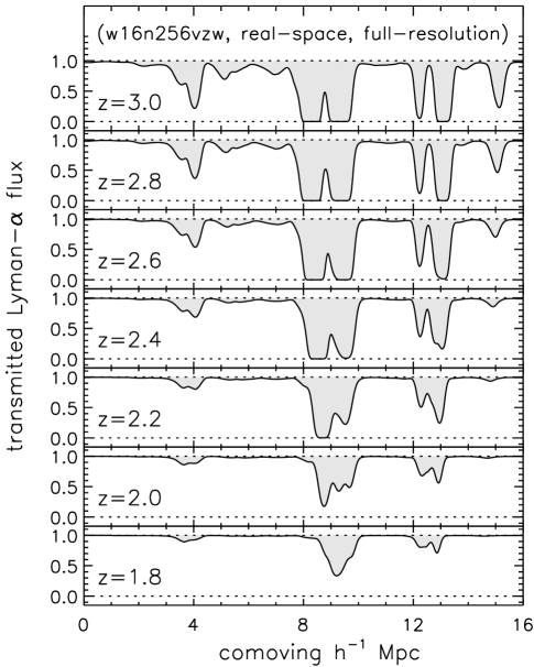
Figure 1.— Redshift evolution of the Ly$\alpha$ forest as seen in the same line of sight at $1.8<z<3$.

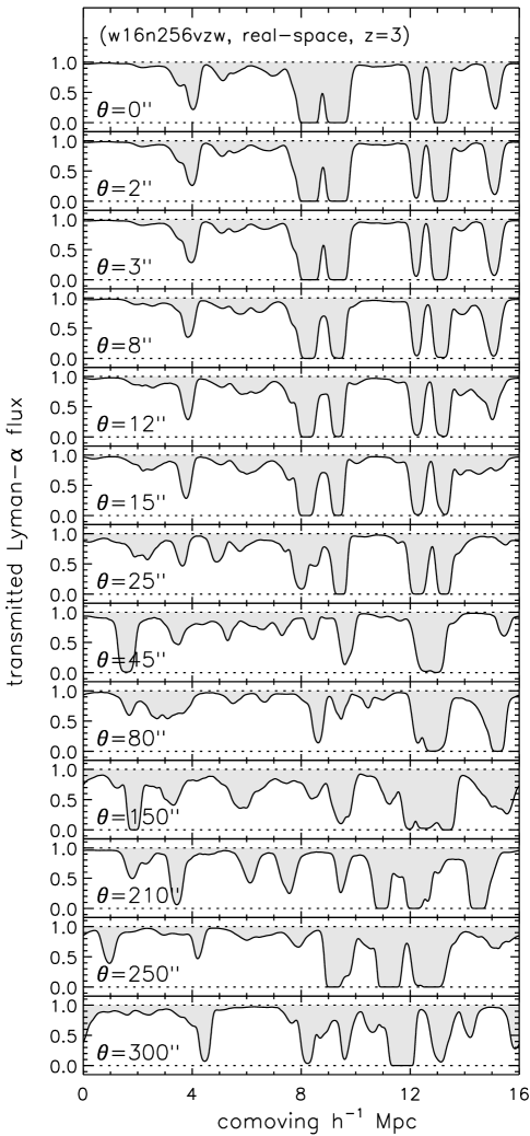
Figure 2.— One set of lines of sight illustrating how the cross-correlation diminishes with increasing separation.

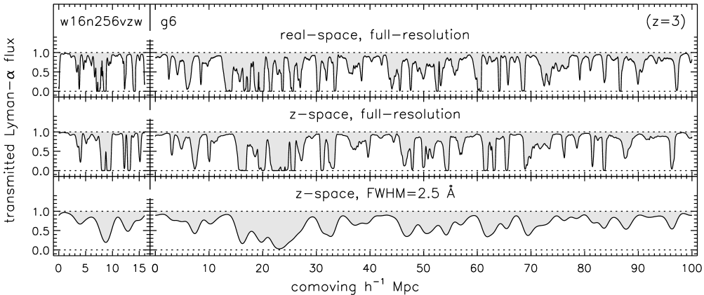
Figure 3.— Simulated spectra from wvzw and g6 show the larger box length (path length) of the latter, the higher mass resolution (narrower features) of the former, the subtle redistribution of opacity due to redshift-space distortions, and the smoothing effect of spectral resolution.

Figure 4.— In real-space, the correlation function is isotropic. However, in redshift-space, distortions caused by line-of-sight velocities affect the autocorrelation ($\xi_{\parallel}$) and cross-correlation ($\xi_{\perp}$) differently.

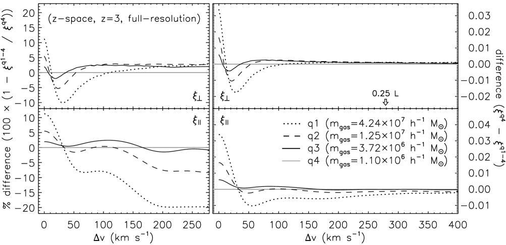
Figure 5.— Convergence of the cross-correlation (top) and autocorrelation (bottom) as a function of gas mass resolution for the q-series simulations ($L=10~{}h^{\textrm{-}1}$ comoving Mpc) which differ only by the number of particles.

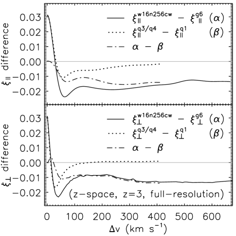
Figure 6.— Correlation difference between g6 and wcw (solid lines) primarily reflects the insufficient mass resolution of the former and box length of the latter. The signature of the mass resolution effect is illustrated by the dotted line, although for a smaller mass resolution difference. Accounting for the trend shown in Figure 5, the residual boxsize effect (dash-dotted lines) should be significantly flatter, particularly on the smallest scales ($\Delta v\,\scriptstyle\lesssim$ 50 km s${}^{\textrm{-}1}$).

Figure 7.— Spectral smoothing redistributes autocorrelation ($\xi_{\parallel}$) while suppressing cross-correlation ($\xi_{\perp}$) on all scales, introducing anisotropy to the correlation function.

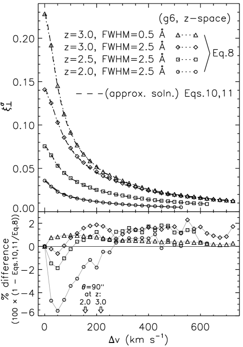
Figure 8.— Approximate solution for the suppression of cross-correlation due to spectral resolution, $\xi^{\sigma}_{\perp}\approx\xi_{\perp}\,\left(1+\left(\frac{1}{\xi^{\sigma}_{\parallel}\left(0\right)}-\frac{1}{\xi_{\perp}\left(0\right)}\right)\,\xi_{\perp}\right)^{\textrm{-}1}$, differs from the result based on smoothed spectra by $\scriptstyle\lesssim$ 2% for separations greater than 90 arcseconds.

Figure 9.— The $\Delta z=0.2$ sampling of wvzw shows that the redshift-evolution of the correlation function is monotonic and smooth, allowing reliable interpolation with a third order polynomial (solid and dotted lines).

Figure 10.— Mean flux decrement, $D_{\!A}$, of the Ly$\alpha$ forest remains observationally uncertain.

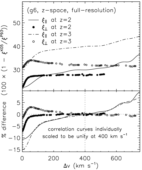
Figure 11.— Amplitude and shape of the Ly$\alpha$ flux correlation function are sensitive to the mean flux decrement, as evidenced by the relative difference in $\xi$ for simulated spectra tuned to match the values from Press et al. (1993, P93) and Kirkman et al. (2005, K05).

Figure 12.— Relative difference in autocorrelation corresponding to a 4% change in spectral resolution FWHM.

Figure 13.— Percent difference in correlation between wvzw and w16n256[cw/nw] indicates that Ly$\alpha$ correlation measurements are marginally affected by the prescription for galactic outflow. The preferred momentum-driven wind model vzw differs from the older constant wind model cw at $z=3$ and on scales larger than $\sim\,$50 km s${}^{\textrm{-}1}$ by $\scriptstyle\lesssim$ 1% for the cross-correlation and $\scriptstyle\lesssim$ 4% for the autocorrelation. This increases to $<\,5$% and $<\,7$%, respectively, when compared to no winds at all (nw).

Figure 14.— Ratios ($R$) in the left panels show the individual effects on the cross-correlation of spectral smoothing and redshift-space distortions at $z=3$ (top) and their combined impact at $z=2$, 2.5, and 3 (bottom). The relative difference between using the mean flux decrements measured by Press et al. (1993, P93) or Kirkman et al. (2005, K05) are given in the right panels.

Table 1Simulation Properties

Simulation		$L$		$N_{p}$	$m_{gas}$	$\epsilon\,$	Wind	Redshift		$N_{s}$
Name	Alias	($h^{-1}$ Mpc)			($h^{-1}$M☉)	($h^{-1}$ kpc)		Range	$\Delta z$
q1	$\cdots$	10		$2\times 64^{3}$	$4.24\times 10^{7}$	6.25	cw	3.0	$\cdots$	30000
q2	$\cdots$	10		$2\times 96^{3}$	$1.25\times 10^{7}$	4.17	cw	3.0	$\cdots$	30000
q3	$\cdots$	10		$2\times 144^{3}$	$3.72\times 10^{6}$	2.78	cw	3.0	$\cdots$	30000
q4	$\cdots$	10		$2\times 216^{3}$	$1.10\times 10^{6}$	1.85	cw	3.0	$\cdots$	30000
w16n256nw	wnw	16		$2\times 256^{3}$	$2.71\times 10^{6}$	1.25	nw	3.0	$\cdots$	20000
w16n256cw	wcw	16		$2\times 256^{3}$	$2.71\times 10^{6}$	1.25	cw	3.0	$\cdots$	20000
w16n256vzw	wvzw	16		$2\times 256^{3}$	$2.71\times 10^{6}$	1.25	vzw	$1.8-3.0$	0.2	20000
g6	$\cdots$	100		$2\times 484^{3}$	$9.79\times 10^{7}$	5.33	cw	$1.5-3.0$	0.5	3000

Note. — The columns (left to right) are: simulation name and abbreviation, box length, total number of particles, gas particle mass, equivalent Plummer gravitational softening length, wind model, redshift range and interval, and number of sets of lines of sight extracted along each of the three principal axes.

Table 2$D_{\!A}$ Variance

$z$	$\sigma^{2}_{D_{\!A}}\times l\,$
	wvzw	g6
1.5	$\cdots$	0.024144
1.8	0.041109	$\cdots$
2.0	0.048716	0.044152
2.2	0.056126	$\cdots$
2.4	0.063490	$\cdots$
2.5	$\cdots$	0.064115
2.6	0.069438	$\cdots$
2.8	0.074085	$\cdots$
3.0	0.076494	0.075647

Table 3Cross-Correlation (Press et al. (1993) Mean Flux Decrement)

$\Delta v$	$10\times\xi_{\perp}\!\left(\Delta v\right)$ in real-space								$10\times\xi_{\perp}\!\left(\Delta v\right)$ in z-space
($\delta v_{\perp}\!\left(z\right)$)	$z=1.8$	2.0	2.2	2.4	2.6	2.8	3.0		$z=1.8$	2.0	2.2	2.4	2.6	2.8	3.0
0000	0.4315	0.5914	0.7994	1.0641	1.4036	1.8199	2.3333		0.7489	0.9812	1.2594	1.5876	1.9748	2.4281	2.9558
0001	0.4263	0.5853	0.7917	1.0541	1.3907	1.8026	2.3094		0.7302	0.9614	1.2392	1.5660	1.9499	2.3995	2.9216
0002	0.4151	0.5702	0.7718	1.0275	1.3555	1.7566	2.2504		0.7089	0.9364	1.2103	1.5316	1.9089	2.3508	2.8630
0003	0.3997	0.5493	0.7436	0.9903	1.3067	1.6933	2.1686		0.6870	0.9090	1.1772	1.4915	1.8593	2.2893	2.7876
$\downarrow$
0300	0.0078	0.0107	0.0176	0.0230	0.0238	0.0237	0.0461		0.0489	0.0555	0.0654	0.0840	0.1030	0.1158	0.1270

Note. — These are the hybrid correlation values for full-resolution. [The complete version of this table can be found in the electronic edition of ApJ or upon request.]

Table 4Autocorrelation (Press et al. (1993) Mean Flux Decrement)

$\Delta v$	$10\times\xi_{\parallel}\!\left(\Delta v\right)$ in real-space								$10\times\xi_{\parallel}\!\left(\Delta v\right)$ in z-space
($\delta v_{\parallel}\!\left(z\right)$)	$z=1.8$	2.0	2.2	2.4	2.6	2.8	3.0		$z=1.8$	2.0	2.2	2.4	2.6	2.8	3.0
0000	0.4315	0.5914	0.7994	1.0641	1.4036	1.8199	2.3333		0.7489	0.9812	1.2594	1.5876	1.9748	2.4281	2.9558
0001	0.4250	0.5837	0.7902	1.0530	1.3902	1.8036	2.3135		0.7478	0.9797	1.2572	1.5847	1.9709	2.4231	2.9493
0002	0.4097	0.5649	0.7672	1.0249	1.3558	1.7616	2.2622		0.7445	0.9750	1.2507	1.5759	1.9593	2.4081	2.9303
0003	0.3897	0.5398	0.7359	0.9862	1.3079	1.7027	2.1899		0.7392	0.9674	1.2400	1.5615	1.9404	2.3838	2.8994
$\downarrow$
0999	7.5E-4	6.6E-5	-0.0019	-0.0023	0.0014	-0.0098	0.0026		-0.0028	-0.0042	-0.0060	-0.0078	-0.0094	-0.0116	-0.0114

Note. — These are the hybrid correlation values for full-resolution. [The complete version of this table can be found in the electronic edition of ApJ or upon request.]

Table 5Cross-Correlation (Kirkman et al. (2005) Mean Flux Decrement)

$\Delta v$	$10\times\xi_{\perp}\!\left(\Delta v\right)$ in real-space								$10\times\xi_{\perp}\!\left(\Delta v\right)$ in z-space
($\delta v_{\perp}\!\left(z\right)$)	$z=1.8$	2.0	2.2	2.4	2.6	2.8	3.0		$z=1.8$	2.0	2.2	2.4	2.6	2.8	3.0
0000	0.3219	0.4503	0.5798	0.7403	0.9426	1.1868	1.4890		0.5778	0.7721	0.9534	1.1649	1.4131	1.7022	2.0396
0001	0.3173	0.4449	0.5735	0.7323	0.9326	1.1738	1.4715		0.5596	0.7527	0.9342	1.1448	1.3905	1.6772	2.0107
0002	0.3078	0.4319	0.5569	0.7110	0.9052	1.1389	1.4279		0.5400	0.7295	0.9081	1.1144	1.3555	1.6371	1.9642
0003	0.2950	0.4143	0.5340	0.6817	0.8678	1.0918	1.3684		0.5204	0.7049	0.8793	1.0807	1.3151	1.5886	1.9065
$\downarrow$
0300	0.0057	0.0074	0.0119	0.0148	0.0139	0.0119	0.0274		0.0380	0.0400	0.0443	0.0570	0.0707	0.0786	0.0870

Note. — These are the hybrid correlation values for full-resolution. [The complete version of this table can be found in the electronic edition of ApJ or upon request.]

Table 6Autocorrelation (Kirkman et al. (2005) Mean Flux Decrement)

$\Delta v$	$10\times\xi_{\parallel}\!\left(\Delta v\right)$ in real-space								$10\times\xi_{\parallel}\!\left(\Delta v\right)$ in z-space
($\delta v_{\parallel}\!\left(z\right)$)	$z=1.8$	2.0	2.2	2.4	2.6	2.8	3.0		$z=1.8$	2.0	2.2	2.4	2.6	2.8	3.0
0000	0.3219	0.4503	0.5798	0.7403	0.9426	1.1868	1.4890		0.5778	0.7721	0.9534	1.1649	1.4131	1.7022	2.0396
0001	0.3162	0.4435	0.5721	0.7312	0.9320	1.1743	1.4742		0.5770	0.7709	0.9518	1.1628	1.4103	1.6987	2.0352
0002	0.3033	0.4275	0.5531	0.7087	0.9052	1.1425	1.4362		0.5746	0.7674	0.9471	1.1565	1.4022	1.6883	2.0221
0003	0.2868	0.4065	0.5277	0.6782	0.8685	1.0985	1.3834		0.5707	0.7616	0.9393	1.1463	1.3890	1.6715	2.0007
$\downarrow$
0999	6.4E-4	3.2E-5	-0.0011	-0.0015	0.0011	-0.0047	0.0012		-0.0021	-0.0030	-0.0041	-0.0054	-0.0067	-0.0083	-0.0084

Note. — These are the hybrid correlation values for full-resolution. [The complete version of this table can be found in the electronic edition of ApJ or upon request.]

Appendix A Autocorrelation Calculation for Arbitrary Spectral Resolution

One way to compute the simulated correlation function corresponding to a given spectral resolution is to carry out the calculations using spectra which have been individually smoothed as appropriate. However, assuming a Gaussian line spread function (LSF), the autocorrelation curve for data of arbitrary spectral resolution can also be obtained by simply convolving the full resolution curve with the LSF broadened by a factor of $\sqrt{2}$ (eqs. 4, 7, 8, and 10). The validity of this relation for our discrete, periodic simulated spectra has been tested and verified. Here, in the interest of clarity, we demonstrate its origin for the simplified case of continuous spectra. In this limit, equations 4, 7, and 8 become

$$\hat{\xi}_{\parallel}(\Delta v)=\frac{1}{N_{s}}\sum_{n=1}^{N_{s}}\frac{1}{N_{\perp}}\sum_{i=1}^{N_{\perp}}\frac{1}{\int dv_{\parallel}}\int\hat{\delta}_{n}\left(v_{\parallel},v_{\perp_{i}}\right)\,\hat{\delta}_{n}\left(v_{\parallel}+\Delta v,v_{\perp_{i}}\right)dv_{\parallel},$$ (A1)

$$\hat{\mathcal{S}}_{\parallel}\left[\hat{f}\left(v_{\parallel}\right),\sigma\right]=\int\hat{f}\left(\tau\right)\,\frac{1}{\sqrt{2\pi}\,\sigma}\,\,e^{\frac{-(v_{\parallel}-\tau)^{2}}{2\,\sigma^{2}}}d\tau,$$ (A2)

and

$$\hat{\xi}^{\sigma}_{\parallel}\left(\Delta v\right)=\frac{1}{N_{s}}\sum^{N_{s}}_{n=1}\frac{1}{N_{\perp}}\sum^{N_{\perp}}_{i=1}\frac{1}{\int dv_{\parallel}}\int\hat{\mathcal{S}}_{\parallel}\left[\hat{\delta}_{n}\left(v_{\parallel},v_{\perp_{i}}\right),\sigma\right]\,\hat{\mathcal{S}}_{\parallel}\left[\hat{\delta}_{n}\left(v_{\parallel}+\Delta v,v_{\perp_{i}}\right),\sigma\right]dv_{\parallel},$$ (A3)

respectively. Combining (A2) and (A3), and rearranging, yields

$$\hat{\xi}^{\sigma}_{\parallel}\left(\Delta v\right)=\frac{1}{N_{s}}\sum^{N_{s}}_{n=1}\frac{1}{N_{\perp}}\sum^{N_{\perp}}_{i=1}\frac{1}{\int dv_{\parallel}}\int\int\hat{\delta_{n}}\left(\tau,v_{\perp i}\right)\,\hat{\delta_{n}}\left(\tilde{\tau},v_{\perp i}\right)\,\int\frac{1}{2\pi\sigma^{2}}\,e^{\frac{-(v_{\parallel}-\tau)^{2}}{2\,\sigma^{2}}}e^{\frac{-(v_{\parallel}+\Delta v-\tilde{\tau})^{2}}{2\,\sigma^{2}}}dv_{\parallel}\,d\tau\,d\tilde{\tau}.$$ (A4)

After substituting $\beta\equiv v_{\parallel}-\tau$ and noting that $\int\frac{1}{2\pi\sigma^{2}}\,e^{\frac{-\beta^{2}}{2\sigma^{2}}}e^{\frac{-(\beta-\gamma)^{2}}{2\sigma^{2}}}d\beta=\frac{1}{2\sqrt{\pi}\sigma}e^{\frac{-\gamma^{2}}{4\sigma^{2}}}$, this becomes

$$\hat{\xi}^{\sigma}_{\parallel}\left(\Delta v\right)=\frac{1}{N_{s}}\sum^{N_{s}}_{n=1}\frac{1}{N_{\perp}}\sum^{N_{\perp}}_{i=1}\frac{1}{\int dv_{\parallel}}\int\int\hat{\delta_{n}}\left(\tau,v_{\perp i}\right)\,\hat{\delta_{n}}\left(\tilde{\tau},v_{\perp i}\right)\,\frac{1}{2\sqrt{\pi}\sigma}\,e^{\frac{-(\tilde{\tau}-\tau-\Delta v)^{2}}{4\sigma^{2}}}d\tau\,d\tilde{\tau}.$$ (A5)

With another change of variables ($\tilde{\tau}\equiv\tau+\alpha$), $\hat{\xi}^{\sigma}_{\parallel}$ can now be written in terms of (A1) and (A2):

$$\hat{\xi}^{\sigma}_{\parallel}\left(\Delta v\right) = \frac{1}{N_{s}}\sum^{N_{s}}_{n=1}\frac{1}{N_{\perp}}\sum^{N_{\perp}}_{i=1}\frac{1}{\int dv_{\parallel}}\int\int\hat{\delta_{n}}\left(\tau,v_{\perp i}\right)\,\hat{\delta_{n}}\left(\tau+\alpha,v_{\perp i}\right)\,\frac{1}{2\sqrt{\pi}\sigma}\,e^{\frac{-(\alpha-\Delta v)^{2}}{4\sigma^{2}}}d\tau\,d\alpha$$ (A6)

$$\hat{\xi}^{\sigma}_{\parallel}\left(\Delta v\right) = \int\left(\frac{1}{N_{s}}\sum^{N_{s}}_{n=1}\frac{1}{N_{\perp}}\sum^{N_{\perp}}_{i=1}\frac{1}{\int dv_{\parallel}}\int\hat{\delta_{n}}\left(\tau,v_{\perp i}\right)\,\hat{\delta_{n}}\left(\tau+\alpha,v_{\perp i}\right)\,d\tau\right)\frac{1}{\sqrt{2\pi}(\sqrt{2}\sigma)}\,e^{\frac{-(\alpha-\Delta v)^{2}}{2(\sqrt{2}\sigma)^{2}}}d\alpha$$ (A7)

$$\hat{\xi}^{\sigma}_{\parallel}\left(\Delta v\right) = \hat{\mathcal{S}}_{\parallel}\left[\hat{\xi}_{\parallel}\left(\Delta v\right),\sqrt{2}\sigma\right].$$ (A8)

References

- Aguirre et al. (2001) Aguirre, A., Hernquist, L., Schaye, J., Katz, N., Weinberg, D. H., & Gardner, J. 2001, ApJ, 561, 521
- Alcock & Paczynski (1979) Alcock, C., & Paczynski, B. 1979, Nature, 281, 358
- Bernardi et al. (2003) Bernardi, M., et al. 2003, AJ, 125, 32
- Cen et al. (1994) Cen, R., Miralda-Escudé, J., Ostriker, J. P., & Rauch, M. 1994, ApJ, 437, L9
- Coppolani et al. (2006) Coppolani, F., et al. 2006, MNRAS, 370, 1804
- Croft et al. (2002a) Croft, R. A. C., Hernquist, L., Springel, V., Westover, M., & White, M. 2002a, ApJ, 580, 634
- Croft et al. (2002b) Croft, R. A. C., Weinberg, D. H., Bolte, M., Burles, S., Hernquist, L., Katz, N., Kirkman, D., & Tytler, D. 2002b, ApJ, 581, 20
- Croft et al. (1998) Croft, R. A. C., Weinberg, D. H., Katz, N., & Hernquist, L. 1998, ApJ, 495, 44
- Croom et al. (2004) Croom, S. M., Smith, R. J., Boyle, B. J., Shanks, T., Miller, L., Outram, P. J., & Loaring, N. S. 2004, MNRAS, 349, 1397
- Davé et al. (1999) Davé, R., Hernquist, L., Katz, N., & Weinberg, D. H. 1999, ApJ, 511, 521
- Desjacques et al. (2004) Desjacques, V., Nusser, A., Haehnelt, M. G., & Stoehr, F. 2004, MNRAS, 350, 879
- Ferland et al. (1998) Ferland, G. J., Korista, K. T., Verner, D. A., Ferguson, J. W., Kingdon, J. B., & Verner, E. M. 1998, PASP, 110, 761
- Finlator et al. (2006) Finlator, K., Davé, R., Papovich, C., & Hernquist, L. 2006, ApJ, 639, 672
- Frye et al. (2003) Frye, B. L., Tripp, T. M., Bowen, D. B., Jenkins, E. B., & Sembach, K. R. 2003, in ASSL Vol. 281: The IGM/Galaxy Connection. The Distribution of Baryons at z=0, ed. J. L. Rosenberg & M. E. Putman, 231
- Haardt & Madau (1996) Haardt, F., & Madau, P. 1996, ApJ, 461, 20
- Haardt & Madau (2001) Haardt, F., & Madau, P. 2001, in Clusters of Galaxies and the High Redshift Universe Observed in X-rays, ed. D. M. Neumann & J. T. V. Tran
- Heckman et al. (2000) Heckman, T. M., Lehnert, M. D., Strickland, D. K., & Armus, L. 2000, ApJS, 129, 493
- Hernquist et al. (1996) Hernquist, L., Katz, N., Weinberg, D. H., & Miralda-Escudé, J. 1996, ApJ, 457, L51
- Hui et al. (1999) Hui, L., Stebbins, A., & Burles, S. 1999, ApJ, 511, L5
- Kaiser (1987) Kaiser, N. 1987, MNRAS, 227, 1
- Kim et al. (2001) Kim, T.-S., Cristiani, S., & D’Odorico, S. 2001, A&A, 373, 757
- Kirkman et al. (2005) Kirkman, D., et al. 2005, MNRAS, 360, 1373
- Lynds (1971) Lynds, R. 1971, ApJ, 164, L73
- Marble et al. (2008) Marble, A. R., Eriksen, K. A., Impey, C. D., Oppenheimer, B. D., & Davé, D. 2008, ApJS, 175, 29 (Paper I)
- Martin (1999) Martin, C. L. 1999, ApJ, 513, 156
- McDonald (2003) McDonald, P. 2003, ApJ, 585, 34
- McDonald & Miralda-Escudé (1999) McDonald, P., & Miralda-Escudé, J. 1999, ApJ, 518, 24
- McDonald et al. (2000) McDonald, P., Miralda-Escudé, J., Rauch, M., Sargent, W. L. W., Barlow, T. A., Cen, R., & Ostriker, J. P. 2000, ApJ, 543, 1
- McDonald et al. (2005) McDonald, P., Seljak, U., Cen, R., Bode, P., & Ostriker, J. P. 2005, MNRAS, 360, 1471
- McDonald et al. (2006) McDonald, P., et al. 2006, ApJS, 163, 80
- Meiksin & White (2004) Meiksin, A., & White, M. 2004, MNRAS, 350, 1107
- Oke & Korycansky (1982) Oke, J. B., & Korycansky, D. G. 1982, ApJ, 255, 11
- Oppenheimer & Davé (2006) Oppenheimer, B. D., & Davé, R. 2006, MNRAS, 373, 1265
- Petitjean et al. (1995) Petitjean, P., Mueket, J. P., & Kates, R. E. 1995, A&A, 295, L9
- Press et al. (1993) Press, W. H., Rybicki, G. B., & Schneider, D. P. 1993, ApJ, 414, 64
- Rauch (1998) Rauch, M. 1998, ARA&A, 36, 267
- Rollinde et al. (2003) Rollinde, E., Petitjean, P., Pichon, C., Colombi, S., Aracil, B., D’Odorico, V., & Haehnelt, M. G. 2003, MNRAS, 341, 1279
- Rupke et al. (2005) Rupke, D. S., Veilleux, S., & Sanders, D. B. 2005, ApJS, 160, 115
- Schaye et al. (2003) Schaye, J., Aguirre, A., Kim, T.-S., Theuns, T., Rauch, M., & Sargent, W. L. W. 2003, ApJ, 596, 768
- Seljak et al. (2003) Seljak, U., McDonald, P., & Makarov, A. 2003, MNRAS, 342, L79
- Spergel et al. (2007) Spergel, D. N., et al. 2007, ApJS, 170, 377
- Springel (2005) Springel, V. 2005, MNRAS, 364, 1105
- Springel & Hernquist (2003) Springel, V., & Hernquist, L. 2003, MNRAS, 339, 312
- Springel et al. (2001) Springel, V., Yoshida, N., & White, S. D. M. 2001, New Astronomy, 6, 79
- Theuns et al. (1998) Theuns, T., Leonard, A., Efstathiou, G., Pearce, F. R., & Thomas, P. A. 1998, MNRAS, 301, 478
- Weymann et al. (1981) Weymann, R. J., Carswell, R. F., & Smith, M. G. 1981, ARA&A, 19, 41
- Zaldarriaga et al. (2003) Zaldarriaga, M., Scoccimarro, R., & Hui, L. 2003, ApJ, 590, 1
- Zhang et al. (1995) Zhang, Y., Anninos, P., & Norman, M. L. 1995, ApJ, 453, L57