Cross sections of $e^{+}e^{-}\to\gamma VV$ and $e^{+}e^{-}\to\gamma\gamma V$

Abstract

Cross sections of the $e^{+}e^{-}$ annihilation into one photon plus two vector mesons, such as $J/\psi\rho$, $J/\psi\phi$, and $\rho\phi$ at the center of mass energy $\sqrt{s}=10.58~{}\mathrm{GeV}$ are calculated. These shed light on the measurement of the $e^{+}e^{-}$ annihilation cross section via radiative return in $B$-factories. At another center of mass energy $\sqrt{s}=3.097~{}\mathrm{GeV}$, namely the $J/\psi$ resonance peak, the processes $e^{+}e^{-}\to\gamma VV$ and $e^{+}e^{-}\to\gamma\gamma V$ (with $V$ being $\rho$, $\omega$, or $\phi$) are calculated with similar method. These calculations give estimation of the background levels in the study of radiative or double radiative decays of $J/\psi$.

I Introduction

The measurement of the $e^{+}e^{-}$ annihilation cross section via initial state radiation ($ISR$) turns out to be very fruitful at the $B$-factories due to the large data samples collected on the $\Upsilon(4S)$ resonance. The study of the final states with a charmonium ($J/\psi$ or $\psi(2S)$) and light hadrons such as $\pi^{+}\pi^{-}$ and $K^{+}K^{-}$ results in the discovery of many unexpected charmonium-like states, such as the $Y(4008)$, $Y(4260)$, $Y(4360)$, and $Y(4660)$ Aubert:2005rm ; Aubert:2006ge ; Yuan:2007sj ; Wang:2007ea . But one should notice that, $e^{+}e^{-}\to\gamma\rho J/\psi$ is actually an important background in the measurement of the $\pi^{+}\pi^{-}J/\psi$ production via $ISR$ processes Aubert:2005rm ; Yuan:2007sj ; and this is also true in the case when final state $\pi^{+}\pi^{-}\psi(2S)$ was concerned Aubert:2006ge ; Wang:2007ea . Another similar case is in the study of $K^{+}K^{-}J/\psi$ via $ISR$, here background from $\gamma\phi J/\psi$ should be considered. Actually, of a recent observation at Belle Yuan:2007bt , this background has been estimated and subtracted by a requirement on the $K^{+}K^{-}$ invariant mass does not agree with a $\phi$. While the subtraction of $\gamma\phi J/\psi$ background is possible due to the narrow width of the $\phi$ meson, it is almost impossible for the $\pi^{+}\pi^{-}J/\psi$ and $\pi^{+}\pi^{-}\psi(2S)$ case, where the $\pi^{+}\pi^{-}$ invariant mass distribution is not very different from the wide $\rho$ resonance, so a calculation of the cross section is desired.

At lower energies, in the studies of $J/\psi\to\gamma VV$ at BES Xu:2007ca ; Ablikim:2006dw ; Ablikim:2006ca , where $V$ denotes light neutral vector meson such as $\rho$ (or $\omega$, $\phi$), direct productions $e^{+}e^{-}\to\gamma VV$ are backgrounds too. Analogously, $e^{+}e^{-}\to\gamma\gamma V$ are backgrounds in the $J/\psi$ double radiative decay channels Xu:2004qj as well as in the energy region of few tens of $\mathrm{MeV}$ around $\phi$ resonance where processes $e^{+}e^{-}\to\omega\pi^{0}$ and $e^{+}e^{-}\to\rho\pi^{0}$ are measured at KLOE Ambrosino:2006hb ; Ambrosino:2007wf . We can see that, although the direct production of $e^{+}e^{-}\to\gamma VV$ or $e^{+}e^{-}\to\gamma\gamma V$ is believed only at order $\mathcal{O}(\alpha^{3})$, the high luminosity at the $\phi$, $B$-factories and the forthcoming BESIII will provide opportunities to explore these rare processes.

The process $e^{+}e^{-}\to$ hadrons at center of mass (CM) energy $\sqrt{s}$ far below the $\mathrm{Z}^{0}$ mass is dominated by annihilation via a single virtual photon with charge-conjugation parity $C=-1$. Recently BaBar Aubert:2006we presented the first observation of the exclusive reactions $e^{+}e^{-}\to\rho^{0}\rho^{0}$ and $e^{+}e^{-}\to\phi\rho^{0}$, in which the final states are even under charge conjugate, and therefore cannot be produced via just a single photon. A possible interpretation is that these $C=+1$ final states are produced in the two-virtual-photon annihilation processes, i.e., they arise from $e^{+}e^{-}$ annihilation into two virtual photons with each virtual photon converts into a vector meson. The rates predicted by the above mechanism can be computed unambiguously using the effective vector meson-photon couplings determined from the leptonic widths of the mesons. Based on this assumption, the authors of Ref. Davier:2006fu calculated the cross sections of series of these processes and the results are in good agreement with BaBar’s measurements.

In this article, we calculate the cross sections of several $e^{+}e^{-}\to\gamma VV$ processes, such as $e^{+}e^{-}$ annihilate into one photon plus $J/\psi\rho$, $J/\psi\phi$ and $\rho\phi$ at the CM energy $\sqrt{s}=10.58~{}\mathrm{GeV}$ using the same method proposed in Ref. Davier:2006fu . We also calculate $e^{+}e^{-}$ annihilate into one photon plus $VV$, where $VV$ denotes $\omega\phi$ or $\rho\phi$ at $\sqrt{s}=3.097~{}\mathrm{GeV}$, in addition to calculate $e^{+}e^{-}$ annihilate into two photons plus a $\rho$, a $\phi$ or an $\omega$. The structure of this paper is, after a short introduction of the model, we give some details of how to calculate the amplitude of $e^{+}e^{-}\to(n)\gamma(m)\gamma^{*}$, then the numerical results and finally a brief discussion.

II Amplitude of $e^{+}e^{-}\to(n)\gamma(m)\gamma^{*}$

Our motivation focuses on investigating the non-resonance contributions to the processes of $e^{+}e^{-}\to\gamma V_{1}V_{2}$ and $\gamma\gamma V$, where the vector mesons of $V_{1}$ and $V_{2}$ have different quark contents. We assume the generic reaction $e^{+}e^{-}\to\gamma V_{1}V_{2}$ proceeds via an intermediate $e^{+}e^{-}\to\gamma\gamma^{*}\gamma^{*}$ process, and the two virtual photons converting into $V_{1}$ and $V_{2}$ with effective couplings $e/f_{1}$ and $e/f_{2}$ respectively. Then the differential cross section simply reads as

$$\mathrm{d}\sigma_{\gamma V_{1}V_{2}}=\left(\frac{e}{f_{1}}\right)^{2}\left(\frac{e}{f_{2}}\right)^{2}\mathrm{d}\sigma_{\gamma\gamma^{*}_{1}\gamma^{*}_{2}}(m^{2}_{V_{1}},m^{2}_{V_{2}})\;,$$ (1)

where $\mathrm{d}\sigma_{\gamma\gamma^{*}_{1}\gamma^{*}_{2}}(m^{2}_{V_{1}},m^{2}_{V_{2}})$ is the differential cross section of $e^{+}e^{-}\to\gamma\gamma^{*}\gamma^{*}$, which depends on the virtual photon masses, i.e. the masses of final vector mesons. The effective photon-meson couplings can be directly defined using the leptonic widths of the vectors

$$\Gamma^{V}_{ee}=\frac{\alpha}{3}\left(\frac{e}{f_{V}}\right)^{2}m_{V}\;,$$ (2)

when narrow widths approximation is used. Notice that the $\rho$ meson cannot be described as a narrow vector meson properly for its somewhat large width, a complete consideration should take an integral over its mass distribution. But from a practical point of view the narrow width approximation works well, and the $\rho$ meson mass distribution only contribute a correction less than $8\%$ Davier:2006fu . So we will adopt narrow widths approximation in following computation. For another similar reaction $e^{+}e^{-}\to\gamma\gamma V$, the cross section formula is similar to Eq. (1) except one virtual photon be replaced by a real one as long as the interference between the two real photons can be neglected.

In order to calculate the cross sections of $e^{+}e^{-}\to\gamma VV$ or $e^{+}e^{-}\to\gamma\gamma V$, from Eq. (1) it’s clear that an essential work is to calculate the cross section of a pure QED process, which can be represented by a more general form $e^{+}e^{-}\to(n)\gamma(m)\gamma^{*}$, i.e. an electron and a positron annihilate into $n$ real and $m$ virtual photons. Although the amplitudes of these processes can be derived from corresponding Feynman diagrams unambiguously, the length of the calculation formulae should increase very fast and become very tedious even when $n+m=3$, let alone the finial states containing more than three photons. As the best to our knowledge, present calculations remain on the electron positron annihilation into three real photons Berends:1980px or two photons up to the next to leading order Rodrigo:2001jr . In practice we utilize two specific packages, FeynArts Hahn:2000kx and FeynCalc Mertig:1990an , within the symbol calculation tool Mathematica to do the programme work to overcome the complexity problem we mentioned above and to avoid the potential mistakes which may arise from the lengthy formulae. As our interest lies in those particular processes whose final states involving virtual photons, we introduce a new model package which contains additional time-like massive photons obey the same dynamics of the standard QED photons and should be considered as an extension to the built-in QED model. The Feynman diagrams of a relatively simple process $e^{+}e^{-}$ annihilate into one real photon and two virtual photons are depicted in Fig. 1 at tree order as an example.

Figure 1: Feynman diagrams of $e^{+}e^{-}\to\gamma\gamma^{*}\gamma^{*}$ at tree order.

For a general process $e^{-}(p_{1})e^{+}(p_{2})\to\gamma(k_{1})\gamma(k_{2})\gamma(k_{3})$, the starting point is the scattering formula wenberg

$$\mathrm{d}\sigma(\alpha\to\beta)\equiv\mathrm{d}\Gamma(\alpha\to\beta)/\Phi_{\alpha}=(2\pi)^{4}u^{-1}_{\alpha}|M_{\beta\alpha}|^{2}\delta^{4}(p_{\beta}-p_{\alpha})\mathrm{d}\beta$$ (3)

with

$$u_{\alpha}\equiv\frac{|\mathchoice{\mbox{\boldmath$\displaystyle p$}}{\mbox{\boldmath$\textstyle p$}}{\mbox{\boldmath$\scriptstyle p$}}{\mbox{\boldmath$\scriptscriptstyle p$}}|(E_{1}+E_{2})}{E_{1}E_{2}}\;.$$ (4)

Here we get $u=2$ when the electron and positron masses are neglected. $d\beta$ is the 3-body phase space. The corresponding amplitude

$$F\cdot M_{\beta\alpha}=\bar{v}(p_{2})\not{\epsilon}^{*}(k_{1})\frac{\not{k}_{1}-\not{p}_{2}}{(k_{1}-p_{2})^{2}}\not{\epsilon}^{*}(k_{2})\frac{\not{k}_{1}+\not{k}_{2}-\not{p}_{2}}{(k_{1}+k_{2}-p_{2})^{2}}\not{\epsilon}^{*}(k_{3})u(p_{1})+\{\mathrm{perm}(k_{1},k_{2},k_{3})\}$$ (5)

can be read from FeynArts directly with our modified-QED model, where $u,v$ are spinors of initial states, $\epsilon$’s are polarization vectors of final states, $p_{i}$ and $k_{i}$ are corresponding momenta, $\mathrm{perm}(k_{1},k_{2},k_{3})$ means all the possible permutation of $k_{1}$, $k_{2}$, and $k_{3}$. And $F=(2\pi)^{9/2}\sqrt{8E^{\prime}_{1}E^{\prime}_{2}E^{\prime}_{3}}$ is a scalar factor arising from the representation differences between FeynArts and FeynCalc packages. Here we use the standard Lorentz covariant formula derived from FeynArts instead of adopting the helicity form which is proposed in Ref. Kolodziej:1991pk just for the technical reason, because in Ref. Kolodziej:1991pk polarization vectors, fermion spinors, and amplitude matrices are all expressed in explicit forms. In order to speed up the numerical integral, we derive a new phase space formula in Lorentz covariant form:

$$\delta^{4}(p_{\beta}-p_{\alpha})\mathrm{d}\beta=\frac{|\mathchoice{\mbox{\boldmath$\displaystyle k$}}{\mbox{\boldmath$\textstyle k$}}{\mbox{\boldmath$\scriptstyle k$}}{\mbox{\boldmath$\scriptscriptstyle k$}}_{1}|^{2}|\mathchoice{\mbox{\boldmath$\displaystyle k$}}{\mbox{\boldmath$\textstyle k$}}{\mbox{\boldmath$\scriptstyle k$}}{\mbox{\boldmath$\scriptscriptstyle k$}}_{3}|\sin\theta_{1}\mathrm{d}\theta_{1}\mathrm{d}\theta_{3}\mathrm{d}\phi_{1}\mathrm{d}E^{\prime}_{1}\mathrm{d}E^{\prime}_{3}}{\sin\theta_{2}\sin(\phi_{2}-\phi_{3})}=\frac{|\mathchoice{\mbox{\boldmath$\displaystyle k$}}{\mbox{\boldmath$\textstyle k$}}{\mbox{\boldmath$\scriptstyle k$}}{\mbox{\boldmath$\scriptscriptstyle k$}}_{1}|^{2}|\mathchoice{\mbox{\boldmath$\displaystyle k$}}{\mbox{\boldmath$\textstyle k$}}{\mbox{\boldmath$\scriptstyle k$}}{\mbox{\boldmath$\scriptscriptstyle k$}}_{3}|\mathrm{d}\Omega_{1}\mathrm{d}\theta_{3}\mathrm{d}E^{\prime}_{1}\mathrm{d}E^{\prime}_{3}}{\sin\theta_{2}\sin(\phi_{2}-\phi_{3})}\;,$$ (6)

where the sum over all possible solutions of energy-momentum conservation respect to $\phi_{2}$ and $\phi_{3}$ is implied. The formula is derived with the transformation of $\delta$ function:

$$\delta(f_{1}(\theta_{1},\theta_{2}))\delta(f_{2}(\theta_{1},\theta_{2}))=\sum\delta(\theta_{1}-\theta^{0}_{1})\delta(\theta_{2}-\theta^{0}_{2})\left.A^{-1}\right|_{\theta_{1}=\theta^{0}_{1},\theta_{2}=\theta^{0}_{2}}\;,$$ (7)

where $f_{1}$ and $f_{2}$ are general functions depending on $\theta_{1}$ and $\theta_{2}$,

$$A=\mathrm{det}\left|{\frac{\partial f_{1}}{\partial\theta_{1}}\quad\frac{\partial f_{1}}{\partial\theta_{2}}\atop\frac{\partial f_{2}}{\partial\theta_{1}}\quad\frac{\partial f_{2}}{\partial\theta_{2}}}\right|\;,$$ (8)

and $\theta^{0}_{1}$ and $\theta^{0}_{2}$ are the solutions of equations $f_{1}(\theta_{1},\theta_{2})=0$ and $f_{2}(\theta_{1},\theta_{2})=0$, $\sum$ means a sum over all possible solutions. Considering the energy-momentum is conserved and the final state particles are on-shell, we obtain Eq. (6). Combining Eq. (3) with Eqs. (4), (5), and (6), we obtain the cross section formula used in our program footnote .

III Numerical results

With the amplitudes of $e^{+}e^{-}\to\gamma\gamma^{*}\gamma^{*}$ and $e^{+}e^{-}\to\gamma\gamma\gamma^{*}$, we obtain the cross sections of $e^{+}e^{-}\to\gamma VV$ and $e^{+}e^{-}\to\gamma\gamma V$ by Eq. (1). Since the final analytic results are extremely lengthy, we only provide the numerical results here for compactness. All the parameters used in our computation without explicit exception are quoted from PDG pdg:2006 . We show the cross sections of processes $e^{+}e^{-}\to\gamma VV$ at $\sqrt{s}=10.58~{}\mathrm{GeV}$ in Table 1, with $VV$ being $J/\psi\rho$, $J/\psi\phi$ and $\rho\phi$ when the invariant mass of the meson pair ranging from threshold to $5.2~{}\mathrm{GeV}/c^{2}$. As examples for illustration, the differential cross section of $e^{+}e^{-}\to\gamma J/\psi\rho$ versus the invariant mass of $J/\psi\rho$ is drawn in Fig. 2. Similarly, the cross sections of processes $e^{+}e^{-}\to\gamma VV$ at $\sqrt{s}=3.097~{}\mathrm{GeV}$ are exhibited in Table 2, this time $VV$ represents $\phi\omega$ or $\phi\rho$, with the invariant masses ranging from their thresholds to $3.0~{}\mathrm{GeV}/c^{2}$. Figure 3 shows the differential cross section of $e^{+}e^{-}\to\gamma\phi\rho$ versus the invariant mass of $\phi\rho$ as an example. Finally, we provide the cross sections of $e^{+}e^{-}\to\gamma\gamma V$ at $\sqrt{s}=3.097~{}\mathrm{GeV}$ in Table 3, here $V$ represents a single meson which is $\rho$, $\phi$ or $\omega$, with the invariant mass of one photon and one meson varying from their thresholds to $3.0~{}\mathrm{GeV}/c^{2}$. Here only the differential cross section of $e^{+}e^{-}\to\gamma\gamma\rho$ versus the invariant mass of a photon and $\rho$ is drawn in Fig. 4 as an example for the same compactness reason.

Table 1: The cross section of $e^{+}e^{-}\to\gamma VV$ at $\sqrt{s}=10.58~{}\mathrm{GeV}$.

final states		invariant mass of VV ($\mathrm{GeV}/c^{2}$)		$\sigma~{}(\mathrm{fb})$
$\gamma\ J/\psi\ \rho$		$3.8-5.2$		$0.29$
$\gamma\ J/\psi\ \phi$		$4.1-5.2$		$0.022$
$\gamma\ \rho\ \phi$		$1.7-5.2$		$0.66$

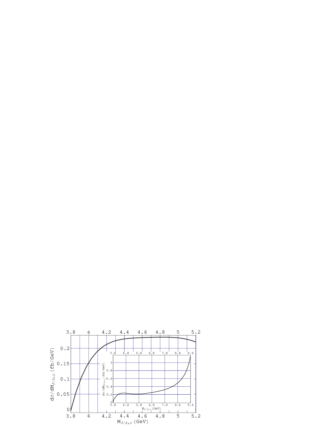
Figure 2: Differential cross section of $e^{+}e^{-}\to\gamma\gamma^{*}\gamma^{*}\to\gamma J/\psi\rho$ at $\sqrt{s}=10.58~{}\mathrm{GeV}$, the inset shows a wider mass range.

Table 2: The cross section of $e^{+}e^{-}\to\gamma VV$ at $\sqrt{s}=3.097~{}\mathrm{GeV}$.

final states		invariant mass of VV ($\mathrm{GeV}/c^{2}$)		$\sigma~{}(\mathrm{fb})$
$\gamma\ \phi\ \rho$		$1.7-3.0$		$9.68$
$\gamma\ \phi\ \omega$		$1.8-3.0$		$0.80$

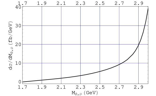
Figure 3: Differential cross section of $e^{+}e^{-}\to\gamma\gamma^{*}\gamma^{*}\to\gamma\phi\rho$ at $\sqrt{s}=3.097~{}\mathrm{GeV}$.

Table 3: The cross section of $e^{+}e^{-}\to\gamma\gamma V$ at $\sqrt{s}=3.097~{}\mathrm{GeV}$.

final states		invariant mass of VV ($\mathrm{GeV}/c^{2}$)		$\sigma~{}(\mathrm{pb})$
$\gamma\ \gamma\ \rho$		$0.7-3.0$		$49.30$
$\gamma\ \gamma\ \phi$		$1.0-3.0$		$6.75$
$\gamma\ \gamma\ \omega$		$0.8-3.0$		$3.96$

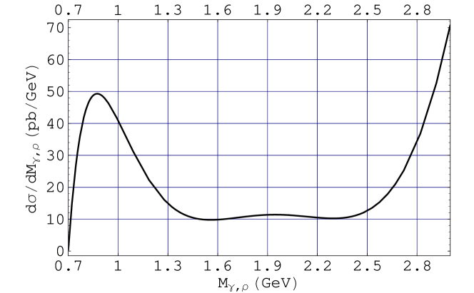
Figure 4: Differential cross section of $e^{+}e^{-}\to\gamma\gamma\gamma^{*}\to\gamma\gamma\rho$ at $\sqrt{s}=3.097~{}\mathrm{GeV}$.

IV Discussion

In this article, we calculate the cross sections of $e^{+}e^{-}$ annihilation into one photon plus $J/\psi\rho$, $J/\psi\phi$, or $\rho\phi$ at $\sqrt{s}=10.58~{}\mathrm{GeV}$; and one photon plus $\omega\phi$, $\rho\phi$, or $\gamma\rho$, $\gamma\phi$, or $\gamma\omega$ at $\sqrt{s}=3.097~{}\mathrm{GeV}$. The numerical results are shown in Tables 1, 2, and 3, and several differential cross sections are displayed as examples in Figs. 2, 3, and 4.

One essential component of our calculation is about the processes $e^{+}e^{-}\to(n)\gamma(m)\gamma^{*}$, here we only calculate $e^{+}e^{-}\to(1)\gamma(2)\gamma^{*}$ and $e^{+}e^{-}\to(2)\gamma(1)\gamma^{*}$ at leading order. However, it should be pointed out that our method is flexible and extensible, i.e., within the framework of our computation, the annihilation is a purely QED process, any number of photons and higher orders can be achieved without difficulty. For any extension, the whole method is standard, only a few collateral modifications need to be carried out within the computation frame. More details are given in the following paragraph. We should also mention that, up to now, we have neglected some possible corrections from such as hadronic contributions, higher order loops, weak interaction, product photons interference, and the mass distributions of the resonances. However, these corrections are small compared with the leading order contribution and far beyond the present experimental precision. Similarly, the above improvement can be achieved through just intuitive extensions of our present calculation.

Here we take some interesting deductions from our calculation such as $e^{+}e^{-}\to VV$ and $e^{+}e^{-}\to\gamma\gamma(\gamma)$. In addition to illustrate the flexibility of our method, these deductions also conform the validity of our computation by the consistencies between them and other literatures. First, it is obvious that when we reduce the number of photons from three to two, we are actually calculating $e^{+}e^{-}$ annihilation into two virtual photons. Then it is easy to get the cross sections with two-vector-meson final states such as $e^{+}e^{-}\to\omega J/\psi$, $e^{+}e^{-}\to\rho\phi$, and $e^{+}e^{-}\to\rho J/\psi$. It turns out that the results from our calculation are the same as those in Ref. Davier:2006fu . Note that the whole calculation is standard, only a few specific considerations are taken into during this reduction, such as the $2\to 2$ phase space and some ”package caused” factors fnote which are different from those in the process $2\to 3$. Second, we can fix all the final state virtual photons to be real, then actually we calculate the cross sections of $e^{+}e^{-}\to\gamma\gamma\gamma$. Similar to the above case, here we need only do a few peripheral modifications, that include fixing all the photon-masses to zero since the photons are on-shell now, setting the number of polarization directions to be two instead of previous three, and multiplying a factor $1/3!=1/6$ because now the final state contains just three identical bosons etc. Eventually our result of $e^{+}e^{-}$ annihilation into three real photons is consistent with both theoretical prediction Berends:1980px and experimental result Acciarri:1999cb . Finally, with a further reduction when we only calculate $e^{+}e^{-}$ annihilation into two real photons, the analytic formula returns to the familiar $(1+\cos^{2}\theta)/\sin^{2}\theta$ form. All the reductions we discussed above are easily realized in our program and their consistencies with other studies should be considered as verifications of our method.

Finally we want to mention two important features of our results. One is that if the phase space allowed, i.e. the CM energy is high enough for a specific final state, all the differential cross sections would show similar shapes. As what displayed in Figs. 2 and 4, with the invariant mass varying from low to high, there would be a bump near the threshold followed by a flat part and then ended with a fast increase when the invariant mass approaches the CM energy, which is resulted from a very soft radiated photon. The other feature is, as we expected, these three-photon processes are $\mathcal{O}(\alpha)$ suppressed compared with the corresponding $ISR$ processes where the hadron system is produced from a single photon. That means the backgrounds which arising directly from $e^{+}e^{-}\to\gamma VV$ and $e^{+}e^{-}\to\gamma\gamma V$ are not essential at $B$-factories in the study of the $ISR$ processes, nor at BES in $J/\psi$ decays at current available statistics. However, accompanying with the upcoming super-$B$ factory and BESIII, these modes will be important in the near future when more accumulated luminosity is achieved and a better precision is expected in various analyses.

References

• (1) B.ย Aubert et al. [BaBar Collaboration], Phys.ย Rev.ย Lett.ย  95, 142001 (2005) [arXiv:hep-ex/0506081].
• (2) B.ย Aubert et al. [BaBar Collaboration], Phys.ย Rev.ย Lett.ย  98, 212001 (2007) [arXiv:hep-ex/0610057].
• (3) C.ย Z.ย Yuan et al. [Belle Collaboration], Phys.ย Rev.ย Lett.ย  99, 182004 (2007) [arXiv:0707.2541 [hep-ex]].
• (4) X.ย L.ย Wang et al. [Belle Collaboration], Phys.ย Rev.ย Lett.ย  99, 142002 (2007) [arXiv:0707.3699 [hep-ex]].
• (5) C.ย Z.ย Yuan et al. [Belle Collaboration], Phys.ย Rev.ย  D 77, 011105 (2008) [arXiv:0709.2565 [hep-ex]].
• (6) M.ย Ablikim et al. [BES Collaboration], Phys.ย Rev.ย  D 77, 012001 (2008) [arXiv:0710.2979 [hep-ex]].
• (7) M.ย Ablikim et al. [BES Collaboration], Phys.ย Rev.ย Lett.ย  96, 162002 (2006) [arXiv:hep-ex/0602031].
• (8) M.ย Ablikim et al. [BES Collaboration], Phys.ย Rev.ย  D 73, 112007 (2006) [arXiv:hep-ex/0604045].
• (9) J.ย Z.ย Bai et al. [BES Collaboration], Phys.ย Lett.ย  B 594, 47 (2004) [arXiv:hep-ex/0403008].
• (10) F.ย Ambrosino et al. [KLOE Collaboration], Eur.ย Phys.ย J.ย  C 49, 473 (2007) [arXiv:hep-ex/0609009].
• (11) F.ย Ambrosino et al. [KLOE collaboration], arXiv:0707.4130 [hep-ex].
• (12) B.ย Aubert et al. [BaBar Collaboration], Phys.ย Rev.ย Lett.ย  97, 112002 (2006) [arXiv:hep-ex/0606054].
• (13) M.ย Davier, M.ย E.ย Peskin and A.ย Snyder, arXiv:hep-ph/0606155.
• (14) For the process $2e\to 2\gamma$, the scalar factor is $F=(2\pi)^{3}\sqrt{4E^{\prime}_{1}E^{\prime}_{2}}$.
• (15) F.ย A.ย Berends and R.ย Kleiss, Nucl.ย Phys.ย  B 186, 22 (1981).
• (16) G.ย Rodrigo, A.ย Gehrmann-De Ridder, M.ย Guilleaume and J.ย H.ย Kuhn, Eur.ย Phys.ย J.ย  C 22, 81 (2001) [arXiv:hep-ph/0106132].
• (17) T.ย Hahn, Comput.ย Phys.ย Commun.ย  140, 418 (2001) [arXiv:hep-ph/0012260].
• (18) R.ย Mertig, M.ย Bohm and A.ย Denner, Comput.ย Phys.ย Commun.ย  64, 345 (1991) [Web site of FeynCalc: http://www.feyncalc.org/].
• (19) Steven Wenberg, The quantum theory of fields, V1 P137, published by the Press Syndicate of th University of Cambridge (1995)
• (20) K.ย Kolodziej and M.ย Zralek, Phys.ย Rev.ย  D 43, 3619 (1991).
• (21) Actually we also need to average initial state and sum over all particular polarizations of the final state particles. In FeynCalc, for an arbitrary 4ร—4444\times 4 matrix A๐ดA, we use a built-in function FermionSpinSum[ย ] to construct the Traces out the squared amplitude โˆ‘ฯƒโ€‹ฯƒโ€ฒ|uยฏโ€‹(pโ€ฒ,ฯƒโ€ฒ)โ€‹Aโ€‹uโ€‹(p,ฯƒ)|2=Trโ€‹{Aโ€‹(โˆ’iโ€‹pฬธ+m2โ€‹p0)โ€‹ฮฒโ€‹Aโ€ โ€‹ฮฒโ€‹(โˆ’iโ€‹pฬธโ€ฒ+m2โ€‹pโ€ฒโฃ0)}subscript๐œŽsuperscript๐œŽโ€ฒsuperscriptยฏ๐‘ขsuperscript๐‘โ€ฒsuperscript๐œŽโ€ฒ๐ด๐‘ข๐‘๐œŽ2Tr๐ด๐‘–italic-pฬธ๐‘š2superscript๐‘0๐›ฝsuperscript๐ดโ€ ๐›ฝ๐‘–superscriptitalic-pฬธโ€ฒ๐‘š2superscript๐‘โ€ฒ0\sum_{\sigma\sigma^{\prime}}|\bar{u}(p^{\prime},\sigma^{\prime})Au(p,\sigma)|^{2}=\mathrm{Tr}\left\{A\left(\frac{-i\not{p}+m}{2p^{0}}\right)\beta A^{\dagger}\beta\left(\frac{-i\not{p}^{\prime}+m}{2p^{\prime 0}}\right)\right\}, and we use another built-in function PolarizationSum[ย ] to reduce the polarization sum: for real and virtual photons they are ฯตฮผโˆ—โ€‹(k)โ€‹ฯตฮฝโ€‹(k)=โˆ’gฮผโ€‹ฮฝsubscriptsuperscriptitalic-ฯต๐œ‡๐‘˜subscriptitalic-ฯต๐œˆ๐‘˜subscript๐‘”๐œ‡๐œˆ\epsilon^{*}_{\mu}(k)\epsilon_{\nu}(k)=-g_{\mu\nu} and ฯตฮผโˆ—โ€‹(k)โ€‹ฯตฮฝโ€‹(k)=kฮผโ€‹kฮฝ/k2โˆ’gฮผโ€‹ฮฝsubscriptsuperscriptitalic-ฯต๐œ‡๐‘˜subscriptitalic-ฯต๐œˆ๐‘˜subscript๐‘˜๐œ‡subscript๐‘˜๐œˆsuperscript๐‘˜2subscript๐‘”๐œ‡๐œˆ\epsilon^{*}_{\mu}(k)\epsilon_{\nu}(k)=k_{\mu}k_{\nu}/k^{2}-g_{\mu\nu} respectively.
• (22) W.-M.ย Yao et al. [Particle Data Group], J. Phys. G 33, 1 (2006).
• (23) M.ย Acciarri et al. [L3 Collaboration], Phys.ย Lett.ย  B 475, 198 (2000) [arXiv:hep-ex/0002036].