Method of Fundamental Solutions with
Optimal Regularization Techniques for
the Cauchy Problem of the Laplace Equation
with Singular Points

Abstract

The purpose of this study is to propose a high-accuracy and fast numerical method for the Cauchy problem of the Laplace equation. Our problem is directly discretized by the method of fundamental solutions (MFS). The Tikhonov regularization method stabilizes a numerical solution of the problem for given Cauchy data with high noises. The accuracy of the numerical solution depends on a regularization parameter of the Tikhonov regularization technique and some parameters of MFS. The L-curve determines a suitable regularization parameter for obtaining an accurate solution. Numerical experiments show that such a suitable regularization parameter coincides with the optimal one. Moreover, a better choice of the parameters of MFS is numerically observed. It is noteworthy that a problem whose solution has singular points can successfully be solved. It is concluded that the numerical method proposed in this paper is effective for a problem with an irregular domain, singular points, and the Cauchy data with high noises.

,

1 Introduction

Many kinds of inverse problems have recently been studied in science and engineering. The Cauchy problem of an elliptic partial differential equation is a well known inverse problem. The Cauchy problem of the Laplace equation is an important problem which can be applied to inverse problem of electrocardiography [12]. Onishi et al. [9] proposed an iterative method for solving the Cauchy problem of the Laplace equation. This method reduces the original inverse problem to an iterative process which alternatively solves two direct problems. This method, called the adjoint method in the papers [7], [10], can solve various inverse problems by applying many kinds of numerical methods for solving partial differential equations, such as the finite difference method (FDM), the finite element method (FEM), and the boundary element method (BEM). The convergence of this method for the Cauchy problem of the Laplace equation has been obtained [6].

The method of fundamental solutions (MFS) is effective for easily and rapidly solving the elliptic well-posed direct problems in complicated domains. Mathon and Johnston [13] first showed numerical results obtained by the MFS. The papers [11], [14] discuss some mathematical theories on the MFS. Both of the BEM and the MFS are well known boundary methods, which discretize original problems based on the fundamental solutions. The MFS does not require any treatments for the singularity of the fundamental solution, while the BEM requires singular integrals. The MFS is a true meshless method, and can easily be extended to higher dimensional cases.

Wei et al. [4] applied the MFS to the Cauchy problems of elliptic equations. This method uses the source points distributed outside the domain. The accuracy of numerical solutions depends on the location of the source points. They numerically showed the relation between the accuracy and the radius of a circle where the source points are distributed. But, the relation between the accuracy and the number of source points has not clearly been given, yet.

Many researchers have solved the Cauchy problem by various methods. However, to our knowledge, the conventional methods cannot solve a problem whose solution has singular points (see [8] for example).

In this paper, we use the MFS to directly discretize the Cauchy problem of the Laplace equation. This problem is an ill-posed problem, where the solution has no continuous dependence on the boundary data. Namely, a small noise contained in the given Cauchy data has a possibility to affect sensitively on the accuracy of the solution. The problem is discretized directly by the MFS and an ill-conditioned matrix equation is obtained. A numerical solution of the ill-conditioned equation is unstable. The singular value decomposition (SVD) can give an acceptable solution to such an ill-conditioned matrix equation. The SVD was successfully applied to the MFS for solving a direct problem [15]. Even though we apply the SVD, we still cannot obtain an acceptable solution for the case of the noisy Cauchy data. We use the Tikhonov regularization to obtain a stable regularized solution of the ill-conditioned equation. The regularized solution depends on a regularization parameter. Then, we need to determine a suitable regularization parameter to obtain a better regularized solution. Hansen [1] suggested the L-curve as a method for finding the suitable regularization parameter. It is known that the suitable parameter is the one corresponding to a regularized solution near the “corner” of the L-curve. We can find the corner of the L-curve as a point with the maximum curvature [5].

Under the assumption of uniform distribution of the source and the collocation points, we will numerically indicate that a suitable regularized solution obtained by the L-curve is optimal in the sense that the error is minimized. We will respectively show the accuracy and the optimal regularization parameter against a noise level. We will also mention influence of the total numbers of the source and the collocation points on accuracy. We will show that our method is effective for a problem whose solution has singular points. It is noteworthy that such kind of problems can also successfully be solved.

Section 2 introduces the Cauchy problem. In Section 3, the MFS discretizes the problem. In Section 4, the singular value decomposition, the Tikhonov regularization and the L-curve are used to obtain a suitable regularized solution. In Section 5, numerical experiments confirm that the suitable regularization parameter by the L-curve coincides with the optimal one that minimizes the error between the regularized solution and the exact one. The error and the optimal regularization parameter against the noise level of the Cauchy data are respectively shown. Then, our interest is how to choose the following three parameters used in MFS: the numbers of collocation points, the number of source points, and the radius of a circle where source points are distributed. A better choice of the parameters is also observed. A problem with an irregular domain and a problem whose solution has singular points are successfully solved, respectively. Section 6 concludes the paper.

2 Problem Setting

We consider the Laplace equation $-\Delta u=0$ in a two-dimensional bounded domain $\Omega$ enclosed by the boundary $\Gamma$. We prescribe Dirichlet and Neumann boundary conditions simultaneously on a part of the boundary $\Gamma$, denoted by $\Gamma_{1}$, as follows:

$$u=f,\quad\frac{\partial u}{\partial n}=g\quad\text{on}\quad\Gamma_{1},$$

where $f$ and $g$ denote given continuous functions defined on $\Gamma_{1}$, and $n$ the unit outward normal to $\Gamma_{1}$. Then, we need to find the boundary value $u$ on the rest of the boundary $\Gamma_{2}:=\Gamma\setminus\Gamma_{1}$ or the potential $u$ in the domain $\Omega$. This problem is called the Cauchy problem of the Laplace equation, and the boundary data are called the Cauchy data.

Our Cauchy problem is described as follows:

Problem 1

For the given Cauchy data $f,g\in C(\Gamma_{1})$, find $u\in C(\Gamma_{2})$ or $u\in C^{2}(\Omega)\cap C^{1}(\overline{\Omega})$ such that

$$-\Delta u =0 \Omega,$$ in (1)

$$u=f,\quad\frac{\partial u}{\partial n} =g \Gamma_{1}.$$ on (2)

The Cauchy problem is a well known ill-posed problem. We can show the instability of the solution to the Cauchy problem of the Laplace equation as follows: For example, in the case where

$$\Omega =(0,1)^{2}=\{(x,y):0<x<1,\ 0<y<1\},$$

$$\Gamma =[0,1]\times\{0\}=\{(x,0):0\leq x\leq 1\},$$

$$f(x,0) =\frac{1}{n^{k}}\sin(nx),\quad g(x,0)=0\quad(k>0),$$

the solution is given by

$$u(x,y)=\frac{1}{n^{k}}\sin(nx)\cosh(ny).$$

Here, we can see that

$$\sup_{{\boldsymbol{x}}\in\Gamma}|f({\boldsymbol{x}})|\to 0,\qquad\sup_{{\boldsymbol{x}}\in\overline{\Omega}}|u({\boldsymbol{x}})|\to\infty,$$

from which we know that the solution $u$ of the Cauchy problem does not depend continuously on the Cauchy data $f$ and $g$.

3 Discretization by the Method of Fundamental Solutions

Figure 1: Problem setting and distributions of collocation and source points

The fundamental solution of the Laplace equation in two dimensions is defined as

$$\varphi^{*}(r):=-\frac{1}{2\pi}\ln r$$

for $r=|{\boldsymbol{x}}|=\sqrt{x^{2}+y^{2}}$, which is a solution to

$$-\Delta\varphi^{*}=\delta({\boldsymbol{x}}).$$

We distribute the collocation points $\{{\boldsymbol{x}}_{i}\}_{i=1}^{M}\subset\Gamma_{1}$ on the boundary where the Cauchy data are prescribed, and the source points $\{{\boldsymbol{\xi}}_{j}\}_{j=1}^{N}\subset\overline{\Omega}^{c}$ along a circle outside the domain (Figure 1). We approximate $u$ by $u_{N}$:

$$u({\boldsymbol{x}})\approx u_{N}({\boldsymbol{x}}):=\sum_{j=1}^{N}w_{j}\varphi_{j}({\boldsymbol{x}}),$$ (3)

where the basis function is defined as

$$\varphi_{j}({\boldsymbol{x}}):=\varphi^{*}(|{\boldsymbol{x}}-{\boldsymbol{\xi}}_{j}|)$$ (4)

and $\{w_{j}\}_{j=1}^{N}$ are expansion coefficients to be determined below. Since the basis functions (4) have no singular points in $\Omega$, the approximate function $u_{N}$ satisfies the Laplace equation (1). Substituting (3) into (2) and assuming that (2) is satisfied at the collocation points, we have

$$\left\{\begin{split}\sum_{j=1}^{N}w_{j}\varphi_{j}({\boldsymbol{x}}_{i})&=f({\boldsymbol{x}}_{i}),\\ \sum_{j=1}^{N}w_{j}\frac{\partial\varphi_{j}}{\partial n}({\boldsymbol{x}}_{i})&=g({\boldsymbol{x}}_{i}),\end{split}\right.\quad i=1,2,\ldots,M$$

or in the matrix form:

$$A{\boldsymbol{w}}={\boldsymbol{b}},$$ (5)

where the matrix $A=(a_{ij})\in{\boldsymbol{R}}^{2M\times N}$ and the vectors ${\boldsymbol{w}}=(w_{j})\in{\boldsymbol{R}}^{N}$, ${\boldsymbol{b}}=(b_{i})\in{\boldsymbol{R}}^{2M}$ are defined by

$$a_{ij} :=\left\{\begin{array}[]{cl}\varphi_{j}({\boldsymbol{x}}_{i}),&i=1,2,\ldots,M\\ \displaystyle\frac{\partial\varphi_{j}}{\partial n}({\boldsymbol{x}}_{i-M}),&i=M+1,M+2,\ldots,2M\end{array}\right.,\quad j=1,2,\ldots,N,$$

$$b_{i} :=\left\{\begin{array}[]{cl}f({\boldsymbol{x}}_{i}),&i=1,2,\ldots,M\\ g({\boldsymbol{x}}_{i-M}),&i=M+1,M+2,\ldots,2M\end{array}\right..$$

4 Regularized Solution

4.1 Singular value decomposition

In general, (5) has the case where the exact solution ${\boldsymbol{w}}$ does not exist in the conventional sense. As an exact solution, we consider the least square and least norm solution ${\boldsymbol{w}}_{0}$ defined by

$$\|{\boldsymbol{w}}_{0}\|=\min_{{\boldsymbol{w}}\in W}\|{\boldsymbol{w}}\|,\quad W:=\{\widehat{{\boldsymbol{w}}}:\|A\widehat{{\boldsymbol{w}}}-{\boldsymbol{b}}\|=\min_{{\boldsymbol{w}}\in{\boldsymbol{R}}^{N}}\|A{\boldsymbol{w}}-{\boldsymbol{b}}\|\}.$$ (6)

In this paper, we refer the solution ${\boldsymbol{w}}_{0}$ as the exact solution to (5).

For the matrix $A\in{\boldsymbol{R}}^{2M\times N}$, the singular value decomposition (SVD) can be written as follows:

$$A=U\Sigma V^{T}=\sum_{i=1}^{r}\sigma_{i}{\boldsymbol{u}}_{i}{\boldsymbol{v}}_{i}^{T},$$

where

$$U=({\boldsymbol{u}}_{1}\ {\boldsymbol{u}}_{2}\ \cdots\ {\boldsymbol{u}}_{2M})\in{\boldsymbol{R}}^{2M\times 2M},\qquad V=({\boldsymbol{v}}_{1}\ {\boldsymbol{v}}_{2}\ \cdots\ {\boldsymbol{v}}_{N})\in{\boldsymbol{R}}^{N\times N},$$

$$\Sigma=(s_{ij})\in{\boldsymbol{R}}^{2M\times N},\qquad s_{ij}=\left\{\begin{array}[]{cc}\sigma_{i}&(i=j)\\ 0&(i\neq j)\end{array}\right.,$$

$$UU^{T}=I_{2M}\in{\boldsymbol{R}}^{2M\times 2M},\qquad VV^{T}=I_{N}\in{\boldsymbol{R}}^{N\times N},$$

$$2M\geq N,\qquad\sigma_{1}\geq\cdots\sigma_{r}>0,\quad\sigma_{r+1}=\cdots=\sigma_{N}=0$$

with the identity matrices $I_{2M}$ and $I_{N}$. The non-negative values $\{\sigma_{i}\}_{i=1}^{N}$ are called the singular values of the matrix $A$. Using the SVD, we can express the solution to (6) as

$${\boldsymbol{w}}_{0}=\sum_{i=1}^{r}\frac{({\boldsymbol{u}}_{i},{\boldsymbol{b}})}{\sigma_{i}}{\boldsymbol{v}}_{i}.$$

In a real problem, the Cauchy data $f$ and $g$ contain some noises. We consider the following equation instead of (5):

$$A{\boldsymbol{w}}={\boldsymbol{b}}^{\delta},\qquad{\boldsymbol{b}}^{\delta}={\boldsymbol{b}}+\Delta{\boldsymbol{b}}$$ (7)

with the noise vector $\Delta{\boldsymbol{b}}\in{\boldsymbol{R}}^{2M}$. Then, the solution ${\boldsymbol{w}}_{0}^{\delta}$ to

$$\|{\boldsymbol{w}}_{0}^{\delta}\|=\min_{{\boldsymbol{w}}\in W^{\delta}}\|{\boldsymbol{w}}\|,\quad W^{\delta}:=\{\widehat{{\boldsymbol{w}}}:\|A\widehat{{\boldsymbol{w}}}-{\boldsymbol{b}}^{\delta}\|=\min_{{\boldsymbol{w}}\in{\boldsymbol{R}}^{N}}\|A{\boldsymbol{w}}-{\boldsymbol{b}}^{\delta}\|\}$$ (8)

is quite different from the exact solution ${\boldsymbol{w}}_{0}$ to (6) since the solution is discontinuous for the Cauchy data. We need to find a good approximation to ${\boldsymbol{w}}_{0}$.

4.2 Tikhonov regularization

In order to obtain a good approximate solution to (8), we consider minimizing the following functional with a regularization parameter $\alpha>0$ according to the Tikhonov regularization:

$$J_{\alpha}^{\delta}({\boldsymbol{w}}):=\|A{\boldsymbol{w}}-{\boldsymbol{b}}^{\delta}\|^{2}+\alpha^{2}\|{\boldsymbol{w}}\|^{2}.$$ (9)

It is easy to see that the functional $J_{\alpha}^{\delta}$ is strictly convex for any $\alpha>0$. Hence, $J_{\alpha}^{\delta}$ has a unique minimum point ${\boldsymbol{w}}_{\alpha}^{\delta}$ called the regularized solution:

$$J_{\alpha}^{\delta}({\boldsymbol{w}}_{\alpha}^{\delta})=\min_{{\boldsymbol{w}}\in{\boldsymbol{R}}^{N}}J_{\alpha}^{\delta}({\boldsymbol{w}}).$$

We know that ${\boldsymbol{w}}_{\alpha}^{\delta}$ is the solution to

$$(A^{T}A+\alpha^{2}I_{N}){\boldsymbol{w}}_{\alpha}^{\delta}=A^{T}{\boldsymbol{b}}^{\delta}.$$ (10)

The equation (10) is uniquely solvable since the matrix $(A^{T}A+\alpha^{2}I_{N})$ is symmetric positive definite. The SVD of ${\boldsymbol{w}}_{\alpha}^{\delta}$ can be expressed in the form:

$${\boldsymbol{w}}_{\alpha}^{\delta}=\sum_{i=1}^{r}\gamma_{i}\frac{({\boldsymbol{u}}_{i},{\boldsymbol{b}}^{\delta})}{\sigma_{i}}{\boldsymbol{v}}_{i}$$

with the filter factor $\gamma_{i}:={\sigma_{i}^{2}}/({\sigma_{i}^{2}+\alpha^{2}})$. Then, substituting ${\boldsymbol{w}}_{\alpha}^{\delta}$ into (3), we find the approximate potential $u_{N}$ in $\Omega\cup\Gamma_{2}$.

The error between the regularized solution for the noisy data and the exact solution is decomposed into

$${\boldsymbol{w}}_{\alpha}^{\delta}-{\boldsymbol{w}}_{0}=({\boldsymbol{w}}_{\alpha}^{\delta}-{\boldsymbol{w}}_{\alpha}^{0})+({\boldsymbol{w}}_{\alpha}^{0}-{\boldsymbol{w}}_{0})=\sum_{i=1}^{r}\gamma_{i}\frac{({\boldsymbol{u}}_{i},\Delta{\boldsymbol{b}})}{\sigma_{i}}{\boldsymbol{v}}_{i}+\sum_{i=1}^{r}(\gamma_{i}-1)\frac{({\boldsymbol{u}}_{i},{\boldsymbol{b}})}{\sigma_{i}}{\boldsymbol{v}}_{i}.$$ (11)

The first term is the perturbation error due to the relative noise $\Delta{\boldsymbol{b}}$ and the second term is the regularization error caused by regularization of the exact ${\boldsymbol{b}}$. When $0<\alpha\ll 1$, we see that $\gamma_{i}\approx 1$ for most of $i$, and the error ${\boldsymbol{w}}_{\alpha}^{\delta}-{\boldsymbol{w}}_{0}$ is dominated by the perturbation error. On the other hand, when $\alpha\gg 1$, we see that $\gamma_{i}\ll 1$ and the error ${\boldsymbol{w}}_{\alpha}^{\delta}-{\boldsymbol{w}}_{0}$ is dominated by the regularization error. In the next subsection, we will consider a useful method for finding a suitable regularization parameter to minimize both of the perturbation and the regularization errors.

4.3 L-curve

To find a suitable regularization parameter, Hansen [1] suggests the L-curve, which is defined as the continuous curve consisting of all the point $(\|A{\boldsymbol{w}}_{\alpha}^{\delta}-{\boldsymbol{b}}^{\delta}\|,\|{\boldsymbol{w}}_{\alpha}^{\delta}\|)$ for $\alpha>0$:

$${\cal L}:=\{(\|A{\boldsymbol{w}}_{\alpha}^{\delta}-{\boldsymbol{b}}^{\delta}\|,\|{\boldsymbol{w}}_{\alpha}^{\delta}\|):\alpha>0\}.$$

For fixed $\alpha>0$, we get ${\boldsymbol{w}}_{\alpha}^{\delta}$ and then can calculate the residual norm $\|A{\boldsymbol{w}}_{\alpha}^{\delta}-{\boldsymbol{b}}^{\delta}\|$ and the solution norm $\|{\boldsymbol{w}}_{\alpha}^{\delta}\|$. Thus, the L-curve can be plotted as a set of all the points of the residual norms as abscissa and the solution norms as ordinate for all $\alpha>0$.

The L-curve is plotted in double logarithm, and displays the compromise between minimization of the perturbation error and the regularization error in (11). A suitable regularization parameter is given by the one corresponding to a regularized solution near the “corner” of the L-curve. The “corner” can be regarded as the point where the curvature of the L-curve becomes maximum [3], [5].

In the case when $2M=N$ and the Cauchy data $f,g$ have no noises, if $A$ is non-singular, we can directly solve (5) to obtain a solution with high accuracy. However, we cannot guarantee that (5) is always solvable. Even if there exists the inverse matrix, the solution to (5) for the noisy Cauchy data differs from the exact solution. On the other hand, the regularized solution by the Tikhonov regularization is always uniquely determined for $\alpha>0$. In the next section, our numerical experiments will show that the suitable regularization parameter given by L-curve coincides with the optimal one $\alpha_{\rm opt}$ defined by

$$\|{\boldsymbol{w}}_{0}-{\boldsymbol{w}}_{\alpha_{\rm opt}}^{\delta}\|=\min_{\alpha>0}\|{\boldsymbol{w}}_{0}-{\boldsymbol{w}}_{\alpha}^{\delta}\|.$$

5 Numerical Experiments

5.1 Circular domain

We first consider a harmonic function $u(x,y)=e^{x}\cos y-e^{y}\sin x$ in a unit disk $\Omega:=\{(x,y):x^{2}+y^{2}<1\}$. According to the exact potential $u$, the exact Cauchy data are given by $f=u$ and $g=\partial u/\partial n$ on the fourth part of the whole boundary $\Gamma$, which is defined by

$$\Gamma_{1}:=\{(x,y):x^{2}+y^{2}=1,\ x>0,\ y>0\}.$$

We now assume that the exact potential $u$ is unknown, and identify a boundary value on the rest of the boundary $\Gamma_{2}:=\partial\Omega\setminus\Gamma_{1}$ from the noisy Cauchy data $f^{\delta}=(1+\varepsilon)f$ and $g^{\delta}=(1+\varepsilon)g$, where $\varepsilon=\varepsilon(x,y)$ is a uniform random noise such that $-\delta\leq\varepsilon(x,y)\leq\delta$ with the relative noise level of $100\delta\%$.

We distribute uniformly the collocation points $\{{\boldsymbol{x}}_{i}\}_{i=1}^{M}\subset\Gamma_{1}$ and the source points $\{{\boldsymbol{\xi}}_{j}\}_{j=1}^{N}\subset\overline{\Omega}^{c}$ as follows:

$$\left\{\begin{split}{\boldsymbol{x}}_{i}&=(\cos\theta_{i},\sin\theta_{i}),\quad\theta_{i}=\frac{2\pi(i-1)}{4M}+\frac{\pi}{4M},\quad i=1,2,\ldots,M,\\ {\boldsymbol{\xi}}_{j}&=(R\cos\widehat{\theta}_{j},R\sin\widehat{\theta}_{j}),\quad\widehat{\theta}_{j}=\frac{2\pi(j-1)}{N}+\frac{\pi}{N},\quad j=1,2,\ldots,N,\end{split}\right.$$ (12)

where $R>1$ is the radius of the circle where the source points are distributed. We adopt the MATLAB code for solving discrete ill-posed problems based on SVD, made by Hansen [2], [3], to our numerical computations. Due to the maximum principle, it is sufficient to confirm the boundary error between the identified potential $u_{N}$ and the exact one $u$ rather than the domain error in our numerical experiments. We define the maximum relative error on the boundary by

$$e:=\frac{\|u_{N}-u\|_{\infty}}{\|u\|_{\infty}},$$

where the maximum norm on the boundary denotes

$$\|u\|_{\infty}=\sup_{{\boldsymbol{x}}\in\Gamma}|u({\boldsymbol{x}})|,\qquad\forall u\in C(\Gamma).$$

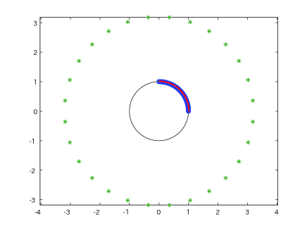
Figure 2: Distributions of collocation and source points ($(R,M,N)=(3.2,600,28)$)

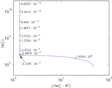
Figure 3: L-curve (The corner is located at the point for $\alpha=2.1195\times 10^{-3}$)

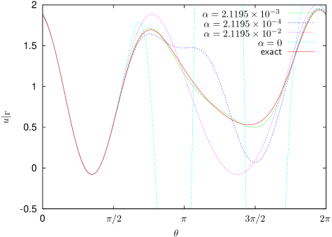
Figure 4: The regularized solutions versus the exact solution ($5\%$ noise level)

Table 1: The maximum relative errors for each $\alpha$

$\alpha$	$2.12\times 10^{-4}$	$2.12\times 10^{-3}$	$2.12\times 10^{-2}$
error	0.2743	0.0305	0.3382

In the first experiment, the relative noise level of the Cauchy data is assumed to be $5\%$ ($\delta=0.05$). We set the parameters $(R,M,N)=(3.2,600,28)$. Figure 2 shows the distributions of the collocation and the source points. As we can see in Figure 3, the corner of the L-curve is located at the point $(\|A{\boldsymbol{w}}_{\alpha}^{\delta}-{\boldsymbol{b}}^{\delta}\|,\|{\boldsymbol{w}}_{\alpha}^{\delta}\|)$ with the regularization parameter $\alpha=2.1195\times 10^{-3}$. Figure 4 shows the regularized solutions on the boundary for $\alpha=2.1195\times 10^{-4},2.1195\times 10^{-3},2.1195\times 10^{-2},0$. We can see that the solution is quite unstable if $\alpha=0$, that is, if the regularization is unapplied. Comparing the other solutions for $\alpha=2.1195\times 10^{-4},\alpha=2.1195\times 10^{-3},2.1195\times 10^{-2}$, we can confirm that $\alpha=2.1195\times 10^{-3}$ is a suitable regularization parameter to obtain a better approximate solution (Table 1).

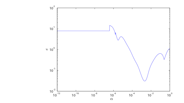
Figure 5: Maximum relative error against regularization parameter

From Figure 5, we can see that the maximum relative error reaches a minimum at $\alpha=10^{-2.673}\approx 2.12\times 10^{-3}$, which coincides with the suitable regularization parameter obtained by the L-curve. Hence, we know that the optimal regularization parameter can be given as the one corresponding to a regularized solution at the corner of the L-curve.

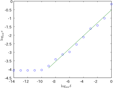
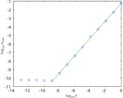
(a) (b)

Figure 6: (a) Maximum relative error and (b) the optimal regularization parameter against relative noise level

Figure 6 (a) shows the maximum relative error $e$ for the optimal regularized potential against the relative noise level $\delta$. The regression line in the interval $[-9,0]$ is expressed by $\log_{10}e=0.37951\log_{10}\delta-0.22672$. For the optimal regularized potential $u_{N}$, we have $e=O(\delta^{0.38})$ for $\delta\geq 10^{-9}$. Figure 6 (b) indicates the optimal regularization parameter $\alpha_{\rm opt}$ against the relative noise level $\delta$ and the regression line in the interval $[-9,0]$ given by $\log_{10}\alpha_{\rm opt}=1.0186\log_{10}\delta-1.2434$. From this numerical result, we can obtain the relation $\alpha_{\rm opt}=O(\delta)$ for $10^{-9}\leq\delta\leq 1$.

After setting the parameters $(R,M,N)$, we can obtain a suitable regularized solution based on the Tikhonov regularization and the L-curve. Now, our problem is how to choose suitable parameters $(R,M,N)$.

Figure 7 shows the maximum relative error against the number of collocation points. We know from this result that we need to take sufficiently many collocation points to obtain accurate solutions.

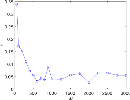
Figure 7: Maximum relative error against number of collocation points

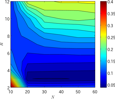
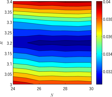
(a) (b)

Figure 8: Contour line of the maximum relative error against $(N,R)$ ($M=600$); (a) $(N,R)\in[10,60]\times[2,12]$, (b) $(N,R)\in[24,30]\times[3,3.4]$

Figure 8 shows the contour line of the maximum relative error $e$ against $(N,R)$ for the fixed number of collocation points $M=600$. Through this result, we know that the maximum relative error is roughly independent of the number of source points $N$ for the fixed radius $R$ of the circle where source points are distributed, and becomes large for large $R$. As a result, we know that the parameters $R\approx 3.2$ and $N\geq 25$ will yield a better regularized solution.

5.2 Irregular domain

As the next example, we assume the exact solution as same as the one in the previous example in an irregular domain enclosed by the boundary

$$x(\theta)=r(\theta)\cos\theta,\quad y(\theta)=r(\theta)\sin\theta,\qquad 0\leq\theta<2\pi$$

with the Cassini oval

$$r(\theta)=r(\theta;a,b)=a\sqrt{\cos 2\theta+\sqrt{(b/a)^{4}-\sin^{2}2\theta}},\qquad 0\leq\theta<2\pi$$ (13)

in the polar coordinates with $a=1,b=1.01$. It is easy to show that the unit outward normal to the boundary is expressed as

$${\boldsymbol{n}}(\theta)=\left(\frac{r^{\prime}(\theta)\sin\theta+r(\theta)\cos\theta}{\sqrt{(r^{\prime}(\theta))^{2}+r(\theta)^{2}}},\frac{-r^{\prime}(\theta)\cos\theta+r(\theta)\sin\theta}{\sqrt{(r^{\prime}(\theta))^{2}+r(\theta)^{2}}}\right).$$

We distribute collocation and source points along the boundary and the circle $(R\cos\theta,R\sin\theta)$ uniformly as similar as (12). Figure 9 shows the domain, the unit outward normal, the collocation and the source points for example.

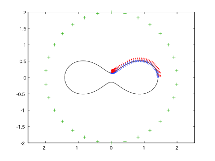
Figure 9: Domain and distribution of points ($(R,M,N)=(2,40,10)$)

The relative noise level of the Cauchy data is assumed to be $10\%$ ($\delta=0.1$). Let $(R,M,N)=(2,5200,30)$. The optimal regularization parameter can be found as $\alpha=2.3493\times 10^{-2}$ by using the L-curve. Figure 10 shows the regularized solution on the boundary with respect to the optimal regularization parameter.

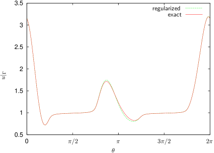
Figure 10: The regularized solution $u_{N}$ versus the exact $u$ ($10\%$ noise level; $(R,M,N)=(2,5200,30)$)

From the result, it is concluded that even if the boundary of the domain is complicated and the noise level of the Cauchy data is higher, the regularized solution is in very good agreement with the exact one.

5.3 Problems with singular points

We consider two problems whose solutions have singular points.

We first assume the exact solution

$$u(x,y)=\log\sqrt{(x-0.2)^{2}+y^{2}}-\log\sqrt{(x+0.2)^{2}+y^{2}}$$

in the annulus domain

$$\Omega=\{(x,y):0.5^{2}<x^{2}+y^{2}<1\}$$

with the outer and the inner boundaries

$$\Gamma_{\rm out}=\{(x,y):x^{2}+y^{2}=1\},\qquad\Gamma_{\rm in}=\{(x,y):x^{2}+y^{2}=0.5^{2}\}.$$

The exact solution $u$ has two singular points at $(x,y)=(-0.2,0),(0.2,0)$.

We now assume that the exact potential $u$ is unknown. From the Cauchy data given on the fourth part of the outer boundary $\Gamma_{\rm out}$, defined by

$$\Gamma_{1}:=\{(x,y):x^{2}+y^{2}=1,\ x>0,\ y>0\},$$

we identify a boundary value on the rest of the boundary $(\Gamma_{\rm out}\setminus\Gamma_{1})\cup\Gamma_{\rm in}$.

We distribute uniformly the collocation points $\{{\boldsymbol{x}}_{i}\}_{i=1}^{M}\subset\Gamma_{1}$. The source points $\{{\boldsymbol{\xi}}_{j}\}_{j=1}^{N}\subset\overline{\Omega}^{c}$ are uniformly distributed along two circles whose centers are 0 and radii are $R_{\rm out}$ and $R_{\rm in}$, respectively.

In the first case, the exact Cauchy data is assumed to be given. Let $(R_{\rm out},R_{\rm in},M,N)=(3.2,0.4,600,60)$ (Figure 11). Figure 12 shows the identified solution on the outer and the inner boundaries. We can see that the identified solution is in very good agreement with the exact one in spite of the solution with singular points.

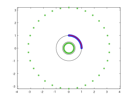
Figure 11: Domain and distribution of points ($(R_{\rm out},R_{\rm in},M,N)=(3.2,0.4,600,60)$)

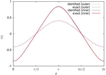
Figure 12: The regularized solution $u_{N}$ versus the exact $u$ (no noise)

In the second case, the relative noise level of the Cauchy data is assumed to be $5\%$ ($\delta=0.05$). Let $(R_{\rm out},R_{\rm in},M,N)=(3.2,0.2,5200,30)$ (Figure 13). The optimal regularization parameter can be found as $\alpha=6.3932\times 10^{-3}$ by using the L-curve. Figure 14 shows the regularized solution on the outer and the inner boundaries with respect to the optimal regularization parameter. From this result, we know that the regularized solution is acceptable.

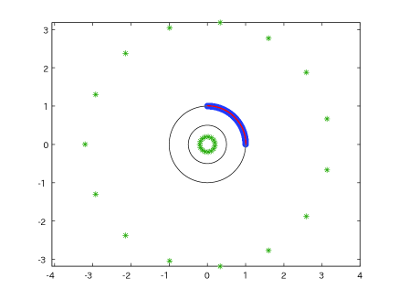
Figure 13: Domain and distribution of points ($(R_{\rm out},R_{\rm in},M,N)=(3.2,0.2,5200,30)$)

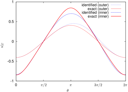
Figure 14: The regularized solution $u_{N}$ versus the exact $u$ ($5\%$ noise level)

As another example, we assume that the exact solution is given by

$$u(x,y)=\frac{x}{x^{2}+y^{2}}$$

in the same domain as above. The Cauchy data with $5\%$ noise level are prescribed on the same part of the boundary as above. Let $(R_{\rm out},R_{\rm in},M,N)=(3.2,0.05,5200,30)$. Figure 15 shows the regularized solution on the outer and the inner boundaries with respect to the optimal regularization parameter $\alpha=1.5088\times 10^{-3}$. The accuracy of the regularized solution is quite good.

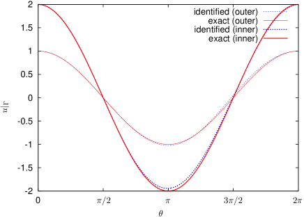
Figure 15: The regularized solution $u_{N}$ versus the exact $u$ ($5\%$ noise level)

6 Conclusions

We consider using MFS as the numerical method for the Cauchy problem of the Laplace equation. Since MFS is a messless method, we can easily treat a complicated boundary. This paper proposes a direct method instead of an iterative one. The Tikhonov regularization can find a stable solution. The L-curve automatically gives a suitable regularization parameter, which coincides with the optimal one shown in the numerical experiments. Hence, after setting the parameters $(R,M,N)$ the optimal regularized solution can be obtained quickly and automatically. Moreover, our numerical method can successfully solve even a problem whose solution has singular points.

The following is the guideline for choosing better parameters $(R,M,N)$: The collocation points should be distributed as many as possible compared with the source points. There is no value increasing the number of source points $N$. It is enough for $N\approx 30$ to obtain a better solution. The radius of the circle where source points are distributed should be small like $R\approx 3$, since the stability is more important than the accuracy in this inverse problem.

In conclusion, the numerical method proposed in this paper is applicable for solving a problem in a complicated domain with the Cauchy data that contains large noises even with a noise level of 10%. This method is also effective for solving even a problem with singular points.

References

- [1] Hansen PC. Analysis of discrete ill-posed problems by means of the L-curve. SIAM Review 1992; 34 (4): 561–580.
-
[2]
Hansen PC.
Regularization Tools, A Matlab Package for Analysis and
Solution of Discrete Ill-Posed Problems.
http://www2.imm.dtu.dk/~pch/Regutools/ - [3] Hansen PC. REGULARIZATION TOOLS: A Matlab package for analysis and solution of discrete ill-posed problems. Numerical Algorithms 1994; 6 (1): 1–35.
- [4] Wei T, Hon YC, Ling L. Method of fundamental solutions with regularization techniques for Cauchy problems of elliptic operators. Engineering Analysis with Boundary Elements 2007; 31: 373–385.
- [5] Hosoda Y, Kitagawa T. Optimal regularization for ill-posed problems by means of L-curve (in Japanese). Journal of the Japan Society for Industrial and Applied Mathematics 1992; 2 (1): 56–67.
- [6] Shigeta T. Mathematical aspects and numerical computations of an inverse boundary value identification using the adjoint method. Submitted.
- [7] Iijima K, Shirota K, Onishi K. A numerical computation for inverse boundary value problems by using the adjoint method. Contemporary Mathematics 2004; 348: 209–220.
- [8] Iijima K. Application of high order finite difference approximation as exponential interpolation. Theoretical and Applied Mechanics Japan 2004; 53: 239–247.
- [9] Onishi K, Kobayashi K, Ohura Y. Numerical solution of a boundary inverse problem for the Laplace equation. Theoretical and Applied Mechanics 1996; 45: 257–264.
- [10] Shirota K, Onishi K. Adjoint method for numerical solution of inverse boundary value and coefficient identification problems. Surveys on Mathematics for Industry 2005; 11: 43–93.
- [11] Bogomolny A. Fundamental solutions method for elliptic boundary value problems. SIAM Journal on Numerical Analysis 1985; 22 (4): 644–669.
- [12] Franzone, PC, Magenes E. On the inverse potential problem of electrocardiology Calcolo 1979; 16 (4): 459–538.
- [13] Mathon R, Johnston R L. The approximate solution of elliptic boundary-value problems by fundamental solutions. SIAM Journal on Numerical Analysis 1977; 14 (4): 638–650.
- [14] Katsurada M, Okamoto U. The collocation points of the fundamental solution method for the potential problem. Computers & Mathematics With Applications 1996; 31 (1): 123–137.
- [15] Ramachandran PA. Method of fundamental solutions: singular value decomposition analysis. Communication in Numerical Methods in Engineering 2002; 18: 789–891.