On the Throughput Allocation for Proportional Fairness in Multirate IEEE 802.11 DCF under General Load Conditions

Abstract

This paper presents a modified proportional fairness (PF) criterion suitable for mitigating the rate anomaly problem of multirate IEEE 802.11 Wireless LANs employing the mandatory Distributed Coordination Function (DCF) option. Compared to the widely adopted assumption of saturated network, the proposed criterion can be applied to general networks whereby the contending stations are characterized by specific packet arrival rates, $\lambda_{s}$, and transmission rates $R_{d}^{s}$.

The throughput allocation resulting from the proposed algorithm is able to greatly increase the aggregate throughput of the DCF while ensuring fairness levels among the stations of the same order of the ones available with the classical PF criterion. Put simply, each station is allocated a throughput that depends on a suitable normalization of its packet rate, which, to some extent, measures the frequency by which the station tries to gain access to the channel. Simulation results are presented for some sample scenarios, confirming the effectiveness of the proposed criterion.

I Introduction

Consider the IEEE802.11 Medium Access Control (MAC) layer [1] employing the DCF based on the Carrier Sense Multiple Access Collision Avoidance CSMA/CA access method. The scenario envisaged in this work considers $N$ contending stations; each station generates data packets with constant rate $\lambda_{s}$ by employing a bit rate, $R_{d}^{s}$, which depends on the channel quality experienced. In this scenario, it is known that the DCF is affected by the so-called performance anomaly problem [2]: in multirate networks the aggregate throughput is strongly influenced by that of the slowest contending station.

After the landmark work by Bianchi [3], who provided an analysis of the saturation throughput of the basic 802.11 protocol assuming a two dimensional Markov model at the MAC layer, many papers have addressed almost any facet of the behaviour of DCF in a variety of traffic loads and channel transmission conditions (see [4]-[5] and references therein). A current topic of interest in connection to DCF regards the allocation of throughput in order to mitigate the performance anomaly, while ensuring fairness among multirate stations.

With this background, let us provide a quick survey of the recent literature related to the problem addressed here. Paper [7] proposes a proportional fairness throughput allocation criterion for multirate and saturated IEEE 802.11 DCF by focusing on the 802.11e standard. In papers [8]-[11] the authors propose novel fairness criteria, which fall within the class of the time-based fairness criterion. Time-based fairness guarantees equal time-share of the channel occupancy irrespective of the station bit rate. Finally, paper [12] investigates the fairness problem in 802.11 multirate networks from a theoretical point of view.

A common hypothesis employed in the literature regards the saturation assumption. However, real networks are different in many respects. Traffic is mostly non-saturated, different stations usually operate with different loads, i.e., they have different packet rates, while the transmitting bit rate can also differ among the contending stations. In all these situations the common hypothesis, widely employed in the literature, that all the contending stations have the same probability of transmitting in a randomly chosen time slot, does not hold anymore. The aim of this paper is to present a proportional fairness criterion under much more realistic scenarios, especially when the packet rates among the station are different. As a starting point for the derivations that follow, we consider the bi-dimensional Markov model proposed in the companion paper [5], and present the necessary modifications in order to deal with the problem at hand.

The rest of the paper is organized as follows. Section II provides the necessary modifications to the Markov model proposed in [5]. For conciseness, we invite the interested reader to refer to [5] for further details about the bi-dimensional Markov model. The novel proportional fairness criterion is presented in Section III. Finally, simulation results of sample network scenarios are discussed in Section IV.

II Extension to the Markovian Model Characterizing the DCF

In a companion paper [5] (see also [4]), we derived a bi-dimensional Markov model for characterizing the behavior of the DCF under a variety of real traffic conditions, both non-saturated and saturated, with packet queues of small sizes, multirate setting, and considered the IEEE 802.11b protocol with the basic 2-way handshaking mechanism. As a starting point for the derivations which follow, we adopt the bi-dimensional model proposed in  [5], appropriately modified in order to account for the following scenario. In the investigated network, each station employs a specific bit rate, $R_{d}^{(s)}$, a different transmission packet rate, $\lambda_{s}$, transmits packets with size $PL^{(s)}$, and it employs a minimum contention window with size $W_{0}^{(s)}$, which can differ from the one specified in the IEEE 802.11 standard [1] (this is required for optimizing the aggregate throughput while guaranteeing fairness among the contending stations). For the sake of greatly simplifying the evaluation of the expected time slots required by the theoretical derivations that follow, we consider $N_{c}\leq N$ classes of channel occupancy durations. This assumption relies on the observation that in actual networks some stations might transmit data frames presenting the same channel occupancy.

The scenario at hand requires a number of modifications to the previous theoretical results derived in [5]. First of all, given the payload lengths and the data rates of the $N$ stations, the $N_{c}$ duration-classes are arranged in order of decreasing durations identified by the index $d\in\{1,\cdots,N_{c}\}$, whereby $d=1$ identifies the slowest class. Notice that in our setup a station is labelled as fast if it has a short channel occupancy. Furthermore, each station is identified by an index $s\in\{1,\cdots,N\}$, and it belongs to a unique duration-class. In order to identify the class of a station $s$, we define $N_{c}$ subsets $n(d)$, each of them containing the indexes of the $L_{d}=|n(d)|$ stations within $n(d)$, with $L_{d}\leq N,\forall d$ and $\sum_{d=1}^{N_{c}}L_{d}=N$. As an instance, $n(3)=\{1,5,8\}$ means that stations 1, 5, and 8 belong to the third duration-class identified by $d=3$, and $L_{d}=3$.

With this setup, the probability that the $s$-th station starts a transmission in a randomly chosen time slot is identified by $\tau_{s}$, and it can be obtained by solving the bidimensional Markov chain for the contention model of the $s$-th station [5]:

$$\small\tau_{s}=\frac{2(1-b_{I}^{(s)})(1-2P_{eq}^{(s)})}{(W_{0}^{(s)}+1)(1-2P_{eq}^{(s)})+W_{0}^{(s)}P_{eq}^{(s)}[1-(2P_{eq}^{(s)})^{m}]}$$ (1)

whereby $b_{I}^{(s)}$ is the stationary probability to be in an idle state modelling unloaded conditions, $W_{0}^{(s)}$ is the minimum contention window size of the $s$-th station, and $P^{(s)}_{eq}$ is the probability of equivalent failed transmission defined as $P^{(s)}_{eq}=1-(1-P_{e}^{(s)})(1-P_{col}^{(s)})=P^{(s)}_{col}+P^{(s)}_{e}-P^{(s)}_{e}\cdot P^{(s)}_{col}$, whereby $P^{(s)}_{col}$ and $P^{(s)}_{e}$ are, respectively, the collision and the packet error probabilities related to the $s$-th station. Given $\tau_{s}$ in (1), we can evaluate the aggregate throughput $S$ as follows:

$$S=\sum_{s=1}^{N}S_{s}=\sum_{s=1}^{N}\frac{1}{T_{av}}P_{s}^{(s)}\cdot(1-P_{e}^{(s)})\cdot PL^{(s)}$$ (2)

whereby $T_{av}$ is the expected time per slot, $PL^{(s)}$ is the packet size of the $s$-th station, and $P_{s}^{(s)}$ is the probability of successful packet transmission of the $s$-th station:

$$P_{s}^{(s)}=\tau_{s}\cdot\prod_{\begin{subarray}{c}j=1\\ j\neq s\end{subarray}}^{N}(1-\tau_{j})$$ (3)

The expected time per slot, $T_{av}$, can be evaluated by weighting the times spent by a station in a particular state with the probability of being in that state as already mentioned in [5]. Upon observing the basic fact that there are four kinds of time slots, namely idle time slot, successful transmission time slot, collision time slot, and channel error time slot, $T_{av}$ can be evaluated by adding the four expected slot durations:

$$T_{av}=T_{I}+T_{C}+T_{S}+T_{E}.$$ (4)

Let us evaluate $T_{I}$, $T_{C}$, $T_{S}$, and $T_{E}$.

Upon identifying with $\sigma$ an idle slot duration, and defining with $P_{TR}$ the probability that the channel is busy in a slot because at least one station is transmitting:

$$\small P_{TR}=1-\prod_{s=1}^{N}(1-\tau_{s})$$ (5)

the average idle slot duration can be evaluated as follows:

$$\small T_{I}=(1-P_{TR})\cdot\sigma$$ (6)

The average slot duration of a successful transmission, $T_{S}$, can be found upon averaging the probability $P_{s}^{(s)}$ that only the $s$-th tagged station is successfully transmitting over the channel, times the duration $T_{s}^{(s)}$ of a successful transmission from the $s$-th station:

$$\small T_{S}=\sum_{s=1}^{N}P_{s}^{(s)}\left(1-P_{e}^{(s)}\right)\cdot T_{S}^{(s)}$$ (7)

Notice that the term $(1-P_{e}^{(s)})$ accounts for the probability of packet transmission without channel induced errors.

Analogously, the average duration of the slot due to erroneous transmissions can be evaluated as follows:

$$\small T_{E}=\sum_{s=1}^{N}P_{s}^{(s)}\cdot P_{e}^{(s)}\cdot T_{E}^{(s)}$$ (8)

Let us focus on the evaluation of the expected collision slot, $T_{C}$. There are $N_{c}$ different values of the collision probability $P_{C}^{(d)}$, depending on the class of the tagged station identified by $d$. We assume that in a collision of duration $T_{C}^{(d)}$ (class-$d$ collisions), only the stations belonging to the same class, or to higher classes (i.e., stations whose channel occupancy is lower than the one of stations belonging to the tagged station indexed by $d$) might be involved.

In order to identify the collision probability $P_{C}^{(d)}$, let us first define the following three transmission probabilities ($P_{TR}^{C(d)},P_{TR}^{H(d)},P_{TR}^{L(d)}$) under the hypothesis that the tagged station belongs to the class $d$. Probability $P_{TR}^{L(d)}$ represents the probability that at least another station belonging to a lower class transmits, and it can be evaluated as

$$\small P_{TR}^{L(d)}=1-\prod_{i=1}^{d-1}\prod_{s\in n(i)}(1-\tau_{s})$$ (9)

Probability $P_{TR}^{H(d)}$ is the probability that at least one station belonging to a higher class transmits, and it can be evaluated as

$$\small P_{TR}^{H(d)}=1-\prod_{i=d+1}^{N_{c}}\prod_{s\in n(i)}(1-\tau_{s})$$ (10)

Probability $P_{TR}^{C(d)}$ represents the probability that at least a station in the same class $d$ transmits:

$$\small P_{TR}^{C(d)}=1-\prod_{s\in n(d)}(1-\tau_{s})$$ (11)

Therefore, the collision probability for a generic class $d$ takes into account only collisions between at least one station of class $d$ and at least one station within the same class (internal collisions) or belonging to higher class (external collisions). Hence, the total collision probability can be evaluated as:

$$\small P_{C}^{(d)}=P_{C}^{I(d)}+P_{C}^{E(d)}$$ (12)

whereby

$$\tiny P_{C}^{I(d)} = (1-P_{TR}^{H(d)})\cdot(1-P_{TR}^{L(d)})\cdot$$

$$\cdot\left[P_{TR}^{C(d)}-\sum_{s\in n(d)}\tau_{s}\prod_{j\in n(d),j\neq\ s}(1-\tau_{j})\right]$$

represents the internal collisions between at least two stations within the same class $d$, while the remaining are silent, and

$$\small P_{C}^{E(d)}=P_{TR}^{C(d)}\cdot P_{TR}^{H(d)}\cdot(1-P_{TR}^{L(d)})$$ (14)

concerns to the external collisions with at least one station of class higher than $d$.

Finally, the expected duration of a collision slot is:

$$\small T_{C}=\sum_{d=1}^{N_{c}}P_{C}^{(d)}\cdot T_{C}^{(d)}$$ (15)

Constant time durations $T_{S}^{(s)}$, $T_{E}^{(s)}$ and $T_{C}^{(d)}$ are defined in a manner similar to [5] with the slight difference that the first two durations are associated to a generic station $s$, while the latter is associated to each duration class, which depends on the combination of both payload length and data rate of the station of class $d$.

II-A Traffic Model

The employed traffic model assumes a Poisson distributed packet arrival process, where interarrival times between two packets are exponentially distributed with mean $1/\lambda$. In order to greatly simplify the analysis, we consider small queue (i.e., $KQ\rightarrow 1$, where $KQ$ is the queue size expressed in number of packets). In order to account for the station traffic, the Markov model employs two probabilities, $q$ and $P_{I,0}$, defined as in [5]. Briefly, non-saturated traffic is accounted for by a new state labelled $I$, which considers the following two situations: 1) After a successful transmission, the queue of the transmitting station is empty. This event occurs with probability $(1-q^{(t)})(1-P_{eq}^{(t)})$, whereby $q^{(t)}$ is the probability that there is at least one packet in the queue after a successful transmission. 2) The station is in an idle state with an empty queue until a new packet arrives in the queue. Probability $P_{I,0}^{(t)}$ represents the probability that while the station resides in the idle state $I$ there is at least one packet arrival, and a new backoff procedure is scheduled. In our analysis, each station has its own traffic; therefore, for the $t$-th tagged station we have $q^{(t)}$ and $P^{(t)}_{I,0}$, which can be evaluated as $q^{(t)}=1-e^{-\lambda^{(t)}\cdot T_{av}}$ and $P^{(t)}_{I,0}=1-e^{-\lambda^{(t)}\cdot T^{-t}_{av}}$, respectively. Notice that $q^{(t)}$ and $P^{(t)}_{I,0}$ stem from the fact that, for exponentially distributed interarrival times with mean $1/\lambda^{(t)}$, the probability of having at least one packet arrival during time $T$ is equal to $1-e^{-\lambda^{(t)}\cdot T}$. Concerning $P^{(t)}_{I,0}$, the average time spent by the system in the idle state, i.e., $T^{-t}_{av}$, is evaluated as $T_{av}$ in (4) except for the fact that the tagged station is not considered in the evaluation of the expected times defining $T_{av}$. On the other hand, $q^{(t)}$ is calculated over the entire average time slot duration, which also considers the tagged station.

III The Proportional Fairness Throughput Allocation Algorithm

This section presents the novel throughput allocation criterion along with a variation that proved to be useful in relation to the packet rate of the slowest station in the network. In order to face the fairness problem in the most general scenario, i.e., multirate DCF and general station loading conditions, we propose a novel proportional fairness criterion (PFC) by starting from the PCF defined by Kelly in [13], and employed in [7] in connection to proportional fairness throughput allocation in multirate and saturated DCF operations.

In the proposed model, the traffic of each station is characterized by the packet arrival rate $\lambda_{s}$, which depends mainly on the application layer. Upon setting $\lambda_{max}$ equal to the maximum value among the packet rates $\lambda_{1},\ldots,\lambda_{N}$ of the $N$ contending stations, consider the following modified PFC:

$$\begin{array}[]{ll}\mbox{max}&U=U(S_{1},\cdots,S_{N})=\sum_{s=1}^{N}\frac{\lambda_{s}}{\lambda_{max}}\cdot\log(S_{s})\\ \mbox{subject to}&S_{s}\in[0,S_{s,m}],~{}s=1,\ldots,N\end{array}$$ (16)

whereby $S_{s}$ is the throughput of the $s$-th station, and $S_{s,m}$ is its maximum value, which equal the station bit rate $R_{d}^{(s)}$. In our scenario, the individual throughputs, $S_{s}$, are interlaced because of the interdependence of the probabilities involved in the transmission probabilities $\tau_{s},\forall s=1,\ldots,N$. For this reason, we reformulate the maximization problem in order to find the $N$ optimal values of $\tau_{s}$ for which the cost function in (16) gets maximized. Put simply, upon starting from the optimum $\tau_{s}^{*}$, we obtain the set of parameters of each station such that optimal point is attained.

Due to the compactness of the feasible region $S_{s}\in[0,S_{s,m}],\forall s$, the maximum of $U(S_{1},\cdots,S_{N})$ can be found among the solutions of $\nabla U=\left(\frac{\partial U}{\partial\tau_{1}},\cdots,\frac{\partial U}{\partial\tau_{N}}\right)=0.$ After some algebra (the proof is reported in the paper [6]), the solutions can be written as:

$$\frac{\lambda_{j}}{\lambda_{max}}\frac{1}{\tau_{j}}-\frac{1}{1-\tau_{j}}\sum_{k=1,k\neq j}^{N}\frac{\lambda_{k}}{\lambda_{max}}=\frac{C}{T_{av}}\frac{\partial T_{av}}{\partial\tau_{j}},\quad\forall j=1,\ldots,N$$ (17)

whereby $C=\sum_{i=0}^{N}\frac{\lambda_{i}}{\lambda_{max}}$, and $T_{av}$ is a function of $\tau_{1},\cdots,\tau_{N}$ as noted in (4).

Due to the presence of $T_{av}$, a closed form of the maximum of $U(S_{1},\cdots,S_{N})$ cannot be found. Notice that it is quite difficult to derive the contribution of the partial derivative of $T_{av}$ on $\tau_{j}$, especially when $N\gg 1$, because of the huge number of network parameters belonging to different stations. The definition of $T_{av}$ in (4) is composed by four different terms, anyone of which includes the whole set of $\tau_{s}$, $\forall s$. In order to overcome this problem, we first obtain the optimal values $\tau_{s}^{*},\forall s$ from (17) by means of Mathematica. Then, we choose the value of the minimum contention window size, $W^{(s)}_{0}$, by equating the optimizing $\tau_{s}^{*}$ to (1) for any $s$.

The results of the optimization problem (16) will be denoted by the acronym LPF in the following.

Let us derive some observations on the proposed throughput allocation algorithm by contrasting it to the classical PF algorithm. Upon employing the classical PF method, a throughput allocation is proportionally fair if a reduction of $x\%$ of the throughput allocated to one station is counterbalanced by an increase of more than $x\%$ of the throughputs allocated to the other contending stations. The key observation in our setup can be summarized as follows. Consider the two stations above with packet rates $\lambda_{1}=50~{}\textrm{pkt/s}$ and $\lambda_{2}=100~{}\textrm{pkt/s}$, respectively. The ratio $\lambda_{1}/\lambda_{2}$ can be interpreted as the frequency by which the first station tries to get access to the channel relative to the other station. By doing so, in our setup a throughput allocation is proportionally fair if, for instance, a reduction of $20\%$ of the throughput allocated to the first station, which has a relative frequency of $1/2$, is counterbalanced by an increase of more than $40\%$ of the throughput allocated to the second station. In a scenario with multiple contending stations, the relative frequency is evaluated with respect to the station with the highest packet rate in the network, which gets unitary relative frequency.

Based on extensive analysis, we found that the optimization problem (16) sometimes yields throughput allocations that cannot be actually managed by the stations. As a reference example, assume that, due to the specific channel conditions experienced, the first station has a bit rate equal to $1$ Mbps and needs to transmits $200~{}\textrm{pkt/s}$. Given a packet size of $1024$ bytes, that is $8192$ bits, the first station would need to transmit $8192\times 200~{}\textrm{bps}\approx 1.64\textrm{Mbps}$ far above the maximum bit rate decided at the physical layer. In this scenario, such a station could not send over the channel a throughput greater than 1Mbps. The same applies to the other contending stations in the network experiencing similar conditions. In order to face this issue, we considered the following optimization problem

$$\begin{array}[]{ll}\mbox{max}&\sum_{s=1}^{N}\frac{\lambda^{*}_{s}}{\lambda^{*}_{max}}\cdot\log(S_{s})\\ \mbox{over}&S_{s}\in[0,S_{s,m}],~{}s=1,\ldots,N\end{array}$$ (18)

whereby, $\forall s=1,\ldots,N$, it is

$$\lambda^{*}_{s}=\left\{\begin{array}[]{ll}\lambda_{s}&\textrm{if}~{}\lambda_{s}\cdot PL^{(s)}\cdot 8\leq R_{d}^{(s)}\\ \frac{R_{d}^{(s)}}{8\cdot PL^{(s)}}&\textrm{if}~{}\lambda_{s}\cdot PL^{(s)}\cdot 8>R_{d}^{(s)}\end{array}\right.$$

and $\lambda^{*}_{max}=\max_{s}\lambda^{*}_{s}$. The allocation problem in (18), solved as for the LPF in (16), guarantees a throughput allocation which is proportional to the frequency of channel access of each station relative to their actual ability in managing such traffic. The results of the optimization problem (18) will be denoted by the acronym MLPF in the following section.

IV Simulation Results

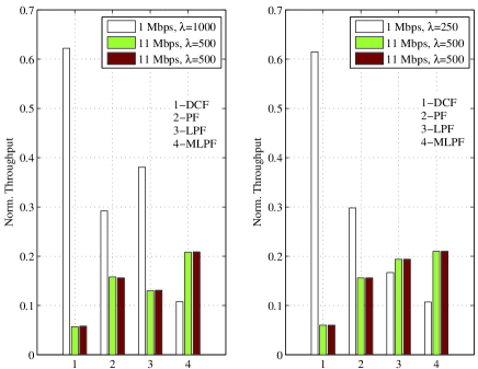
Figure 1: Simulated normalized throughput achieved by three contending stations upon employing 1) a classical DCF; 2) DCF with PF allocation; 3) DCF optimized as noted in (16); and 4) DCF optimized with the criterion MLPF. Left and right plots refer to scenarios A and B, respectively.

This section presents some preliminary simulation results obtained for two network scenarios optimized with the fairness criteria proposed in the previous section. Typical MAC layer parameters for IEEE802.11b [1] have been used for performance validation. Due to space limitations, we invite the interested reader to consult [5] for a list of the network parameters employed here as well as for the details about the employed simulator. Moreover, further results on the behaviour of the proposed criteria are available on the work [6].

The first investigated scenario, namely A, considers a network with $3$ contending stations. Two stations transmit packets with rate $\lambda=500~{}\textrm{ pkt/s}$ at $11$ Mbps. The payload size, assumed to be common to all the stations, is $PL=1028$ bytes. The third station has a bit rate equal to 1Mbps and a packet rate $\lambda=1000~{}\textrm{ pkt/s}$. The simulated normalized throughput achieved by each station in this scenario is depicted in the left subplot of Fig. 1 for the following four setups. The three bars labelled 1-DCF represent the normalized throughput achieved by the three stations with a classical DCF. The second set of bars, labelled 2-PF, identifies the simulated normalized throughput achieved by the DCF optimized with the PF criterion [7, 13], whereby the actual packet rates of the stations are not considered. The third set of bars, labelled 3-LPF, represents the normalized throughput achieved by the three stations when the allocation problem (16) is employed. Finally, the last set of bars, labelled 4-MLPF, represents the simulated normalized throughput achieved by the contending stations when the CW sizes are optimized with the modified fairness criterion. Notice that the throughput allocations guaranteed by LPF and MLPF improve over the classical DCF. When the station packet rate is considered in the optimization framework, a higher throughput is allocated to the first station presenting the maximum value of $\lambda$ among the considered stations. However, the highest aggregate throughput is achieved when the allocation is accomplished with the optimization framework 4-MLPF. The reason for this behaviour is related to the fact that the first station requires a traffic equal to $8.22\textrm{ Mbps}=10^{3}\textrm{ pkt/s}\cdot 1028\textrm{ bytes/pkt}\cdot 8\textrm{ bits/pkt}$, which is far above the maximum traffic ($1\textrm{ Mbps}$) that the station would be able to deal with in the best scenario. In this respect, the criterion MLPF results in better throughput allocations since it accounts for the real traffic that the contending station would be able to deal with in the specific scenario at hand.

Similar considerations can be drawn from the results shown in the right subplot of Fig. 1 (related to scenario B), whereby in the simulated scenario the two fastest stations are also characterized by a packet rate greater than the one of the slowest station. Notice that the optimization framework 3-LPF is able to guarantee improved aggregate throughput with respect to both the non-optimized DCF and the classical PF algorithms.

The aggregate throughput achieved in the two investigated scenarios are noted in Table I, whereby we also show the fairness Jain’s index [14] evaluated on the normalized throughputs noted in the subplots of Fig. 1. It is worth noticing that the proposed throughput allocation criteria are able to guarantee either improved aggregate throughput, and improved fairness among the contending stations over both the classical DCF and the PF algorithm. Moreover, notice that the fairness index and the aggregate throughput of both DCF and PF do not change in the two scenarios, since they do not account for the actual packet rates that the contending stations need to transmit over the channel.

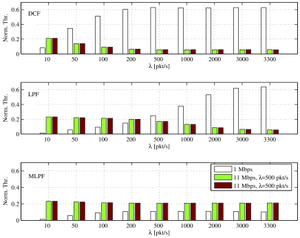
Figure 2: Simulated normalized throughput achieved by three contending stations as a function of the packet rate of the slowest station in DCF, LPF and MLPF modes.

For the sake of investigating the behaviour of the proposed allocation criteria as a function of the packet rate of the slowest station, we simulated the throughput allocated to a network composed by three stations, whereby the slowest station, transmitting at 1Mbps, presents an increasing packet rate in the range 10$-$3300 pkt/s. The other two stations transmit packets at the constant rate $\lambda=500$ pkt/s at 11 Mbps. The simulated throughput of the three contending stations is shown in the three subplot of Fig. 2 for the unoptimized DCF, as well as for the two criteria LPF and MLPF. Some considerations are in order. Let us focus on the throughput of the DCF (uppermost subplot in Fig. 2). As far as the packet rate of the slowest station increases, the throughput allocated to the fastest stations decreases quite fast because of the performance anomaly of the DCF [2]. The three stations reach the same throughput when the slowest station presents a packet rate equal to $500\textrm{pkt/s}$, corresponding to the one of the other two stations. From $\lambda=500\textrm{pkt/s}$ all the way up to 3300 pkt/s, the throughput of the three stations do not change anymore, since all the stations have a throughput imposed by the slowest station in the network. Let us focus on the results shown in the other two subplots of Fig. 2, labelled LPF and MLPF, respectively. A quick comparison among these three subplots in Fig. 2 reveals that the allocation criterion MLPF guarantees improved aggregate throughput for a wide range of packet rates of the slowest station, greatly mitigating the rate anomaly problem of the classical DCF operating in a multirate setting. In terms of aggregate throughput, the best solution is achieved with the criterion MLPF.

TABLE I: Jain’s Fairness Index and Aggregate Throughput S

Scenarios in Fig. 1		1-DCF	2-PF	3-LPF	4-MLPF
A	Jain’s Index	0.460	0.909	0.766	0.9317
	S [Mbps]	1.89	3.74	3.25	4.69
B	Jain’s Index	0.467	0.902	0.995	0.9290
	S [Mbps]	1.93	3.73	4.43	4.72

References

- [1] IEEE Standard for Wireless LAN Medium Access Control (MAC) and Physical Layer (PHY) Specifications, November 1997, P802.11
- [2] M. Heusse, F. Rousseau, G. Berger-Sabbatel, and A. Duda, “Performance anomaly of 802.11b” In Proc. of IEEE INFOCOM 2003, pp. 836-843.
- [3] G. Bianchi, “Performance analysis of the IEEE 802.11 distributed coordination function”, IEEE JSAC, Vol.18, No.3, March 2000.
- [4] F. Daneshgaran, M. Laddomada, F. Mesiti, and M. Mondin, “Modelling and analysis of the distributed coordination function of IEEE 802.11 with multirate capability”, In Proc. of IEEE WCNC 2008, March 2008.
-
[5]
F. Daneshgaran, M. Laddomada, F. Mesiti, and M. Mondin,
“On the behavior of the distributed coordination function of IEEE
802.11 with multirate capability under general transmission
conditions”, Submitted to IEEE Trans. on Wireless
Communications, October 2007, Available online at
http://arxiv.org/abs/0710.3955v1 -
[6]
F. Daneshgaran, M. Laddomada, F. Mesiti, and M. Mondin,
“A Novel Throughput Allocation Scheme for Proportional Fairness
in Multirate IEEE 802.11 DCF under General Load Conditions”, In preparation, 2008, Available online at
http://arxiv.org. - [7] A. Banchs, P. Serrano, and H. Oliver, “Proportional fair throughput allocation in multirate IEEE 802.11e wireless LANs”, Wireless Networks, Vol 13, No. 5, pages 649-662, May 2007.
- [8] I. Tinnirello and S. Choi, “Temporal fairness provisioning in multi-rate contention-based 802.11e WLANs”, In Proc. of Sixth IEEE Int. Symp. on WoWMoM 2005, pp.220 - 230, June 2005.
- [9] G. Tan and J. Guttag, “Time-based fairness improves performance in multi-rate WLANs”, USENIX Annual Technical Conference, June 27-July 2, 2004, Boston, MA, USA.
- [10] A.V. Babu, L. Jacob, and V. Brijith, “A novel scheme for achieving time based fairness in IEEE 802.11 multirate wireless LANs”, In Proc. of 13th IEEE International Conference on Networks 2005, Vol.1, pp.16-18, November 2005.
- [11] T. Joshi, A. Mukherjee, Y. Yoo, and D. P. Agrawal, “Air time fairness for IEEE 802.11 multi rate networks”, IEEE Trans. on Mobile Computing, to appear 2008.
- [12] A.V. Babu and L. Jacob, “Fairness analysis of IEEE 802.11 multirate wireless LANs”, IEEE Trans. on Vehicular Technology, Vol.56, No.5, pp.3073-3088, Sept. 2007.
- [13] F. Kelly, “Charging and rate control for elastic traffic”, European Trans. on Telecommunications, Vol.8, No.1, pp.33-37, January 1997.
- [14] R. Jain, D. Chiu, and W. Hawe, “A quantitative measure of fairness and discrimination for resource allocation in shared computer systems”, Digital Equip. Corp., Littleton, MA, DEC Rep., DEC-TR-301, September 1984.
- [15] G. Bolch, S. Greiner, H. de Meer, and K.S. Trivedi, Queueing Networks and Markov Chains, Wiley-Interscience, 2nd edition, 2006.