Thermodynamic versus Topological Phase Transitions: Cusp in the Kertész Line

Abstract

We present a study of phase transitions of the mean–field Potts model at (inverse) temperature $\beta$, in presence of an external field $h$. Both thermodynamic and topological aspects of these transitions are considered. For the first aspect we complement previous results and give an explicit equation of the thermodynamic transition line in the $\beta$–$h$ plane as well as the magnitude of the jump of the magnetization (for $q\geqslant 3)$. The signature of the latter aspect is characterized here by the presence or not of a giant component in the clusters of a Fortuin–Kasteleyn type representation of the model. We give the equation of the Kertész line separating (in the $\beta$–$h$ plane) the two behaviours. As a result, we get that this line exhibits, as soon as $q\geqslant 3$, a very interesting cusp where it separates from the thermodynamic transition line.

1 Introduction

In [1], Kertész pointed out that a very interesting phenomenon arises in the Ising model subject to an external field. The so-called Coniglio–Klein droplets [2] associated to Fortuin–Kasteleyn clusters [3] have a whole percolation transition line extending from the Curie point to infinite fields. This seems, at first sight in contradiction with the fact that on the other hand, thermodynamics quantities do not have any singularities in any of their derivatives (with respect to the temperature or the field) as soon as the field is non–zero. But, as Kertész already mentioned:

However, we emphasize that the suggested picture is not in contradiction with the non existence of singularities in the thermodynamic quantities because the total free energy remains analytic.

Indeed in such a model, the criticality can be specified in two different ways: the thermodynamic criticality associated to the thermodynamic limit of the bulk free energy and the geometric criticality associated in the same limit to another lower order free energy.

Since then, the Kertész line has remained the subject of interests over the years for various models of statistical mechanics. In particular, it has been considered recently in [4] within the Potts’ model on the regular lattice $\mathbb{Z}^{d}$. There it was found, that, in dimension $d=2$, the whole thermodynamic first order transition line (when such first order behavior is present in the system) coincides with the Kertész line. The latter is also first order in the corresponding range of values of temperature and field.

The aim of this letter is to present a study of such a model when the underlying lattice is the complete graph with $n$ vertices. In this case the model is called mean–field or Curie–Weiss Potts model.

2 The model

To introduce the Potts model on the complete graph we attach to the sites $i=1,\ldots,n$ of the graph, spin variables $\sigma_{i}$ that take values in the set $\{1,\ldots,q\}$. The model at temperature $T=1/\beta$ and subject to an external field $H=h/\beta$ is then defined by the Gibbs measure

$$\mu_{\operatorname{Potts}}(\boldsymbol{\sigma})=\frac{1}{Z_{\operatorname{Potts}}}\prod_{i<j}e^{(\beta/n)(\delta_{\sigma_{i},\sigma_{j}}-1)}\prod_{i}e^{h\delta_{\sigma_{i},1}}$$ (1)

over spins configurations $\boldsymbol{\sigma}$. Here, $Z_{\operatorname{Potts}}$ denotes the partition function, the indices $i,j$ runs over the set $\{1,\ldots,n\}$, and $\delta$ is the Kronecker symbol. The critical (thermodynamic) behaviour of this model is well known [5], [6], [7], and mainly governed by the mean field equation

$$h=-\beta s+\ln\frac{1+(q-1)s}{1-s}$$ (2)

Namely, when $h=0$, there exists a threshold value

$$\beta_{c}^{(q)} = 2\hskip 10.00002pt\operatorname{for}\hskip 10.00002ptq=2$$ (3)

$$\beta_{c}^{(q)} = 2\frac{q-1}{q-2}\ln(q-1)\hskip 10.00002pt\operatorname{for}\hskip 10.00002ptq\geqslant 3$$ (4)

such that the system exhibits at $\beta_{c}^{(q)}$ a continuous transition when $q=2$, and a first order transition when $q\geqslant 3$. When $h>0$, no transition occurs if $q=2$, while as soon as $q\geqslant 3$ a first order transition line appears for which the microcanonical free energy of the model has two minima associated with two different solutions of the mean field equation [5], [7].

To study the behaviour of clusters previously mentioned, we turn to the Edwards–Sokal joint measure [8] given by

$$\mu_{\operatorname{ES}}(\boldsymbol{\sigma},\boldsymbol{\eta})=\frac{1}{Z_{\operatorname{ES}}}\prod_{i<j}[e^{-\frac{\beta}{n}}(1-\eta_{ij})+(1-e^{-\frac{\beta}{n}})\eta_{ij}\delta_{\sigma_{i},\sigma_{j}}]\\ \times\prod_{i}e^{h\delta_{\sigma_{i},1}}$$ (5)

where the edges variables $\eta_{ij}$ belong to $\{0,1\}$.

Notice that when $h=\infty$, all $\sigma_{i}=1$. This means that we open edges ($\eta_{ij}=1$) with probability (w.p.) $p=1-e^{-\beta/n}$ and close edges ($\eta_{ij}=0$) w.p. $e^{-\beta/n}$. This is nothing else than the well known Erdös–Rényi random graph $\mathcal{G}(n,p)$ [9]. This random graph is known to exhibit a (topological) transition at $\beta=1$ such that with probability tending to $1$ as $n\to\infty$:

1. for $\beta<1$ all components of open edges are at most of order $\ln n$.

2. at $\beta=1$ a giant component of order $n^{2/3}$ appears.

3. for $\beta>1$ this giant component becomes of order $s^{\ast}n$ where $s^{\ast}$ is the largest root of the mean field equation (2) with $q=1$ and $h=0$.

We refer the reader to [10], [11] for detailed discussions and proofs (see also [12] for a new approach of this transition).

Notice also that, on the other hand, when $h=0$, the marginal of the ES measure over the edges variables is the random cluster model:

$$\mu_{\operatorname{RC}}(\boldsymbol{\eta})=\frac{1}{Z_{\operatorname{RC}}}\prod_{i<j}e^{-(\beta/n)(1-\eta_{ij})}(1-e^{-\beta/n})^{\eta_{ij}}q^{C(\boldsymbol{\eta})}$$ (6)

where $C(\boldsymbol{\eta})$ denotes the number of connected components (including isolated sites) of open edges of the configuration $\boldsymbol{\eta}$. For $q=1$, this model again reduces to $\mathcal{G}(n,p)$ with $p$ as before. A refined study of the random cluster model (6) is given in [13] (see also [14], [15]). There, it is shown that with the threshold value $\beta_{c}^{(q)}$, given by (3) for $0<q\leqslant 2$ and by (4) for $q>2$, then with probability tending to $1$ as $n\to\infty$:

1. if $\beta<\beta_{c}^{(q)}$, the largest component (of open edges) of $\mu_{\operatorname{RC}}$ is of order $\ln n$.

2. if $\beta>\beta_{c}^{(q)}$, the largest component of $\mu_{\operatorname{RC}}$ is of order $s_{0}n$, where $s_{0}>0$ is the largest root of the mean field equation (2) with $h=0$.

3. if $\beta=\beta_{c}^{(q)}$ and $0<q\leqslant 2$, $\mu_{\operatorname{RC}}$ has largest component of order $n^{2/3}$.

4. if $\beta=\beta_{c}^{(q)}$ and $q>2$, $\mu_{\operatorname{RC}}$ is either as in a) or as in b).

According to these results, it is natural to expect for model $\mu_{\operatorname{ES}}$ (and its marginal over the edges variables), a Kertész line $h_{K}(\beta)$, interpolating betwen $h_{K}(1)=\infty$ and $h_{K}(\beta_{c}^{(q)})=0$, that signs the emergence of a giant component in the open edges of the configuration $\boldsymbol{\eta}$.

To study this line, it is convenient to consider a colored version of the Edwards–Sokal formulation. Namely, whenever the endpoints $ij$ of a given edge are occupied by a spin of color $a$, we label the variable $\eta_{ij}$ with a superscript indicating the color. For a spin configuration $\boldsymbol{\sigma}$, let $n_{a}(\boldsymbol{\sigma})$ be the number of sites occupied by spins of color $a=1,\ldots,q$. We then relabel the variables $\eta_{ij}^{a}$ by $\eta_{kl}^{a}:k<l\in\{1,\dots,n_{a}(\boldsymbol{\sigma})\}$. This means that, for any pairs $i<j\in\{1,\dots,n_{a}(\boldsymbol{\sigma})\}$, we open an edge $\eta_{ij}^{a}=1$ w.p. $1-e^{-\beta/n}$, and close this edge $\eta_{ij}^{a}=0$ w.p. $e^{-\beta/n}$. All the other edges between two sites of different colors are closed. The resulting measure becomes

$$\mu_{\operatorname{CES}}(\boldsymbol{\sigma},\boldsymbol{\eta}^{1},\ldots,\boldsymbol{\eta}^{q})=\frac{e^{hn_{1}(\boldsymbol{\sigma})}}{Z_{\operatorname{CES}}}\prod_{a=1}^{q}e^{\beta n_{a}(\boldsymbol{\sigma})(n_{a}(\boldsymbol{\sigma})-1)/2n}\\ \times\prod_{i<j\in\{1,\ldots,n_{a}(\boldsymbol{\sigma})\}}[e^{-\beta/n}(1-\eta^{a}_{ij})+(1-e^{-\beta/n})\eta^{a}_{ij}]$$ (7)

By summing over the spins variables, we get the following Colored–Random–Cluster model

$$\mu_{\operatorname{CRC}}(\boldsymbol{\eta}^{1},\ldots,\boldsymbol{\eta}^{q})=\frac{1}{Z_{\operatorname{CRC}}}\sum_{n_{1}+\cdots+n_{q}=n}Z(n_{1},\ldots,n_{q})\\ \times\prod_{a=1}^{q}\prod_{i<j\in\{1,\ldots,n_{a}\}}[e^{-\beta x_{a}/n_{a}}(1-\eta^{a}_{ij})+(1-e^{-\beta x_{a}/n_{a}})\eta^{a}_{ij}]$$ (8)

where $x_{a}=n_{a}/n$ are the densities of the colors and

$$Z(n_{1},\ldots,n_{q})=\frac{n!}{n_{1}!\cdots n_{q}!}\ e^{hn_{1}}\prod_{a=1}^{q}e^{\beta n_{a}(n_{a}-1)/2n}$$ (9)

This colored random cluster model can be thought as follows. Given a partition $n_{1},\ldots,n_{q}$ of $n$, we have $q$ classical Erdös–Rényi random graphs where the edges are open w.p. $1-e^{-\beta x_{a}/n_{a}}$. The asymptotic behavior of the partition as $n\rightarrow\infty$ will be determined by minimizing the free energy

$$f(x_{1},\ldots,x_{q})=-\lim_{n\rightarrow\infty}\frac{1}{n}\ln Z(n_{1},\ldots,n_{q})$$ (10)

where the limit is taken in such a way that $n_{a}/n\rightarrow x_{a}$.

Notice that, up to a normalizing factor, $Z(n_{1},\ldots,n_{q})$ is the microcanonical partition function of the Potts model (1) restricted to configurations such that the number of spins of color $a$ is fixed to $n_{a}$. This will give the thermodynamic behavior of the system and will determine the densities $x_{a}$. Once this is done the topological properties can be analysed by using the known properties of classical random graphs. Due to the presence of the field or using the symmetry of colors for vanishing field, we will pick up the first color. Then, the threshold value of the (topological) transition will be given by

$$\beta_{K}x_{1}=1$$ (11)

For $\lambda=\beta x_{1}>1$ a giant component will appears, with size of order $\Theta_{x_{1}}n\equiv\theta_{\beta x_{1}}x_{1}n$ where $\theta_{\lambda}$ is the largest root of the mean field equation

$$\lambda\theta=-\ln(1-\theta)$$ (12)

Let us briefly recall the minimization procedure for (10). By Stirling’s formula, we have $n!/n_{1}!\cdots n_{q}!\sim\prod_{a=1}^{a}e^{x_{a}\ln x_{a}}$ at the leading order in $n$, giving

$$f(x_{1},\ldots,x_{q})=\sum_{a=1}^{a}x_{a}\ln x_{a}-\frac{\beta}{2}\sum_{a=1}^{a}x_{a}^{2}-hx_{1}$$ (13)

The minima of this function can be parametrised by a real number $s$, $0\leqslant s\leqslant 1$, such that the minimizing vector $(x_{1},\ldots,x_{q})$ have the components

$$x_{1} = \frac{1+(q-1)s}{q}$$ (14)

$$x_{a} = \frac{1-s}{q}\hskip 10.00002pta=2,\ldots,q$$ (15)

(with arbitrary order for $h=0$).

The free energy (13) then takes the form

$$f(s)=\frac{1+(q-1)s}{q}\ln(1+(q-1)s)\\ +\frac{q-1}{q}(1-s)\ln(1-s)-\beta\frac{(q-1)}{2q}s^{2}\\ -h\frac{1+(q-1)s}{q}-\frac{\beta}{2q}-\ln q$$ (16)

The minimizers have to be found among the solutions of the mean field equation (2) obtained by differentiating $f$ with respect to $s$. Note that by taking into account (14) the condition (11) becomes

$$\beta_{K}\frac{1+(q-1)s}{q}=1$$ (17)

3 Results

Let us first consider the case $q=2$.

When $h=0$, the mean field equation (2) has a unique solution $s_{0}=0$ for $\beta\leqslant 2$, and a unique solution $s_{0}>0$ for $\beta>2$. Inserting $s_{0}$ into (17), we obtain that the giant component appears at $\beta_{K}^{(2)}=2$, getting thus $\beta_{K}^{(2)}=\beta_{c}^{(2)}$. There, this component is of order $n^{2/3}$. For $\beta>2$, $\beta x_{1}(s_{0})>1$, and we are in the supercritical regime with a giant component of order $\Theta_{x_{1}(s_{0})}n$. For $\beta<2$, $\beta x_{1}(s_{0})<1$, and we are in the subcritical regime with components of order at most $\ln n$.

When $h>0$,  the mean field equation has a unique solution $s_{0}>0$ for any $\beta$ (no thermodynamic transition occurs). The transition line $\beta_{K}^{(2)}(h)$, or equivalently $h_{K}^{(2)}(\beta)$, is obtained by eliminating $s$ between (2) and (17). This Kertész line is given by

$$h^{(2)}_{K}(\beta)=\beta-2-\ln(\beta-1)$$ (18)

On this line, the largest component is of order $n^{2/3}$. For $h<h_{K}$, the largest component is of order $\ln n$, while for $h>h_{K}$, the largest component is of order $\Theta_{x_{1}(s_{0})}n$.

Let us then consider the case $q\geqslant 3$. We have now a thermodynamic transition line

$$h_{T}(\beta)=-\beta\frac{q-2}{2(q-1)}+\ln(q-1),\hskip 10.00002pt\beta_{0}\leqslant\beta\leqslant\beta_{c}^{(q)}$$ (19)

with endpoints

$$(\beta_{0}=4\frac{q-1}{q},h_{0}=-2\frac{q-2}{q}+\ln(q-1)),\hskip 10.00002pt(\beta_{c}^{(q)},0)$$ (20)

As previously mentionned, the thermodynamic transition has been already established in [7], for a curve with endpoints (20). To show that the thermodynamic curve is the straight line (19) we observe, on $h_{T}$ the free energy (16) has the symmetry $f(s)=f(\frac{q-2}{q-1}-s)$ with $s\in[0,\frac{q-2}{q-1}]$, see Fig. 1.

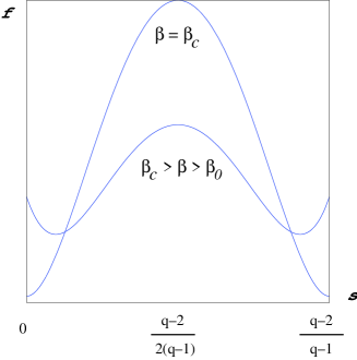
Figure 1: The free energy on $h_{T}$.

On $h_{T}$ the free energy has two minima $s_{-}$ and $s_{+}$ for which $f(s_{-})=f(s_{+})$. They satisfy the mean field equation (2) and thus are given by the parametric equations

$$(\beta,h)=(\beta_{s_{\pm}},-\frac{q-2}{2(q-1)}\beta_{s_{\pm}}+\ln(q-1))$$ (21)

where

$$\beta_{s}=\left(s-\frac{q-2}{2(q-1)}\right)^{-1}\ln\frac{1+(q-1)s}{(q-1)(1-s)}$$ (22)

and $s_{-}\in[0,\frac{q-2}{2(q-1)}]$, $s_{+}\in[\frac{q-2}{2(q-1)},\frac{q-2}{(q-1)}]$.

For $\beta_{0}<\beta\leqslant\beta_{c}^{(q)}$ (or equivalently $0\leqslant h<h_{0}$) these two minima are distinct: $s_{-}<s_{+}$. At ($\beta_{0},h_{0}$), $s_{-}=s_{+}=\frac{q-2}{2(q-1)}$, and at ($\beta_{c}^{(q)},0$), $s_{-}=0$ and $s_{+}=\frac{q-2}{q-1}$.

Outside of the segment (19), there is only one minimum $s_{0}$. This minimum is an analytic function of $\beta\operatorname{and}$ $h$, and $s_{0}\rightarrow s_{-}$ as $h\uparrow h_{T}$, $s_{0}\rightarrow s_{+}$ as $h\downarrow h_{T}$. In addition, on $h_{T}$, as $\beta$ increases from $\beta_{0}$ to $\beta_{c}^{(q)}$ (or equivalently as $h$ decreases from $h_{0}$ to $0$), $\beta x_{1}(s_{-})$ strictly decreases from $\beta_{0}/2>1$ to $\beta_{c}^{(q)}/q<1$, while $\beta x_{1}(s_{+})$ strictly increases from $\beta_{0}/2$ to $\beta_{c}^{(q)}(q-1)/q$. See below.

We now turn to the topological behavior.

Let ($\beta_{\operatorname{cp}},h_{\operatorname{cp}}$) the point of $h_{T}$ for which $\beta x_{1}(s_{-})=1$. This point is distinct from the two endpoints (20). It is given by the solution of the equation $(\beta_{\operatorname{cp}}-2)q=2(q-1)\ln(\beta_{\operatorname{cp}}-1)$ which can be solved by using the Lambert W function.

As a consequence of the above remarks, one gets the following topological behaviour for the system. On the thermodynamic line $h_{T}$:

1. at ($\beta_{\operatorname{cp}},h_{\operatorname{cp}}$), the largest component of $\mu_{\operatorname{CRC}}$ is either of order $n^{2/3}$ or of order $\Theta_{x_{1}(s_{+})}n$.

2. if $h_{\operatorname{cp}}<h\leqslant h_{0}$, the largest component of $\mu_{\operatorname{CRC}}$ is either of order $\Theta_{x_{1}(s_{-})}n$ or of order $\Theta_{x_{1}(s_{+})}n$.

3. if $0\leqslant h<h_{\operatorname{cp}}$, the largest component of $\mu_{\operatorname{CRC}}$ is either of order $\ln n$ or of order $\Theta_{x_{1}(s_{+})}n$.

The item 3 extends to the values $0\leqslant h<h_{\operatorname{cp}}$ what happens in item d) of the random cluster model for vanishing field. It implies that the thermodynamic and topological lines coincide there. This holds also at ($\beta_{\operatorname{cp}},h_{\operatorname{cp}}$), with a new behaviour in the sense that the giant component is of order $n^{2/3}$ or of order $\Theta_{x_{1}(s_{+})}n$.

The Kertész line is given in this range of temperature (and field) by

$$h_{K}^{(q)}(\beta)=h_{T}(\beta)\hskip 8.00003pt\operatorname{for}\hskip 8.00003pt\beta_{\operatorname{cp}}\leqslant\beta\leqslant\beta_{c}^{(q)}\hskip 8.00003pt\operatorname{or}\hskip 8.00003pt0\leqslant h\leqslant h_{\operatorname{cp}}$$ (23)

The item 2 shows that the giant component exhibits a jump, however, for given $h>h_{\operatorname{cp}}$, this giant component already appeared for lower values of $\beta$. The topological transition line is determined, as in case $q=2$, by eliminating $s$ between the mean field equation and the condition (17). This gives

$$h^{(q)}_{K}(\beta)=\frac{\beta-q}{q-1}-\ln\frac{\beta-1}{q-1}{\hskip 8.00003pt}\operatorname{for}{\hskip 8.00003pt}\beta\leqslant\beta_{\operatorname{cp}}\hskip 8.00003pt\operatorname{or}\hskip 8.00003pth\geqslant h_{\operatorname{cp}}$$ (24)

see Fig. 2. Below the Kertész line $h^{(q)}_{K}$ the largest component is of order $\ln n$, while above $h^{(q)}_{K}$ and outside of the segment (19), the largest component is of order $\Theta_{x_{1}(s_{0})}n$.

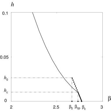
Figure 2: The thermodynamic transition curve: thick (solid, dashed) line; the topological transition curve: solid (thick, thin) line.

The symmetry of the free energy is better seen if we parametrize the magnetization $s$ by $z\in(\pm 1)$ as follows:

$$s=\frac{q-2}{2(q-1)}+\frac{q}{2(q-1)}z.$$ (25)

The corresponding densities are given by $x_{1}=\frac{1+z}{2}$, $x_{2}=\cdots=x_{q}=\frac{1-z}{2(q-1)}$, and the free energy decomposes immediately into its even and odd parts:

$$f(z) = \frac{1}{2}[(1+z)\ln(1+z)+(1-z)\ln(1-z)$$ (26)

$$-\beta\frac{q(1+z^{2})}{4(q-1)}-h-\ln\left(4(q-1)\right)]$$

$$+\frac{z}{2}\left[\ln(q-1)-\beta\frac{q-2}{2(q-1)}-h\right].$$

The first derivative of $f$ yields the mean field equation (2) while the second derivative is

$$f^{\prime\prime}(z)=\frac{1}{1-z^{2}}-\frac{\beta q}{4\left(q-1\right)}.$$ (27)

Thus f is convex when $\beta\leqslant\beta_{0}$ and has exactly one minima. When $\beta>\beta_{0}$ it has at most two local minimas. The analyticity of $s_{0}$ outside of $h_{T}$ is a consequence of $f^{\prime\prime}(z_{0})>0$. The monotonicity of $\beta x_{1}(s_{+})$ is trivial, that of $\beta x_{1}(s_{-})$ can be infered from the computation of the contour lines for $\beta x_{1}(s)$ below $h_{T}$.

4 Conclusion

To summarize, we have given the equation of the Kertész line of the mean–field Potts model and shown that when $q\geqslant 3$ this line exhibits a cusp at some $(\beta_{\operatorname{cp}},h_{\operatorname{cp}})$. For low fields ($h\leqslant h_{\operatorname{cp}})$ the Kertész line coincides with the thermodynamic transition line, and for large fields ($h\geqslant h_{0})$ only the topological transition remains while the thermodynamic transition disappears. In addition, at intermediate fields ($h_{\operatorname{cp}}<h<h_{0})$ the Kertész line separates from the thermodynamic line. This means that decreasing the temperature one sees first the appeareance of a giant component (on $h_{K}$) and, then on $h_{T}$, this component exhibits a jump. This behavior is new compared to what happens for the model on the $2$–dimensional regular lattice. There, no intermediate regime appears [4]. We expect for sufficiently high lattice dimensions, a behaviour similar to the model on the complete graph.

4.1 Acknowledgments

Warm hospitality and Financial support from the BiBoS Research Center, University of Bielefeld and Centre de Physique Théorique, CNRS Marseille are gratefully acknowledged.

References

- [1] J. Kertész, Physica A, 161:58, 1989.
- [2] A. Coniglio and W. Klein, J. Phys. A: Math. Gen., 13:2775, 1980.
- [3] C. M. Fortuin and P. W. Kasteleyn, Physica, 57:536, 1972.
- [4] Ph. Blanchard, D. Gandolfo, L. Laanait, J. Ruiz, and H. Satz, J. Phys. A: Math. Gen. , 41 (2008) 085001.
- [5] F. Y. Wu., Rev. Mod. Phys., 54:235–268, 1982.
- [6] M. Costeniuc, R. Ellis, and H. Touchette, J. Math. Phys., 46:063301, 2005.
- [7] M. Biskup, L. Chayes, and N. Crawford, J. Stat. Phys., 128:1139, 2006.
- [8] R.G. Edwards and A.D. Sokal, Phys. Rev. D, 38:2009–2012, 1988.
- [9] P. Erdös and A. Rényi, Publ. Math. Debrecen, 5:290–297, 1959.
- [10] B. Bollobás. Random Graphs. Academic Press, London, 1985.
- [11] S. Janson, T. Luczak, and A. Ruciński. Random Graphs. John Wiley & sons, New–York, 2000.
- [12] M. Biskup, L. Chayes, and S. Starr, Random Struct. & Algorithms, 31:354–370, 2007.
- [13] B. Bollobás, G. Grimmett, and S. Janson, Probab. Theor. Relat. Fields, 104:283, 1996.
- [14] G. Grimmett. The Random–Cluster Model. Springer–Verlag, Berlin, 2006.
- [15] M. Luczak and T. Luczak, Random Struct. & Algorithms, 28:215–246, 2005.