Shannon Information Capacity of Discrete Synapses

Abstract

There is evidence that biological synapses have only a fixed number of discrete weight states. Memory storage with such synapses behaves quite differently from synapses with unbounded, continuous weights as old memories are automatically overwritten by new memories. We calculate the storage capacity of discrete, bounded synapses in terms of Shannon information. For optimal learning rules, we investigate how information storage depends on the number of synapses, the number of synaptic states and the coding sparseness.

Memory in biological neural systems is believed to be stored in the synaptic weights. Various computational models of such memory systems have been constructed in order to study their properties and to explore potential hardware implementations. Storage capacity, and optimal learning rules have been studied both for single-layer associative networks (Willshaw et al., 1969; Dayan and Willshaw, 1991), studied here, and for auto-associative networks (Hopfield, 1982; Meunier and Nadal, 1995). Commonly, a synaptic weight in such models is represented by an unbounded continuous real number. However, more realistically, synaptic weights have values between some biophysical bounds. Furthermore, synapses might be restricted to occupy a limited number of synaptic states. Consistent with this, some experiments show that, physiologically, synaptic weight changes occur in steps (Petersen et al., 1998; O’Connor et al., 2005). In contrast to networks with continuous, unbounded synapses, in networks with discrete, bounded synapses old memories are overwritten by new ones, in other words, the memory trace decays (Nadal et al., 1986; Parisi, 1986; Amit and Fusi, 1994).

It is common to use the signal-to-noise ratio (SNR) to quantify memory storage (Fusi and Abbott, 2007; Dayan and Willshaw, 1991). When weights are unbounded, each stored pattern has the same SNR, and storage can simply be defined as the maximum number of patterns for which the SNR is larger than some fixed, minimum value. For discrete, bounded synapses performance must be characterized by two quantities: the initial SNR, and its decay rate. Altering the learning rules typically results in either 1) a decrease in initial SNR but a slower decay of the SNR (i.e. an increase in memory lifetime) (Fusi and Abbott, 2007), or 2) an increase in initial SNR but a decrease in memory lifetime. Optimization of the learning rule is ambivalent because an arbitrary trade-off must be made between these two effects.

The conflict between optimizing learning and optimizing forgetting can be resolved by analyzing the capacity of synapses in terms of Shannon information. Here we describe a framework for calculating the information capacity of bounded, discrete synapses, and use it to find optimal learning rules. We model a single neuron, and investigate how the information capacity depends on the number of synapses and the number of synaptic states, both for dense and sparse coding.

We consider a single neuron which has $n$ inputs. At each time step it stores a $n$-dimensional binary pattern with independent entries $x^{a}$, $a=1\ldots n$. The sparsity $p$ corresponds to the fraction of entries in $x$ that cause strengthening of the synapse. It is optimal to set the low state equal to $-p$, and the high state to $q=:(1-p)$, so that the probability density for inputs is given by $P(x)=q\delta(x+p)+p\delta(x-q)$ and $\langle x\rangle=0$. The case $p=\frac{1}{2}$ we term dense, furthermore, we assume that $p\leq\frac{1}{2}$, as the case $p\geq\frac{1}{2}$ is fully analogous. Although biological coding is believed to be sparse, we briefly note that in biology the relation between $p$ and coding sparseness is likely very complicated.

Each synapse occupies one of $W$ states. The corresponding values of the weight are assumed to be equidistantly spaced around zero and are written as a $W-$dimensional vector, i.e. for a 3-state synapse $\boldsymbol{w}=\{-1,0,1\}$, while for a 4-state synapse $\boldsymbol{w}=\{-2,-1,1,2\}$. In numerical analysis we have sometimes seen an increase in information by varying the values of the weight states, however this increase was always small. Note, that $\boldsymbol{w}$ is very different from the definition of a “weight vector” commonly used in network models.

The learning paradigm we consider is the following: during the learning phase a pattern is presented each time step, and the synapses are updated in an unsupervised manner. The learning algorithm is on-line, i.e. the synapses can only be updated when the pattern is presented. As bounded, discrete synapses store new memories at the expense of overwriting old ones, we can assume that sufficient patterns are stored such that the earliest pattern has almost completely decayed and the distribution of the synaptic weights has reached an equilibrium.

After learning, the neuron is tested on learned and novel patterns. Presentation of a learned pattern will yield an output which is on average larger than that for a novel pattern. The presentation of a novel, random pattern $\{x_{u}^{a}\}$ leads to a signal $h_{u}=\sum_{a}x_{u}^{a}\omega_{a}$, where the weights are $\omega_{a}$, $a=1,\ldots,n$. As this novel pattern will be uncorrelated to the weight, it has mean $\left\langle h_{u}\right\rangle=n\left\langle x\right\rangle\left\langle w\right\rangle=0$, and variance

$$\left\langle\Delta h_{u}^{2}\right\rangle=n\left[\left\langle x^{2}w^{2}\right\rangle-\left\langle x\right\rangle^{2}\left\langle w\right\rangle^{2}\right]=npq\left\langle w^{2}\right\rangle\,,$$ (1)

where $\left\langle w\right\rangle=\boldsymbol{w}.\boldsymbol{\pi}^{\infty}$, $\left\langle w^{2}\right\rangle=\sum_{i=1}^{W}w_{i}^{2}\pi{}_{i}^{\infty}$, and $\mathbf{\boldsymbol{\pi}^{\infty}}$ is the equilibrium distribution of weights.

Because the synapses are independent, and the performance is characterized statistically, we can use Markov transition matrices to define the learning (Fusi, 2002; Fusi and Abbott, 2007). If in the learning phase an input is high (low), the synapse is updated according to the matrix $M^{+}$ ($M^{-}$). Thus, the distribution of potentiated weights immediately after a high input is $\boldsymbol{\pi}^{+}(t=0)=M^{+}\boldsymbol{\pi}^{\infty}$. As subsequent, uncorrelated, patterns are learned, this signal decays according to $\boldsymbol{\pi}^{+}(t)=M^{t}\boldsymbol{\pi}^{+}(t=0)$, where $M=:pM^{+}+qM^{-}$ is the expected update matrix at each time-step. The equilibrium distribution $\boldsymbol{\pi}^{\infty}$ is identical to the eigenvector of $M$ with eigenvalue one. The mean signal for learned patterns is

$$\left\langle h_{\ell}\right\rangle(t)=npq\boldsymbol{w}^{T}M^{t}(M^{+}-M^{-})\boldsymbol{\pi}^{\infty}\,.$$ (2)

This signal decays such that the synapses contain most information on more recent patterns. The decay is typically exponential, with a time constant equal to the sub-dominant eigenvalue of $M$.

When tested with an equal mix of learned and unlearned patterns, the mutual information in the neuron’s output about whether a single pattern is learned or not is

$$I = \sum_{h,s=\{u,l\}}P(s)P(h|s)\log_{2}\frac{P(h|s)}{P(h)}$$

$$= \tfrac{1}{2}\sum_{h}P_{\ell}(h)\log_{2}\tfrac{2P_{\ell}(h)}{P_{\ell}(h)+P_{u}(h)}+P_{u}(h)\log_{2}\tfrac{2P_{u}(h)}{P_{\ell}(h)+P_{u}(h)}$$

where $P_{\ell}$ ($P_{u}$) denotes the distribution of the output of the neuron to learned (unlearned) patterns. If the two output distributions are perfectly separated, the learned pattern contributes one bit of information, whilst total overlap implies zero information storage. As the patterns are independent, the total information is the sum of the information over all patterns presented during learning.

Unfortunately, the full distributions of $h$ are complicated multinomials. Furthermore, it would be challenging for a biological readout to distinguish between two aribitrary distributions. Instead we impose a threshold between two possible responses, which could, say, correspond to the neuron firing or not. If the number of synapses is large, we can approximate the distribution of $h$ with a Gaussian and the information reduces to a function of the SNR

$$I(t)=1+r(t)\log_{2}r(t)+[1-r(t)]\log_{2}[1-r(t)]\,,$$ (4)

where $r(t)=\frac{1}{2}\mathrm{erfc}(\sqrt{\mathrm{SNR(t)}/8})$, and the SNR is defined as

$$\mathrm{SNR}(t)=\frac{{2\left(\left\langle h_{\ell}\right\rangle(t)-\left\langle h_{u}\right\rangle\right)}^{2}}{\left\langle\Delta h_{\ell}^{2}\right\rangle(t)+\left\langle\Delta h_{u}^{2}\right\rangle}\,.$$ (5)

In the numerical simulations we use Eqs. (4) and (5), but for the analytical expressions we assume the same variance of the output for learned and unlearned patterns, $\left\langle\Delta h_{\ell}^{2}\right\rangle(t)\approx\left\langle\Delta h_{u}^{2}\right\rangle$. Importantly, the information (4) is a saturating function of the SNR, and for very high SNR, the information is approximately one bit. Meanwhile for small SNR, the information is linear in the SNR, $I\approx\mathrm{SNR}/(4\pi\ln 2)$.

The total information per synapse is obtained by summing together the information of all patterns and dividing by the number of synapses, thus $I_{\mathrm{S}}=:{\frac{1}{n}\sum}_{t=0}^{\infty}I[\mathrm{SNR}(t)]$. In cases in which the initial SNR is very low

$$I_{\mathrm{S}}\approx\frac{1}{4\pi n\ln 2}\sum_{t=0}^{\infty}\mathrm{SNR}(t)\,.$$ (6)

In the opposite limit, when the initial SNR is very high, recent patterns contribute one bit. We approximate as if all patterns with more than 1/2 bit actually contribute one bit, whilst all patterns with less information contribute nothing. In this limit the information thus equals the number of patterns with more than 1/2 bit of information

$$I_{\mathrm{S}}=\frac{t_{c}}{n}\,,$$ (7)

where $t_{c}$ is implicitly defined as $I(t_{c})=1/2$.

The storage capacity depends on the $W\times W$ learning matrices $M^{+}$ and $M^{-}$. To find the maximal storage capacity we need to optimize these matrices, and this optimization will in general depend on the sparseness, the number of synapses, and the number of states per synapse. Because these are Markov transition matrices, their columns need sum to one, leaving $W(W-1)$ free variables per matrix. For dense patterns ($p=1/2$) one can impose additional symmetry $(M^{+})_{ij}=(M^{-})_{W-i,W-j}$.

In the case of binary synapses we write

$$M^{+}=\left(\begin{array}[]{cc}1-f_{+}&0\\ f_{+}&1\end{array}\right),\;\;M^{-}=\left(\begin{array}[]{cc}1&f_{-}\\ 0&1-f_{-}\end{array}\right)\,.$$ (8)

We first consider the limit of few synapses, for which the initial SNR is low, and use (6) to compute the information. ( We keep $np>1$ and $n\gtrsim 10$ to ensure that there are sufficient distinct patterns to learn.) We find

$$I_{\mathrm{S}}=\frac{pq}{\pi\ln 2}\frac{f_{+}^{2}f_{-}^{2}}{(pf_{+}+qf_{-})^{3}}\frac{1}{2-pf_{+}-qf_{-}}\,.$$ (9)

The values for $f_{+}$ and $f_{-}$ that yield maximal information depend on the value of the density $p$. For $0.11<p<0.89$, one has $f_{+}=f_{-}=1$, which gives equilibrium weight distribution $\boldsymbol{\pi}^{\infty}=(q,p)^{T}$, and

$$I_{\mathrm{S}}=\frac{pq}{\pi\ln 2}\,.$$ (10)

In this case the synapse is modified at every time-step and only retains the most recently presented pattern; the information stored on one pattern drops to zero as soon as the next pattern is learned.

For sparser patterns $p<0.11$ a second solution to Eq. (9) is optimal, for which $f_{+}=1$, $f_{-}\approx 2p$. I.e. potentiation occurs for every high input, but given a low input, depression only occurs stochasticly with a probability $2p$. As a result, forgetting is not instantaneous and the SNR decays exponentially with time constant $\tau=1/(6p)$. The associated weight distribution $\boldsymbol{\pi}^{\infty}\approx(2/3,1/3)^{T}$, which is interesting to compare to experiments in which about 80% of the synapses were found to be in the low state (O’Connor et al., 2005). The information per synapse is

$$I_{\mathrm{S}}=\frac{1}{\pi\ln 2}(\frac{2}{27}+\frac{p}{9})\,.$$ (11)

There are two important observations to be made from Eqs. (10-11): 1) the information remains finite at low $p$, 2) as long as the approximation is valid, each additional synapse contributes to the information.

We next consider the limit of many synapses, for which the initial SNR is high. With Eq. (7) we find

$$I_{\mathrm{S}}=\frac{1}{2\ln\left[1-f_{+}p-f_{-}q\right]}\ln\left[\frac{s}{4npq}\frac{(f_{+}p+f_{-}q)^{2}}{f_{+}^{2}f_{-}^{2}}\right]$$ (12)

where $s\approx 6.02$ is defined as the value of the SNR which corresponds to 1/2 bit of information. The optimal learning parameters are in this limit $f_{+}=e\sqrt{sq/pn}$ and $f_{-}=e\sqrt{sp/qn}$, leading to an equilibrium weight distribution $\boldsymbol{\pi}^{\infty}=(1/2,1/2)^{T}.$ In this regime the learning is stochastic, with the probability for potentiation/depression decreasing as the number of synapses increases. The corresponding information is

$$I_{\mathrm{S}}=\frac{1}{2e\sqrt{spqn}}\approx\frac{0.075}{\sqrt{pqn}}\,.$$ (13)

Hence, as $n$ becomes large, adding extra synapses no longer leads to substantial improvement in the information storage capacity. The memory decay time constant is $\tau=\sqrt{n}/(4e\sqrt{spq})$.

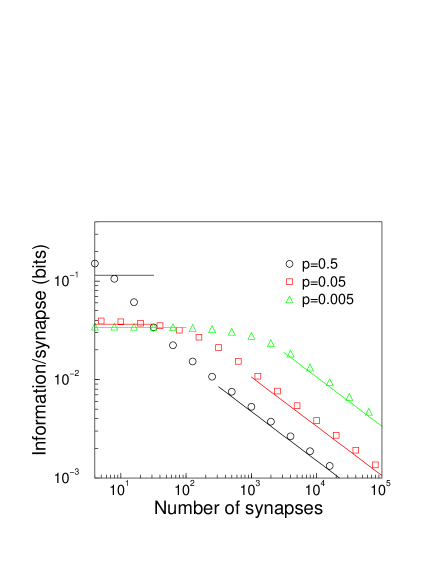
Figure 1: Information capacity of binary synapses. Information storage capacity per synapse versus the number of synaptic inputs, for dense (p=0.5), sparse (p=0.05) and very sparse (p=0.005) coding. Lines show analytic results, whilst points show numerical results. For small number of synapses, each additional synapse contributes to the information. However, for many synapses, the information per synapse decreases as $1/\sqrt{n}$.

To verify the above results, we carried out a numerical optimization of learning matrices. We find there is a smooth interpolation between the two limiting cases, and for a given sparseness there is a critical number of synapses beyond which the addition of further synaptic inputs does not substantially improve information storage capacity. This occurs when the initial SNR becomes of order 1. For dense patterns, this occurs for just a few synapses, whilst for sparse patterns this number is proportional to $p^{-1}$, see Fig. 1.

It is interesting to compare the storage capacity found here with that of a Willshaw net (Willshaw et al., 1969), which also involves binary synapses. In the Willshaw model, prior to learning, all synapses occupy the low state, whilst the learning process consists solely of potentiation of certain synapses. This means that as more patterns are presented, more synapses move to the up state, and eventually all memories are lost. However, when only a finite, optimal number of patterns are presented, such synapses perform well. When the task is to successfully reproduce an output pattern associated with each input pattern, the maximum capacity is 0.69 bits/synapse (Willshaw et al., 1969; Brunel, 1994). When measured for a binary response, as in the framework of this paper, this value is reduced. In the limit of few synapses, and sparse patterns, the storage capacity is approximately 0.11 bits/synapse, which is several times higher than the storage we obtain here. However, as the number of synapses increases, the storage capacity becomes proportional to $n^{-1}$, a faster decay than the $n^{-1/2}$ we find for our case.

Next, we examine whether storage capacity increases as the number of synaptic states increases. Even under small or large $n$ approximations, the information is in general a complicated function of the learning parameters, due to the complexity of the invariant eigenvector $\boldsymbol{\pi}^{\infty}$ of the general Markov matrix $M$. Thus, the optimal learning must be found numerically by explicitly varying all matrix elements. For large $n$ we find that the optimal transfer matrix is band diagonal, with the only transitions allowed being one-step potentiation or depression. Moreover, we find that for a fixed number of synaptic states, the (optimized) information storage capacity behaves similarly to that for binary synapses. In the dense ($p=1/2)$ case, in the limit of many synapses, the optimal learning rule takes the simple form

$$M=\frac{1}{2}\left(\begin{array}[]{ccccccc}2-f&1&0\\ f&0&1\\ 0&1&0\\ 0&0&1\\ &&&\ddots\\ &&&&0&1&0\\ &&&&1&0&f\\ &&&&0&1&2-f\end{array}\right)\,,$$ (14)

with $f=e\sqrt{s/n}$ . The equilibrium weight distribution is, somewhat surprisingly, peaked at both ends, and is low and flat in the middle, $\boldsymbol{\pi}^{\infty}\propto(1,f,f,\ldots,f,1)^{T}$. The information is

$$I_{\mathrm{S}}=\frac{W-1}{2fn}\ln\frac{f^{2}n}{s}=\frac{W-1}{e\sqrt{sn}}\,,$$ (15)

and the corresponding time constant for the SNR is given by $\tau=(W-1)\sqrt{n/s}/(2e)$. Validity of these results requires $fW$ to be small, to enable series expansion in $f$. Hence, we find that information grows linearly with the number of synaptic states, provided $W/\sqrt{n}\ll 1/(e\sqrt{s})$.

There appears to be no simple optimal transfer matrix in the sparse case, even in the large $n$ limit. However, a formula for the storage capacity which fits well with numerical results and is consistent with equations (13) and (15) is

$$I_{\mathrm{S}}=\frac{W-1}{2e\sqrt{spqn}}\,.$$ (16)

Assuming that this formula, as for the binary synapse, is the leading term in a series expansion in the two parameters $f_{+}=e\sqrt{sq/pn}$ and $f_{-}=e\sqrt{sp/qn},$ and that we need $Wf_{+}$ and $Wf_{-}$ small for it to be accurate, then its validity condition is $W\sqrt{q/np}\ll 1/(e\sqrt{s})$.

Numerical results agree with the equations above, and are illustrated together with the analytic results in Fig. 2. Thus, for fixed number of synapses, storage initially grows linearly with $W$. However, as $W$ becomes larger, capacity saturates and becomes independent of $W$. This behavior is consistent with that of a number of different (sub-optimal) learning rules studied in Ref. (Fusi and Abbott, 2007). These learning rules had the property that the product of the initial SNR and the time-constant $\tau$ of SNR decay is independent of $W$ (see Table 1 in (Fusi and Abbott, 2007) for this remarkable identity, noting that the SNR there equals its square root here). For large $W$, or equivalently small $n$, the initial SNR is small, and hence the information $I\sim\sum_{t}\mathrm{SNR(0)}\exp(-t/\tau)\sim\mathrm{SNR}(0)\tau$ is independent of $W$, as observed here, Fig. 2.

It is interesting to note that even unbounded synapses store only a limited amount of information. In the framework of this paper, the optimal local learning rule for unbounded synapses (optimized as in (Dayan and Willshaw, 1991)) yields $\mathrm{SNR}=n/m$, where $m$ is the number of patterns. This corresponds to storing 0.11 bits/synapse in the case that $m\gg n\gg 1$.

Figure 2: Information capacity of multi-state synapses. Information storage capacity per synapse versus the number $W$of synaptic states, for dense ($p=0.5$) and sparse ($p=0.05$) coding. Lines show analytic results (when available), whilst points show numerical results. For small number of synaptic states, storage capacity is increasing, but for larger numbers saturates.

Finally we study, in the large $n$ limit, the performance of a simple “hard-bound” learning rule, i.e. a learning rule with uniform equilibrium weight distribution. Under this rule, whose SNR dynamics were previously studied in Ref. (Fusi and Abbott, 2007), a positive (negative) input gives one step potentiation (depression) with probability $f_{+}$ ($f_{-}$). For $W\geq 4$ the optimal probabilities satisfy $f_{{}_{+}}p=f_{-}q\approx e\sqrt{s}W\sqrt{(W+1)/(W-1)}/(2\sqrt{3n})$ and the information storage capacity is

$$I_{\mathrm{S}}\approx\sqrt{\tfrac{3(W-1)}{spqn(W+1)}}\frac{1}{eW}\left[1-\cos(\tfrac{\pi}{W-1})\right]^{-1}\!\!\approx 0.053\times\frac{W}{\sqrt{pqn}}\,.$$ (17)

Here the latter approximation is for large $W.$ This sub-optimal learning rule gives an information capacity of the same functional form as the optimal learning rule, but performs only 70% as well.

Given that simple stochastic learning performs almost as well as the optimal learning rule, one may wonder how well a simple deterministic learning rule performs in comparison. For certain potentiation and depression, $f_{+}=f_{-}=1$ , one finds

$$I_{\mathrm{S}}=\frac{W^{2}}{\pi^{2}n}\ln\left(\frac{12n}{W^{2}s}\right)\,.$$ (18)

Although this grows faster with $W$, the $1/n$ behavior means this performs much worse than optimal stochastic learning rules. The memory decay time is in this case $\tau=W^{2}/\pi^{2}.$

In summary, learning using bounded, discrete weights can be analyzed using the Shannon information. There are two regimes: 1) when the number of synapses is small, the information per synapse is constant and approximately independent of the number of synaptic states, 2) when the number of synapses is large, the capacity per synapse decreases as $1/\sqrt{n}$. Furthermore, we find that in the second regime, the optimal transition matrices are band diagonal. In particular, in the dense case ($p=1/2$), the matrix Eq. (14) is optimal. The critical $n$ that separates these regimes is dependent on the sparseness and the number of weight states. Although there are currently no good biological estimates for either the number of weight states, or the sparsity, these results might indicate that the number of synapses is limited to prevent sub-optimal storage. When increasing the number of synaptic states, we find that for small numbers the information grows linearly, while for larger numbers it levels off and reaches a saturation point.