Instability of Hopf vector fields on Lorentzian Berger spheres

Abstract

In this work, we study the stability of Hopf vector fields on Lorentzian Berger spheres as critical points of the energy, the volume and the generalized energy. In order to do so, we construct a family of vector fields using the simultaneous eigenfunctions of the Laplacian and of the vertical Laplacian of the sphere. The Hessians of the functionals are negative when they act on these particular vector fields and then Hopf vector fields are unstable. Moreover, we use this technique to study some of the open problems in the Riemannian case.

2000 MSC: 58E15, 53C25, 58E20.

Key words and phrases: Energy and volume functionals, generalized energy, Hopf vector fields, Berger spheres.

1 Introduction

A smooth vector field $V$ on a Riemannian manifold $(M,g)$ can be seen as a map into its tangent bundle endowed with the Sasaki metric, $g^{S}$, defined by $g$. The volume of $V$ is the volume of $V(M)$ considered as a submanifold of $(TM,g^{S})$ . Analogously, we can define the energy of $V$ as the energy of the map $V:(M,g)\longrightarrow(TM,g^{S})$ and if $\tilde{g}$ is another metric on $M$, we define the generalized energy $E_{\tilde{g}}$ as the energy of $V:(M,\tilde{g})\to(TM,g^{S})$. These energies were introduced in [5] to study the relationship between the energy and the volume of vector fields. In particular, if we take either $\tilde{g}=g$ or $\tilde{g}=V^{*}g^{S}$, the generalized energy turns out to be, up to constant factors, the energy and the volume of the vector field respectively.

On a compact manifold $M$, the critical points of all these functionals should be parallel with respect to the Levi-Civita connection defined by $g$, so it is usual to restrict the functionals to the submanifold of unit vector fields. Obviously, if $M$ admits unit parallel vector fields, they are the absolute minimizers.

The geometrically simplest manifolds admitting unit vector fields but not parallel ones are odd-dimensional spheres. Hopf vector fields defined as those tangent to the fibres of the Hopf fibration $\pi:S^{2m+1}\longrightarrow\mathbb{C}P^{m}$ are very special unit vector fields. When both manifolds are endowed with their usual metrics, this map is a Riemannian submersion with totally geodesic fibres whose tangent space is generated by the unit vector field $V=JN$, where $N$ is the unit normal to the sphere and $J$ is the usual complex structure of $\mathbb{R}^{2m+2}$.

In [9], Gluck and Ziller showed that Hopf vector fields on the $3$-dimensional round spheres are the absolute minimizers of the volume and the analogous result for the energy was shown by Brito in [4]. For higher dimension, they are unstable critical points of the energy ([7], [16] and [17]).

All these results are independent of the radius of the sphere, but as concerns the stability as critical points of the volume, Borrelli and Gil-Medrano showed in [3] that for each $m>1$ there exists a critical value of the radius, such that, Hopf vector fields are stable critical points of the volume if and only if the radius is lower than or equal to this critical radius. By stable we mean that the Hessian of the functional is positive semi-definite.

In order to understand better these phenomena, in [6] Gil-Medrano and the author studied the behaviour of the Hopf vector field with respect to the volume and the energy when the metric considered on the sphere is the canonical variation of the Riemannian submersion given by the Hopf fibration. The metrics so constructed are known as Berger metrics, they consist in a $1$-parameter variation $g_{\mu}$ for $\mu\neq 0$. When $\mu>0$, the new metric is Riemannian and if $\mu<0$, the metric is Lorentzian and $V^{\mu}=1/\sqrt{-\mu}\,V$ is timelike. Moreover, they also studied the subset of $\mathbb{R}^{+}\times\mathbb{R}^{+}$ of pairs $(\mu,\lambda)$ such that the vector field $V^{\mu}$ is stable as a critical point of the generalized energy $E_{g_{\lambda}}$ on the spheres of dimension greater than three. The dimension three was studied in [11].

In Riemannian Berger spheres, the problem of determining the behaviour of Hopf vector fields is completely solved for the energy and the volume, but as concerns the generalized energy $E_{g_{\lambda}}$, there exist values of $\lambda$ and $\mu$ for which the stability of Hopf vector fields is still an open problem. For Lorentzian Berger spheres, the technique used to show stability in the Riemannian case does not allow us to conclude the stability in any case and only a partial result concerning the instability is shown in [6]. These instability results, as in the Riemannian case, have been obtained computing the Hessian in the direction of the vector fields $A_{a}=a-\langle a,V\rangle V-\langle a,N\rangle N$ for all $a\in\mathbb{R}^{2m+2}$, $a\neq 0$. These vector fields can be seen as the projection onto $V^{\bot}$ of the gradient of an eigenfunction associated to the first eigenvalue of the Laplacian of the sphere.

In this work, we construct new directions using the simultaneous eigenfunctions of the Laplacian and of the vertical Laplacian $\Delta_{v}(f)=-V(V(f))$ of the sphere. More precisely, we consider vector fields $C_{2s}={\rm grad}^{\mu}f_{2s}-\varepsilon_{\mu}V^{\mu}(f_{2s})f_{2s}$, where $f_{2s}$ is a polynomial of degree $2s$ in $\mathbb{R}^{2m+2}$ such that its restriction to the sphere is a simultaneous eigenfunction of the Laplacian and of the vertical Laplacian. Here $\varepsilon_{\mu}=\mu/|\mu|$. These vector fields verify that $\nabla^{\mu}_{V^{\mu}}C_{2s}=(\mu-2s)/\sqrt{|\mu|}\ JC_{2s}$ and they allow us to prove in Section $3$ that on Lorentzian Berger spheres, the Hopf vector fields $V^{\mu}$ are unstable critical points of the energy, the volume and the generalized energy $E_{g_{\lambda}}$ for all $\lambda<0$. The eigenfunctions of $\Delta_{v}$ have been also used to study, for example, the harmonic index and nullity of the Hopf map (see [12]).

In Section $4$, we use the ideas introduced in the previous section to complete the results in [11] and then we solve completely the problem of determining the stability of Hopf vector fields with respect to the generalized energy $E_{g_{\lambda}}$ in the Riemannian Berger $3$-sphere. In particular, we prove that if $\lambda>(\mu-3)^{2}/(\mu-2)$ and $\mu>2$, or if $\lambda>\mu-4$ and $\mu>4$, then $V^{\mu}$ is an unstable critical point of $E_{g_{\lambda}}$. Again, we need to consider vector fields more complicated that the vectors fields $A_{a}$. So, the simultaneous eigenfunctions of the Laplacian and of the vertical Laplacian play an important role in the resolution of these problems in the sphere. For spheres of upper dimension, we can use the vector fields $C_{2s}$ to improve the results in [6] concerning the generalized energy, but it is not sufficient to solve completely the problem.

2 Preliminaries

Given a Riemannian manifold $(M,g)$, the Sasaki metric $g^{S}$ on the tangent bundle $TM$ is defined, using $g$ and its Levi-Civita connection $\nabla$, as follows:

$$g^{S}(\zeta_{1},\zeta_{2})=g(\pi_{*}\circ\zeta_{1},\pi_{*}\circ\zeta_{2})+g(\kappa\circ\zeta_{1},\kappa\circ\zeta_{2}),$$

where $\pi:TM\to M$ is the projection and $\kappa$ is the connection map of $\nabla$. We will consider also its restriction to the tangent sphere bundle, obtaining the Riemannian manifold $(T^{1}M,g^{S}).$

As in [5], for each metric $\tilde{g}$ on $M$ we can define the generalized energy of the vector field $V$, denoted $E_{\tilde{g}}(V)$, as the energy of the map $V:(M,\tilde{g})\to(TM,g^{S})$ that is given by

$$E_{\tilde{g}}(V)=\frac{1}{2}\int_{M}\operatorname{tr}L_{(\tilde{g},V)}\,{\rm dv}_{\tilde{g}},$$

where $L_{(\tilde{g},V)}$ is the endomorphism determined by $V^{*}g^{S}(X,Y)=\tilde{g}(L_{(\tilde{g},V)}(X),Y)$. This energy can also be written as

$$E_{\tilde{g}}(V)=\frac{1}{2}\int_{M}\sqrt{\operatorname{det}P_{\tilde{g}}}\,\operatorname{tr}(P_{\tilde{g}}^{-1}\circ L_{V})\,{\rm dv}_{g},$$ (1)

where $P_{\tilde{g}}$ and $L_{V}$ are defined by $\tilde{g}(X,Y)=g(P_{\tilde{g}}(X),Y)$ and $V^{*}g^{S}(X,Y)=g(L_{V}(X),Y)$, respectively. By the definition of the Sasaki metric, $L_{V}=\operatorname{Id}+(\nabla V)^{t}\circ\nabla V$. In particular, for $\tilde{g}=g$

$$E_{g}(V)=\frac{1}{2}\int_{M}\operatorname{tr}L_{V}\,{\rm dv}_{g}=\frac{n}{2}vol(M,g)+\frac{1}{2}\int_{M}\|\nabla V\|^{2}\,{\rm dv}_{g}.$$ (2)

This functional is known as the energy and will be represented by $E$. Its relevant part, $B(V)=\frac{1}{2}\int_{M}\|\nabla V\|^{2}\,{\rm dv}_{g}$, is known as the total bending of $V$ and its restriction to unit vector fields has been widely studied by Wiegmink in [15], (see also [16]).

On the other hand, the volume of a vector field $V$ is defined as the $n$-dimensional volume of the submanifold $V(M)$ of $(TM,g^{S})$. It is given by

$$F(V)=\int_{M}\sqrt{\operatorname{det}L_{V}}\,{\rm dv}_{g}.$$ (3)

Since for $\tilde{g}=V^{*}g^{S}$ we have $P_{\tilde{g}}=L_{V}$, then (1) and (3) give

$$F(V)=\frac{2}{n}E_{V^{*}g^{S}}(V).$$

The first variation of the generalized energy has been computed in [5]. It has been also shown there that $V$ is a critical point of $F$ if and only if $V$ is a critical point of $E_{V^{*}g^{S}}$ and that, on a compact $M$, a critical vector field of any of these generalized energies should be parallel. So, it is usual to restrict these functionals to the submanifold of unit vector fields.

The following proposition shown in [5] generalizes the characterization of critical points of the total bending in [15] and of the volume in [7].

Proposition 2.1.

Let $(M,g)$ be a Riemannian manifold, a unit vector field $V$ is a critical point of $E_{\tilde{g}}$ if and only if

$$\omega_{(V,\tilde{g})}\,(V^{\bot})=\{0\},$$

with $\ \omega_{(V,\tilde{g})}=C_{1}^{1}\nabla K_{(V,\tilde{g})}\$ and $\ K_{(V,\tilde{g})}=\sqrt{\operatorname{det}P_{\tilde{g}}}\ P_{\tilde{g}}^{-1}\circ(\nabla V)^{t}.$

Remark 2.2.

For a $(1,1)$-tensor field $K$, if $\{E_{i}\}$ is a $g$-orthonormal local frame,

$$C_{1}^{1}\nabla K(X)=\sum_{i}g((\nabla_{E_{i}}K)X,E_{i}).$$

Moreover, in [8] it was proved that a unit vector field is a critical point of $F$ if and only if it defines a minimal immersion in $(T^{1}M,g^{S})$.

Theorem 2.3 ([7]).

Let $V$ be a unit vector field on the Riemannian manifold $(M,g)$.

a) If $V$ is a critical point of $E_{\tilde{g}}$, the Hessian of $E_{\tilde{g}}$ at $V$ acting on $A\in V^{\bot}$ is given by

$$(HessE_{\tilde{g}})_{V}(A)=\int_{M}\|A\|^{2}\omega_{(V,\tilde{g})}\,(V)\,{\rm dv}_{g}+\int_{M}\sqrt{\operatorname{det}P_{\tilde{g}}}\ \operatorname{tr}\Big{(}P_{\tilde{g}}^{-1}\circ(\nabla A)^{t}\circ\nabla A\Big{)}\,{\rm dv}_{g}.$$

b) If $V$ is a critical point of the energy, the Hessian of $E$ at $V$ acting on $A\in V^{\bot}$ is given by

$$(HessE)_{V}(A)=\int_{M}\|A\|^{2}\omega_{(V,g)}(V)\,{\rm dv}_{g}+\int_{M}\|\nabla A\|^{2}\,{\rm dv}_{g}.$$

c) Let $V$ be a unit vector field defining a minimal immersion, the Hessian of $F$ at $V$ acting on $A\in V^{\bot}$ is given by

$$(HessF)_{V}(A)\ = \!\!\int_{M}\|A\|^{2}\omega_{V}(V)\,{\rm dv}_{g}+\int_{M}\frac{2}{\sqrt{\operatorname{det}L_{V}}}\ \sigma_{2}(K_{V}\circ\nabla A)\,{\rm dv}_{g}$$

$$- \int_{M}\operatorname{tr}\Big{(}L_{V}^{-1}\circ(\nabla A)^{t}\circ\nabla V\circ K_{V}\circ\nabla A\Big{)}\,{\rm dv}_{g}$$

$$+ \int_{M}\sqrt{\operatorname{det}L_{V}}\ \operatorname{tr}\Big{(}L_{V}^{-1}\circ(\nabla A)^{t}\circ\nabla A\Big{)}\,{\rm dv}_{g},$$

where $\sigma_{2}$ is the second elementary symmetric polynomial function. In particular, $\sigma_{2}(K_{V}\circ\nabla A)=(\operatorname{tr}(K_{V}\circ\nabla A))^{2}-\operatorname{tr}(K_{V}\circ\nabla A)^{2}$.

The generalized energy can be defined for any $g$ and $\tilde{g}$ semi-Riemannian metrics on the manifold $M$. In particular, in a Lorentzian manifold, the energy is defined for all vector fields. Nevertheless, the volume of a reference frame (unit timelike vector field) $V$ is not always defined, since the $2$-covariant field $V^{*}g^{S}$ can be degenerated. Due to this, we study the volume restricted to unit timelike vector fields for which $V^{*}g^{S}$ is a Lorentzian metric on $M$. We will denote this set of vector fields by $\Gamma^{-}(T^{-1}M)$ and it is an open subset of the set of smooth references frames. If $V$ belongs to $\Gamma^{-}(T^{-1}M)$, then ${\rm det}\,L_{V}>0$ and the volume is well defined.

The condition for a reference frame to be a critical point of the generalized energy on a Lorentzian manifold is the same condition that the one given by Proposition 2.1 for Riemannian metrics. If we compute the second variation, we obtain the following

Proposition 2.4.

Let $V$ be a unit timelike vector field on a compact Lorentzian manifold $(M,g)$.

1. If $V$ is a critical point of the generalized energy $E_{\tilde{g}}$ and $A\in V^{\bot}$, then

   $$(HessE_{\tilde{g}})_{V}(X)=-\int_{M}\|X\|^{2}\omega_{(V,\tilde{g})}(V)\,{\rm dv}_{g}+\int_{M}{\rm tr}(L_{\tilde{g}}\circ(\nabla X)^{t}\circ\nabla X)\,{\rm dv}_{g}.$$ (4)

2. [10] If $V$ is a critical point of the energy, the Hessian of $E$ at $V$ acting on $A\in V^{\bot}$ is given by

   $$(HessE)_{V}(A)=-\int_{M}\|A\|^{2}\omega_{(V,g)}(V)\,{\rm dv}+\int_{M}\|\nabla A\|^{2}\,{\rm dv}.$$

3. [10] For a unit timelike vector field $V\in\Gamma^{-}(T^{-1}M)$ defining a minimal immersion, the Hessian of $F$ at $V$ acting on $A\in V^{\bot}$ is given by

   $$(HessF)_{V}(A)\ = - \int_{M}\|A\|^{2}\omega_{V}(V)\,{\rm dv}+\int_{M}\frac{2}{\sqrt{\operatorname{det}L_{V}}}\ \sigma_{2}(K_{V}\circ\nabla A)\,{\rm dv}$$

   $$- \int_{M}\operatorname{tr}\Big{(}L_{V}^{-1}\circ(\nabla A)^{t}\circ\nabla V\circ K_{V}\circ\nabla A\Big{)}\,{\rm dv}$$

   $$+ \int_{M}\sqrt{\operatorname{det}L_{V}}\ \operatorname{tr}\Big{(}L_{V}^{-1}\circ(\nabla A)^{t}\circ\nabla A\Big{)}\,{\rm dv}.$$

The expression of the Hessian of the generalized energy given by (4) is obtained by straightforward computation in a similar way that in the Riemannian case, so we have omitted the details.

Remark 2.5.

Let us point out that if we compare the above expressions of the Hessian with those obtained for Riemannian metrics, the only difference is the minus sign of the first term of the expression of the Hessian.

Hopf vector fields on odd-dimensional spheres are tangent to the fibres of the Hopf fibration $\pi:(S^{2m+1},g)\to(\mathbb{C}^{m},\overline{g})$, where $g$ is the usual metric of curvature $1$ and $\overline{g}$ is the Fubini-Study metric with sectional curvatures between $1$ and $4$. This map is a Riemannian submersion with totally geodesic fibres whose tangent space is generated by the unit vector field $V=JN$, where $N$ is the unit normal to the sphere and $J$ is the usual complex structure of $\mathbb{R}^{2m+2}$; in other words, $V(p)=ip$.

In $S^{2m+1}$ we can consider the canonical variation $g_{\mu}$, with $\mu\neq 0$, of the usual metric $g$,

$$g_{\mu}|_{V^{\bot}}=g|_{V^{\bot}},\qquad g_{\mu}(V,V)=\mu g(V,V),\qquad g_{\mu}(V,V^{\bot})=0.$$ (5)

When $\mu>0$ the new metric is Riemannian and if $\mu<0$ the metric is Lorentzian and $V$ is timelike.

For all $\mu\not=0$, the map $\pi:(S^{2m+1},g_{\mu})\to(\mathbb{C}^{m},\overline{g})$ is a semi-Riemannian submersion with totally geodesic fibres. $(S^{3},g_{\mu})$, with $\mu>0$, is known as a Berger sphere. We will use the same name for all dimension and we will call $V^{\mu}=\frac{1}{\sqrt{|\mu|}}V$ the Hopf vector field. It is a unit Killing vector field with geodesic flow.

We denote by $\bar{\nabla}$ the Levi-Civita connection on $\mathbb{R}^{2m+2}.$ The Levi-Civita connection $\nabla$ on $(S^{2m+1},g)$ is $\nabla_{X}Y=\bar{\nabla}_{X}Y-<\bar{\nabla}_{X}Y,N>N$ and $\bar{\nabla}_{X}V=J\bar{\nabla}_{X}N=JX.$ Therefore $\nabla_{V}V=0$ and if $<X,V>=0$ then $\nabla_{X}V=JX.$

Using Koszul formula, one obtains the relation of $\nabla^{\mu}$, the Levi-Civita connection of the metric $g_{\mu}$, with $\nabla$

$$\nabla^{\mu}_{V}X=\nabla_{V}X+(\mu-1)\nabla_{X}V,\qquad\nabla^{\mu}_{X}V=\mu\nabla_{X}V,\qquad\nabla^{\mu}_{X}Y=\nabla_{X}Y,$$ (6)

for all $X,Y$ in $V^{\bot}$.

It has been shown in [6] that,

Proposition 2.6.

For all $\mu,\lambda\not=0$, the map $V^{\mu}:(S^{2m+1},g_{\lambda})\to(T^{1}(S^{2m+1}),g_{\mu}^{S})$ is harmonic.

Since $(V^{\mu})^{*}g_{\mu}^{S}=(1+|\mu|)g_{\lambda}$ where $\lambda=\mu/(1+|\mu|)$, as a consequence of the Proposition above, we have the following

Corollary 2.7 ([6]).

For all $\mu\not=0$, the Hopf vector field $V^{\mu}$ is a critical point of the generalized energy $E_{g_{\lambda}}$, for all $\lambda\not=0$, and it defines a minimal immersion.

Remark 2.8.

When $\mu<0$, $V^{\mu}$ induces on the sphere a Lorentzian metric $(V^{\mu})^{*}g_{\mu}^{S}$ and the Hopf vector field is a critical point of the volume restricted to the set of unit timelike vector fields verifying this condition.

The second variation of the energy and the volume at Hopf vector fields on Berger spheres has been computed in [6]. The expression of the Hessian of the generalized energy $E_{g_{\lambda}}$ is also computed in [6] for Riemannian Berger spheres. In a similar way, by straightforward computation, we can obtain the second variation of the generalized energy $E_{g_{\lambda}}$ in the Lorentzian case.

Proposition 2.9.

Let $V^{\mu}$ be the Hopf unit vector field on $(S^{2m+1},g_{\mu})$. For each vector field $A$ orthogonal to $V^{\mu}$ we have

$$\textrm{a) }(HessE_{g_{\lambda}})_{V^{\mu}}(A)=\int_{S^{2m+1}}\Big{(}-2m\varepsilon_{\mu}\sqrt{|\lambda\mu|}\ \|A\|^{2}+\sqrt{|\lambda/\mu|}\ \|\nabla^{\mu}A\|^{2}$$

$$\hskip 115.63243pt+\ (\varepsilon_{\lambda}\sqrt{|\mu/\lambda|}-\varepsilon_{\mu}\sqrt{|\lambda/\mu|}\ )\ \|\nabla^{\mu}_{V^{\mu}}A\|^{2}\Big{)}\,{\rm dv}_{\mu}.$$

$$\textrm{b) }(HessE)_{V^{\mu}}(A)=\int_{S^{2m+1}}\Big{(}-2m\mu\|A\|^{2}+\|\nabla^{\mu}A\|^{2}\Big{)}\,{\rm dv}_{\mu}.$$

$$\textrm{c) }(HessF)_{V^{\mu}}(A)=(1+|\mu|)^{m-2}\int_{S^{2m+1}}\Big{(}\|\nabla^{\mu}A\|^{2}+\ \mu\|\nabla^{\mu}_{V^{\mu}}A+\varepsilon_{\mu}\sqrt{|\mu|}JA\|^{2}$$

$$\hskip 115.63243pt+\mu(-2m-2m|\mu|+2\varepsilon_{\mu}+2\varepsilon_{\mu}(m-\mu))\|A\|^{2}\Big{)}\,{\rm dv}_{\mu}.$$

Where $\varepsilon_{\mu}=\mu/|\mu|$ and $\varepsilon_{\lambda}=\lambda/|\lambda|$.

Finally, let us recall some results concerning the vertical Laplacian.

Let $\pi:(M,g)\longrightarrow(N,h)$ be a Riemannian submersion and let $\Delta$ the Laplacian of $(M,g)$.

Definition 2.10 ([1]).

The vertical Laplacian $\Delta_{v}$ of $(M,g)$ is the differential operator given by

$$(\Delta_{v}f)(x)=(\Delta_{F_{x}}(f_{|_{F_{x}}}))(x),$$

where $F_{x}=\pi^{-1}(\pi(x))$ is the fibre of $\pi$ passing through $x$ and $\Delta_{F_{x}}$ is the Laplacian of the induced metric by $M$ on $F_{x}$.

The difference operator $\Delta_{h}=\Delta-\Delta_{v}$ is called the horizontal Laplacian.

Bérard-Bergery and Bourguignon, showed in [1] that if $\pi$ is a Riemannian submersion with totally geodesic fibres, then $\Delta$ and $\Delta_{v}$ commute. So, when $M$ is compact and connected, $L^{2}(M)$ admits a Hilbert basis consisting of simultaneous eigenfunctions of both operators.

On $(S^{2m+1},g)$, it is known (see [2]) that the eigenvalues of the Laplacian are $\lambda_{k}=k(k+2m)$ with $k=0,1,2,\ldots$. Moreover, the eigenvalues of the vertical Laplacian $\Delta_{v}$ are $\phi_{l}=l^{2}$ with $l=0,1,2,\ldots$. Then, as can be seen in [1] and [13], using that the Laplacian of the metrics $g_{\mu}$ is, $\Delta^{\mu}=\mu^{-1}\,\Delta_{v}+\Delta_{h}$, the eigenvalues of $\nabla^{\mu}$ are of the type

$$\lambda^{\mu}_{k,l} = (\lambda_{k}-\phi_{l})+\frac{1}{\mu}\phi_{l}=k(k+2m)-l^{2}+\frac{1}{\mu}l^{2},\qquad k\geq l.$$ (7)

In the above expression not all values of $k$ and $l$ are possible.

Besides, Tanno showed that,

Lemma 2.11 ([14]).

On $S^{2m+1}$, for each eigenvalue $\lambda_{k}$ of $\Delta$, the space of eigenfunctions $\mathcal{P}^{k}$ admits an orthogonal decomposition

$$\mathcal{P}^{k}=\mathcal{P}^{k}_{k}+\mathcal{P}^{k}_{k-2}+\cdots+\mathcal{P}^{k}_{k-2[k/2]},$$

where $[k/2]$ is the integer part of $k/2$, and for $f\in\mathcal{P}^{k}_{k-2p}$

$$V(V(f))=-(k-2p)^{2}f,\qquad 0\leq p\leq[k/2].$$

Some of the $\mathcal{P}^{k}_{l}$ could be trivial.

Since $\Delta_{v}(f)=-V(V(f))$, the problem of determining which spaces $\mathcal{P}^{k}_{l}$ are not trivial is related to that of determining the permitted combinations of $k$ and $l$ in (7).

In the following sections, we will use that $\mathcal{P}^{k}_{k}\neq\{0\}$ for all $k$ (see [14]), that is to say, for all $k>0$, $\lambda^{\mu}_{k,k}=k(2m+\frac{1}{\mu}k)$, is an eigenvalue of $\Delta^{\mu}$.

3 Lorentzian Berger spheres

The instability results in Riemannian Berger spheres have been obtained by computing the Hessians when they act on the vector fields $A_{a}=a-\langle a,V\rangle V-\langle a,N\rangle N$ for all $a\in\mathbb{R}^{2m+2}$, $a\neq 0$. These vector fields can be seen as the projection onto $V^{\bot}$ of the gradient of an eigenfunction associated to the first eigenvalue of the Laplacian. For Lorentzian Berger spheres, if we compute the Hessians in the direction of these particular vector fields, we obtain

Lemma 3.1.

Let $V^{\mu}$ be the Hopf unit vector field on $(S^{2m+1},g_{\mu})$, with $\mu<0$. For each $a\in\mathbb{R}^{2m+2}$, $a\not=0$ we have:

$$\textrm{a) }(HessE)_{V^{\mu}}(A_{a})=\frac{\sqrt{-\mu}m}{m+1}|a|^{2}\Big{(}(1-2m)\mu+2+\frac{(\mu-1)^{2}}{\mu}\Big{)}{\rm vol}(S^{2m+1}).$$

$$\textrm{b) }(HessF)_{V^{\mu}}(A_{a})=(1-\mu)^{m-2}\frac{\sqrt{-\mu}m}{m+1}|a|^{2}f(m,\mu){\rm vol}(S^{2m+1}),$$

where $f(m,\mu)=\Big{(}(2m-1)\mu^{2}+(1-4m)\mu+2+(1-\mu)\frac{(\mu-1)^{2}}{\mu}\Big{)}.$

As a consequence,

Proposition 3.2 ([6]).

Let $V^{\mu}$ be the unit Hopf vector field on $(S^{2m+1},g_{\mu})$, with $\mu<0$.

• If $(2m-2)\mu^{2}<1$, then $V^{\mu}$ is unstable for the energy.

• If $(2-2m)\mu^{3}+(4m-4)\mu^{2}+\mu<1$, then $V^{\mu}$ is unstable for the volume.

In particular, on $(S^{3},g_{\mu})$ the Hopf vector field is unstable for the energy and the volume for all values of $\mu<0$.

The alternative expressions of the Hessians used to show stability in the Riemannian case (see [6]) can be extended to include negative values of $\mu$, but they do not allow us to conclude the stability of Hopf vector fields in any case. In fact, we are going to prove that they are always unstable. Moreover, we will study the behaviour of Hopf vector fields with respect to the generalized energy $E_{g_{\lambda}}$.

In order to do so, we are going to consider new directions obtained from functions that are simultaneous eigenfunctions of the Laplacian and of the vertical Laplacian of the sphere.

Let $f$ be a harmonic and homogeneous polynomial of degree $s$ in $\mathbb{R}^{2m+2}$, then the restriction of $f$ to the sphere, denoted also by $f$ for simplicity, is an eigenfunction associated to the eigenvalue $s\,(2m+s)$ of the Laplacian of the sphere with the usual metric. Moreover, we take $f$ verifying that

$$\overline{Hess}f(u,Jv)=\overline{Hess}f(Ju,v)$$ (8)

for all $u$, $v$ vector fields in $\mathbb{R}^{2m+2}$, where $\overline{Hess}$ represents the Hessian in $\mathbb{R}^{2m+2}$. In the sequel, we will denote with a bar the geometrical operators related to the Euclidean space $\mathbb{R}^{2m+2}$.

We will use condition (8) to assure that if $\{N,E_{i},V,JE_{i}\}$ is a $J$-orthonormal local frame in $\mathbb{R}^{2m+2}$ then

$$\overline{Hess}f(E_{i},E_{i})+\overline{Hess}f(JE_{i},JE_{i})=0,\quad\forall\ 1\leq i\leq m,$$

and

$$\overline{Hess}f(V,V)+\overline{Hess}f(N,N)=0.$$

Proposition 3.3.

Let $f$ be a harmonic and homogeneous polynomial of degree $s$ in $\mathbb{R}^{2m+2}$ satisfying (8), then

• If $\Delta^{\mu}$ denotes the Laplacian of Berger spheres and $\Delta^{\mu}_{v}$ the vertical Laplacian,

  $$\Delta^{\mu}f=(2ms+\frac{s^{2}}{\mu})f\quad\textrm{ and }\quad\Delta^{\mu}_{v}(f)=\frac{s^{2}}{\mu}f.$$

  In other words, $f\in\mathcal{P}^{s}_{s}$.

• If $C={\rm grad}^{\mu}f-\varepsilon_{\mu}V^{\mu}(f)V^{\mu}$, then $\nabla^{\mu}_{V^{\mu}}C=(\mu-s)/\sqrt{|\mu|}\ JC$.

Proof.

If $u,v\in(V^{\mu})^{\bot}$ then

$$(Hess)^{\mu}f(V^{\mu},u) = V^{\mu}(u(f))-(\nabla^{\mu}_{V^{\mu}}u)f=\overline{Hess}f(V^{\mu},u)+\frac{1-\mu}{\sqrt{|\mu|}}Ju(f),$$

$$(Hess)^{\mu}f(u,v) = u(v(f))-(\nabla^{\mu}_{u}v)f=\overline{Hess}f(u,v)-\langle u,v\rangle N(f),$$

$$(Hess)^{\mu}f(V^{\mu},V^{\mu}) = V^{\mu}(V^{\mu}(f))=\overline{Hess}f(V^{\mu},V^{\mu})-\frac{1}{|\mu|}N(f).$$

Moreover, using (8) and the fact that $N(f)=s\,f$, we have that

$$\overline{Hess}f(V^{\mu},V^{\mu})=-\frac{\overline{Hess}f(N,N)}{|\mu|}=\frac{N(f)-N(N(f))}{|\mu|}=\frac{s(1-s)}{|\mu|}f.$$

Then, since $f$ is a harmonic polynomial,

$$\Delta^{\mu}(f) = -{\rm tr}(Hess)^{\mu}f=-\sum_{i=1}^{2m}(Hess)^{\mu}f(E_{i},E_{i})-\varepsilon_{\mu}\,(Hess)^{\mu}f(V^{\mu},V^{\mu})$$

$$= -\sum_{i=1}^{2m}\overline{Hess}f(E_{i},E_{i})+2mN(f)+\frac{s^{2}}{\mu}f$$

$$= (2ms+\frac{s^{2}}{\mu})f,$$

and

$$\Delta^{\mu}_{v}(f)=-\varepsilon_{\mu}V^{\mu}(V^{\mu}(f))=-\varepsilon_{\mu}(\overline{Hess}f(V^{\mu},V^{\mu})-\frac{N(f)}{|\mu|})=\frac{s^{2}}{\mu}f.$$

To show b), since $\nabla^{\mu}C=g_{\mu}^{-1}(Hess)^{\mu}f-\varepsilon_{\mu}\,\nabla^{\mu}(V^{\mu}(f)V^{\mu})$,

$$g_{\mu}(\nabla^{\mu}_{V^{\mu}}C,E_{j}) = (Hess)^{\mu}f(V^{\mu},E_{j})-\varepsilon_{\mu}\,g_{\mu}(\nabla^{\mu}_{V^{\mu}}(V^{\mu}(f)V^{\mu}),E_{j})$$

$$= \overline{Hess}f(V^{\mu},E_{j})+\frac{1-\mu}{\sqrt{|\mu|}}\,JE_{j}(f)$$

$$= \frac{1}{\sqrt{|\mu|}}\,(\overline{Hess}f(N,JE_{j})+(1-\mu)JE_{j}(f))$$

$$= \frac{1}{\sqrt{|\mu|}}\,((s-1)\langle\overline{{\rm grad}}f,JE_{j}\rangle+(1-\mu)JE_{j}(f))$$

$$= \frac{s-\mu}{\sqrt{|\mu|}}\,JE_{j}(f)=\frac{\mu-s}{\sqrt{|\mu|}}\,g_{\mu}(JC,E_{j}),$$

and therefore $\nabla^{\mu}_{V^{\mu}}C=\frac{\mu-s}{\sqrt{|\mu|}}\,JC$. ∎

Proposition 3.4.

Let $V^{\mu}$ be the unit Hopf vector field in $(S^{2m+1},g_{\mu})$ with $\mu\neq 0$ and $C={\rm grad}^{\mu}f-\varepsilon_{\mu}V^{\mu}(f)V^{\mu}$, where $f$ is a harmonic and homogeneous polynomial of degree $s$ verifying (8), then:

$$\textrm{a) }(HessE_{g_{\lambda}})_{V^{\mu}}(C)=\sqrt{\frac{|\lambda|}{|\mu|}}\int_{S^{2m+1}}\Big{(}\big{(}2ms((1-2m)\mu+\frac{(s-\mu)^{2}}{\lambda}-4(s-1)^{2}$$

$$\hskip 180.67499pt+2s)-4s^{2}(s-1)^{2})\big{)}f^{2}+\|\overline{Hess}f\|^{2}\Big{)}\,{\rm dv}_{\mu},$$

$$\textrm{b) }(HessE)_{V^{\mu}}(C)=\int_{S^{2m+1}}\Big{(}\big{(}2ms((2-2m)\mu+\frac{s^{2}}{\mu}-4(s-1)^{2})$$

$$\hskip 216.81pt-4s^{2}(s-1)^{2})\big{)}f^{2}+\|\overline{Hess}f\|^{2}\Big{)}\,{\rm dv}_{\mu},$$

$$\textrm{c) }(HessF)_{V^{\mu}}(C)=(1+|\mu|)^{m-2}\int_{S^{2m+1}}\Big{(}\big{(}2ms\ h(m,s,\lambda,\mu)-4s^{2}(s-1)^{2}\big{)}f^{2}$$

$$\hskip 289.07999pt+\|\overline{Hess}f\|^{2}\Big{)}\,{\rm dv}_{\mu},$$

where

$$h(m,s,\lambda,\mu)=\mu((2-2m)(1+|\mu|)+2\,\varepsilon_{\mu}\,(1+m-2s))+\frac{s^{2}}{\mu}-4(s-1)^{2}+\varepsilon_{\mu}\,s^{2}.$$

Proof.

By Proposition 2.9, to compute the Hessians of the functionals when they act on the vector field $C$, we need to know $\|\nabla^{\mu}C\|^{2}$, but

$$\|\nabla^{\mu}C\|^{2}=\sum_{i,j=1}^{2m}(B_{i}^{j})^{2}+\mu\,\|C\|^{2}+\varepsilon_{\mu}\,\|\nabla^{\mu}_{V^{\mu}}C\|^{2},$$

where

$$B_{i}^{j} = g_{\mu}(\nabla^{\mu}_{E_{i}}C,E_{j})=(Hess)^{\mu}f(E_{i},E_{j})-\varepsilon_{\mu}\,g_{\mu}(\nabla_{E_{i}}^{\mu}(V^{\mu}(f)V^{\mu}),E_{j})$$

$$= \overline{Hess}f(E_{i},E_{j})-sfg(E_{i},E_{j})-V(f)g(JE_{i},E_{j}).$$

Therefore,

$$\sum_{i,j=1}^{2m}(B_{i}^{j})^{2} = \sum_{i,j=1}^{2m}(\overline{Hess}f(E_{i},E_{j})-sfg(E_{i},E_{j})-V(f)g(JE_{i},E_{j}))^{2}$$

$$= \sum_{i=1}^{2m}(\overline{Hess}f(E_{i},E_{i})-sf)^{2}+\sum_{i=1}^{m}(\overline{Hess}f(E_{i},JE_{i})-V(f))^{2}$$

$$+\sum_{i=1}^{m}(\overline{Hess}f(JE_{i},E_{i})+V(f))^{2}+\sum_{{\rm default}}(\overline{Hess}f(E_{i},E_{j}))^{2}$$

$$= \|\overline{Hess}f\|^{2}-2\sum_{i=1}^{2m}(\overline{Hess}f(E_{i},V))^{2}-2\sum_{i=1}^{2m}(\overline{Hessf}(E_{i},N))^{2}$$

$$-2(\overline{Hess}f(N,N))^{2}-2(\overline{Hess}f(N,V))^{2}+2mV(f)^{2}+2ms^{2}f^{2}.$$

Now, since

$$\overline{Hess}f(E_{i},V)=\overline{Hess}f(JE_{i},N)=(s-1)JE_{i}(f),\quad\overline{Hess}f(E_{i},N)=(s-1)E_{i}(f),$$

$$\overline{Hess}f(N,N)=s(s-1)f\quad\textrm{and}\quad\overline{Hess}f(N,V)=(s-1)V(f),$$

we have that,

$$\sum_{i,j=1}^{2m}(B_{i}^{j})^{2}=\|\overline{Hess}f\|^{2}-4(s-1)^{2}\|C\|^{2}+2s^{2}f^{2}(m-(s-1)^{2})+2(m-(s-1)^{2})V(f)^{2}$$

and

$$\|\nabla^{\mu}C\|^{2}=\|\overline{Hess}f\|^{2}+(\mu+\frac{(s-\mu)^{2}}{\mu}-4(s-1)^{2})\|C\|^{2}+2(m-(s-1)^{2})(s^{2}f^{2}+V(f)^{2}).$$

Moreover, since $V$ is a Killing vector field,

$$\int_{S^{2m+1}}(V(f))^{2}{\rm dv}_{\mu} = -\int_{S^{2m+1}}V(V(f))\,{\rm dv}_{\mu}=s^{2}\int_{S^{2m+1}}f^{2}\,{\rm dv}_{\mu},$$

$$\int_{S^{2m+1}}\|C\|^{2}\,{\rm dv}_{\mu} = (2ms+\frac{s^{2}}{\mu})\int_{S^{2m+1}}f^{2}\,{\rm dv}_{\mu}-\frac{1}{\mu}\int_{S^{2m+1}}(V(f))^{2}\,{\rm dv}_{\mu}$$

$$= 2ms\int_{S^{2m+1}}f^{2}\,{\rm dv}_{\mu},$$

from where the result holds.

∎

Let $(x_{1},\ldots,x_{m},x_{m+1},\ldots,x_{2m+2})$ be coordinates in $\mathbb{R}^{2m+2}$. If we denote $z_{j}=x_{j}+i\,x_{m+1+j}$, then $(z_{1},\ldots,z_{m})\in\mathbb{C}^{m}$ and the complex structure of $\mathbb{R}^{2m+2}$ is given by $J(\partial_{x_{j}})=\partial_{x_{m+1+j}}$, $J(\partial_{x_{m+1+j}})=-\partial_{x_{j}}$. We are going to compute the Hessians of the functionals in the direction of vector fields $C$ such that the polynomial $f$ depends only on two variables $x_{j}$, $x_{m+1+j}$ that we will represent by $x,y$.

It is easy to see that the polynomials of even degree $f=\sum_{i=0}^{s}(-1)^{i}\left(\begin{array}[]{c}2s\\ 2i\end{array}\right)x^{2(s-i)}y^{2i}$ verifies the hypothesis of the above Proposition. Then, we have to compute

$$\int_{S^{2m+1}}f^{2}\,{\rm dv}_{\mu}\qquad\textrm{ and }\qquad\int_{S^{2m+1}}\|\overline{Hess}f\|^{2}\,{\rm dv}_{\mu}.$$

In order to do so, since

$$\left(\begin{array}[]{c}2s\\ 2i\end{array}\right)=\left(\begin{array}[]{c}2s-1\\ 2i\end{array}\right)+\left(\begin{array}[]{c}2s-1\\ 2i-1\end{array}\right)$$

if we take

$$Y=\sum_{i=0}^{s-1}(-1)^{i}\left(\begin{array}[]{c}2s-1\\ 2i\end{array}\right)x^{2(s-i)-1}y^{2i}\partial_{x}+\sum_{i=1}^{s}(-1)^{i}\left(\begin{array}[]{c}2s-1\\ 2i-1\end{array}\right)x^{2(s-i)}y^{2i-1}\partial_{y},$$

then $f^{2}=\langle fY,N\rangle$ and

$$\int_{S^{2m+1}}f^{2}\,{\rm dv}_{\mu}=\sqrt{|\mu|}\int_{B^{2m+2}}\overline{{\rm div}}(fY)\,\omega_{2m+2}=\sqrt{|\mu|}\int_{B^{2m+2}}Y(f)\,\omega_{2m+2},$$

since $\overline{{\rm div}}(Y)=0$. Here $\omega_{2m+2}$ is the volume element on $\mathbb{R}^{2m+2}$.
In addition, it is easy to see applying induction that $Y(f)=2s(x^{2}+y^{2})^{2s-1}$ and then,

$$\int_{S^{2m+1}}f^{2}\,{\rm dv}_{\mu}=2s\sqrt{|\mu|}\int_{B^{2m+2}}(x^{2}+y^{2})^{2s-1}\,\omega_{2m+2}.$$

On the other hand, easy computations show that $\|\overline{Hess}f\|^{2}=8s^{2}(2s-1)^{2}(x^{2}+y^{2})^{2s-2}$, and taking $\tilde{Y}=8s^{2}(2s-1)^{2}(x(x^{2}+y^{2})^{2s-3}\partial_{x}+y(x^{2}+y^{2})^{2s-3}\partial_{y})$,

$$\int_{S^{2m+1}}\|\overline{Hess}f\|^{2}\,{\rm dv}_{\mu} = \sqrt{|\mu|}\int_{B^{2m+2}}\overline{{\rm div}}(\tilde{Y})\,\omega_{2m+2}$$

$$= 8s^{2}(2s-1)^{2}(4s-4)\sqrt{|\mu|}\int_{B^{2m+2}}(x^{2}+y^{2})^{2s-3}\,\omega_{2m+2}.$$

Moreover, it is not difficult to see that

$$\int_{B^{2m+2}}(x^{2}+y^{2})^{2s-1}\,\omega_{2m+2}=\frac{(2s-1)(2s-2)}{(m+2s-1)(m+2s)}\int_{B^{2m+2}}(x^{2}+y^{2})^{2s-3}\,\omega_{2m+2},$$

and then,

$$\int_{S^{2m+1}}\|\overline{Hess}f\|^{2}\,{\rm dv}_{\mu}=8s(2s-1)(m+2s-1)(m+2s)\int_{S^{2m+1}}f^{2}\,{\rm dv}_{\mu}.$$

As a consequence,

Lemma 3.5.

Let $V^{\mu}$ be the unit Hopf vector field on $(S^{2m+1},g_{\mu})$ with $\mu\neq 0$. Then for each $s>0$ there exists a vector field $C_{2s}={\rm grad}^{\mu}f_{2s}-\varepsilon_{\mu}V^{\mu}(f_{2s})V^{\mu}$ orthogonal to $V$ such that

$$\textrm{a) }(HessE_{g_{\lambda}})_{V^{\mu}}(C_{2s})=\sqrt{\frac{|\lambda|}{|\mu|}}\,e_{\lambda}(\mu,m,s)\int_{S^{2m+1}}\|C_{2s}\|^{2}\,{\rm dv}_{\mu}.$$

$$\textrm{b) }(HessE)_{V^{\mu}}(C_{2s})=\frac{2}{\mu}(\mu^{2}(1-m)+\mu(2s-1)(m+1)+2s^{2})\int_{S^{2m+1}}\|C_{2s}\|^{2}\,{\rm dv}_{\mu}.$$

$$\textrm{c) }(HessF)_{V^{\mu}}(C_{2s})=\frac{2}{\mu}(1+|\mu|)^{m-2}f(s,m,\mu)\int_{S^{2m+1}}\|C_{2s}\|^{2}\,{\rm dv}_{\mu}.$$

Where

$$e_{\lambda}(\mu,s,m)=\mu(1-2m)+\frac{(2s-\mu)^{2}}{\lambda}+2(2s-1)(m+1)+4s,$$

$$f(s,m,\mu)=\mu^{2}(1-m)(1+|\mu|)+\mu|\mu|(1+m-4s)+\mu((2s-1)(m+1)+2\,\varepsilon_{\mu}\,s^{2})+2s^{2}.$$

Using these expressions, we can show that

Theorem 3.6.

On $(S^{2m+1},g_{\mu})$ the unit Hopf vector fields are unstable critical points of the energy and the volume for all $\mu<0$, and they are unstable as a critical points of the generalized energies $E_{g_{\lambda}}$ for all $\lambda<0$ and $\mu\neq 0$.

Proof.

Using b) of Lemma 3.5 for each $s>0$ there exists a vector field $C_{2s}$ such that

$$(HessE)_{V^{\mu}}(C_{2s})=\frac{2}{\mu}(\mu^{2}(1-m)+\mu(2s-1)(m+1)+2s^{2})\int_{S^{2m+1}}\|C_{2s}\|^{2}\,{\rm dv}_{\mu}.$$

For each $\mu<0$ fixed, $\frac{2}{\mu}(\mu^{2}(1-m)+\mu(2s-1)(m+1)+2s^{2})$ goes to $-\infty$ as $s$ grows, so there exists $s>0$ such that $(HessE)_{V^{\mu}}(C_{2s})<0$ and therefore $V^{\mu}$ is unstable for the energy.

Analogously, we obtain the instability with respect to the other functionals. ∎

Remark 3.7.

For $\mu<0$ and $\lambda>0$, using a) of Proposition 2.9 we have that $(HessE_{g_{\lambda}})_{V^{\mu}}(A)\geq 0$ for all $A\in V^{\bot}$ and then $V^{\mu}$ is stable for the generalized energy $E_{g_{\lambda}}$.

4 Riemannian Berger spheres

In [6], the authors studied the stability of Hopf vector fields in Berger Riemannian spheres with respect to the energy, the volume and the generalized energy. This problem is completely solve for the energy and the volume, but as concerns the generalized energy, there exist values of $\lambda$ and $\mu$ for which the behavior of Hopf vector fields is unknown. For the $3$-sphere, it is shown that

Proposition 4.1 ([11]).

On $(S^{3},g_{\mu})$ with $\mu>0$, if $\lambda>(\mu-2)^{2}/\mu$ then the Hopf vector field $V^{\mu}$ is an unstable critical point of $E_{g_{\lambda}}$.

Theorem 4.2 ([11]).

On $(S^{3},g_{\mu})$ with $\mu>0$, the Hopf vector field $V^{\mu}$ is stable as a critical point of the functionals $E_{g_{\lambda}}$ in the followings cases:

• If $\mu\leq 8/3$, for $\lambda\leq(\mu-2)^{2}/\mu$,

• If $8/3<\mu\leq 4$, for $\lambda\leq(\mu-3)^{2}/(\mu-2)$,

• If $\mu>4$, for $\lambda\leq\mu-4$.

As we have seen in the previous section, the simultaneous eigenfunctions of the Laplacian and of the vertical Laplacian have allow us to construct directions such that the Hessians take negative values when they act on them. We are going to use the same idea, but now, using the special structure of the $3$-sphere. We construct vector fields $A=a_{1}E_{1}+a_{2}E_{2}$, where if $i$, $j$, $k$, represent the imaginary unit quaternions then $\{V^{\mu},E_{1}=jN,E_{2}=kN\}$ is an adapted $g^{\mu}$-orthonormal frame and where $a_{1}$, $a_{2}$ are eigenfunctions of the Laplacian.

Proposition 4.3.

On $(S^{3},g_{\mu})$ with $\mu>0$, if $\lambda>(\mu-3)^{2}/(\mu-2)$ and $\mu>2$, the Hopf vector filed $V^{\mu}$ is unstable as a critical point of $E_{g_{\lambda}}$.

Proof.

We take $A=a_{1}\,E_{1}+a_{2}\,E_{2}$ with $a_{2}=V(a_{1})$ and $a_{1}$ an eigenfunction associated to the first eigenvalue of the Laplacian $\lambda_{1}=3$ satisfying that $V(V(a_{1}))=-a_{1}$. That is to say, $a_{1},a_{2}\in\mathcal{P}_{1}^{1}$.

If we compute $\nabla_{V}A$ we obtain that,

$$\nabla_{V}A = \nabla_{V}(a_{1}E_{1}+a_{2}E_{2})=V(a_{1})E_{1}+a_{1}(-E_{2})+V(a_{2})E_{2}+a_{2}E_{1}$$

$$= (V(a_{1})+a_{2})E_{1}+(V(a_{2})-a_{1})E_{2}=2a_{2}E_{1}-2a_{1}E_{2}=-2JA,$$

and therefore

$$\nabla^{\mu}_{V^{\mu}}A=\frac{1}{\sqrt{\mu}}(\nabla_{V}A+(\mu-1)\nabla_{A}V)=\frac{\mu-3}{\sqrt{\mu}}JA.$$

By Proposition 4.4 of [6]

$$(HessE_{g_{\lambda}})_{V^{\mu}}(A) = \sqrt{\lambda/\mu}\int_{S^{3}}\Big{(}(\mu-4-\lambda+\frac{(\mu-3-\lambda)^{2}}{\lambda})\|A\|^{2}+\frac{1}{2}\|\bar{D}^{C}A\|^{2}_{V^{\bot}}\Big{)}\,{\rm dv}_{\mu}$$

$$= \sqrt{\lambda/\mu}\int_{S^{3}}\Big{(}(2-\mu+\frac{(\mu-3)^{2}}{\lambda})\|A\|^{2}+\frac{1}{2}\|\bar{D}^{C}A\|^{2}_{V^{\bot}}\Big{)}\,{\rm dv}_{\mu},$$

where

$$\int_{S^{3}}\frac{1}{2}\|\bar{D}^{C}A\|^{2}_{V^{\bot}}\,{\rm dv} = \int_{S^{3}}\Big{(}(B_{1}^{1})^{2}+(B_{2}^{1})^{2}+(B_{1}^{2})^{2}+(B_{2}^{2})^{2}\Big{)}\,{\rm dv}$$

$$-2\int_{S^{3}}(B_{2}^{1}B_{1}^{2}-B_{2}^{2}B_{1}^{1})\,{\rm dv},$$

and

$$B_{1}^{1}=E_{1}(a_{1}),\qquad B_{1}^{2}=E_{1}(a_{2}),$$

$$B_{2}^{1}=E_{2}(a_{1}),\qquad B_{2}^{2}=E_{2}(a_{2}).$$

So, it is enough to prove that

$$\int_{S^{3}}\frac{1}{2}\|\bar{D}^{C}A\|^{2}_{V^{\bot}}\,{\rm dv}_{\mu}=\sqrt{\mu}\int_{S^{3}}\frac{1}{2}\|\bar{D}^{C}A\|^{2}_{V^{\bot}}\,{\rm dv}=0.$$

Since $E_{1}$ and $E_{2}$ are Killing vector fields

$$\int_{S^{3}}\sum_{i,j=1}^{2}(B_{i}^{j})^{2}\,{\rm dv} = \int_{S^{3}}\Big{(}(E_{1}(a_{1}))^{2}+(E_{1}(a_{2}))^{2}+(E_{2}(a_{1}))^{2}+(E_{2}(a_{2}))^{2}\Big{)}\,{\rm dv}$$

$$= -\int_{S^{3}}\Big{(}a_{1}E_{1}(E_{1}(a_{1}))+a_{2}E_{1}(E_{1}(a_{2}))$$

$$\hskip 72.26999pt+a_{1}E_{2}(E_{2}(a_{1}))+a_{2}E_{2}(E_{2}(a_{2}))\Big{)}\,{\rm dv}$$

$$= \int_{S^{3}}\sum_{i=1}^{2}a_{i}(\Delta(a_{i})+V(V(a_{i})))\,{\rm dv}=2\int_{S^{3}}\|A\|^{2}\,{\rm dv}.$$

On the other hand,

$$\int_{S^{3}}(B_{2}^{1}B_{1}^{2}-B_{2}^{2}B_{1}^{1})\,{\rm dv} = \int_{S^{3}}(E_{2}(a_{1})E_{1}(a_{2})-E_{2}(a_{2})E_{1}(a_{1}))\,{\rm dv}$$

$$= -\int_{S^{3}}(a_{2}E_{1}(E_{2}(a_{1}))-a_{2}E_{2}(E_{1}(a_{1})))\,{\rm dv}$$

$$= -\int_{S^{3}}a_{2}[E_{1},E_{2}](a_{1})\,{\rm dv}=2\int_{S^{3}}a_{2}V(a_{1})\,{\rm dv}$$

$$= 2\int_{S^{3}}a_{2}^{2}\,{\rm dv}=\int_{S^{3}}(a_{1}^{2}+a_{2}^{2})\,{\rm dv},$$

since

$$\int_{S^{3}}a_{2}V(a_{1})\,{\rm dv}=-\int_{S^{3}}a_{1}V(a_{2})\,{\rm dv}=\int_{S^{3}}a_{1}^{2}\,{\rm dv}.$$

Consequently,

$$\int_{S^{3}}\frac{1}{2}\|\bar{D}^{C}A\|^{2}_{V^{\bot}}\,{\rm dv}=2\int_{S^{3}}\|A\|^{2}\,{\rm dv}-2\int_{S^{3}}\|A\|^{2}\,{\rm dv}=0.$$

∎

Using similar arguments, we can prove that

Proposition 4.4.

On $(S^{3},g_{\mu})$ with $\mu>0$, if $4-\mu+(\mu-4)^{2}/\lambda<0$, or equivalently, if $\lambda>\mu-4$ and $\mu>4$, then $V^{\mu}$ is an unstable critical point of $E_{g_{\lambda}}$.

Proof.

Now, we take $A=a_{1}\,E_{1}+a_{2}\,E_{2}$ with $a_{2}=V(a_{1})/2$ and $a_{1}$ an eigenfunction associated to the eigenvalue of the Laplacian $\lambda_{2}=8$ verifying that $V(V(a_{1}))=-4a_{1}$. That is to say, $a_{1},a_{2}\in\mathcal{P}^{2}_{2}$.

If we compute $\nabla_{V}A$ we obtain,

$$\nabla_{V}A = 3a_{2}E_{1}-3a_{1}E_{2}=-3JA,$$

and then

$$\nabla^{\mu}_{V^{\mu}}A=\frac{\mu-4}{\sqrt{\mu}}JA.$$

By Proposition 4.4 of [6]

$$(HessE_{g_{\lambda}})_{V^{\mu}}(A)= = \sqrt{\lambda/\mu}\int_{S^{3}}\Big{(}(4-\mu+\frac{(\mu-4)^{2}}{\lambda})\|A\|^{2}+\frac{1}{2}\|\bar{D}^{C}A\|^{2}_{V^{\bot}}\Big{)}\,{\rm dv}_{\mu}.$$

Using the same arguments that in the above Proposition

$$\int_{S^{3}}\sum_{i,j=1}^{2}(B_{i}^{j})^{2}\,{\rm dv}=4\int_{S^{3}}(a_{1}^{2}+a_{2}^{2})\,{\rm dv}$$

and

$$\int_{S^{3}}(B_{2}^{1}B_{1}^{2}-B_{2}^{2}B_{1}^{1})\,{\rm dv}=4\int_{S^{3}}a_{2}^{2}\,{\rm dv}=2\int_{S^{3}}(a_{1}^{2}+a_{2}^{2})\,{\rm dv}.$$

Therefore,

$$\int_{S^{3}}\frac{1}{2}\|\bar{D}^{C}A\|^{2}_{V^{\bot}}\,{\rm dv}=0.$$

∎

These results jointly with those shown in [11], solve completely the problem of determining the behaviour of Hopf vector fields in Berger Riemannian $3$-spheres. These results can be represented graphically in $\mathbb{R}^{+}\times\mathbb{R}^{+}$, as can be seen in Figure 1.

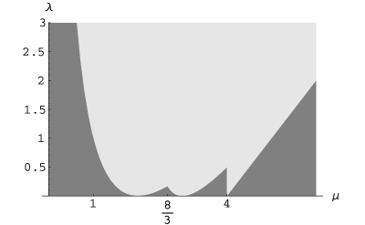
Figure 1: The light gray region is the subset of $\mathbb{R}^{+}\times\mathbb{R}^{+}$ of pairs $(\mu,\lambda)$ such that $V^{\mu}$ is unstable as a critical point of $E_{g_{\lambda}}$. The stability domain is painted in dark gray.

For spheres of upper dimension, we can use the vector fields $C_{2s}$ introduced in the previous section and we can also, following the idea used to solve the problem in dimension $3$, construct vector fields $A=a_{1}A_{a}+a_{2}A_{Ja}$, with $a_{1}$ and $a_{2}$ simultaneous eigenfunctions of the Laplacian and of the vertical Laplacian. With these directions we can improve the results stayed in [6], but unfortunately, it is not sufficient to solve the problem.