Turbulence measurements from H i absorption spectra

Abstract

We use the millennium Arecibo 21 cm absorption-line survey measurements to examine the issue of the non-thermal contribution to the observed Galactic H i line widths. If we assume a simple, constant pressure model for the H i in the Galaxy, we find that the non-thermal contribution to the line width, $v_{nt}$ scales as $v^{2}_{nt}\propto l^{\alpha}$, for $v_{nt}$ larger than $\sim 0.7$ km s^-1. Here $l$ is a derived length scale and $\alpha\sim 0.7\pm 0.1$. This is consistent with what one would expect from a turbulent medium with a Kolmogorov scaling. Such a scaling is also predicted by theoretical models and numerical simulations of turbulence in a magnetized medium. For non-thermal line widths narrower than $\sim 0.7$ km s^-1, this scaling breaks down, and we find that the likely reason is ambiguities arising from Gaussian decomposition of intrinsically narrow, blended lines. We use the above estimate of the non-thermal contribution to the line width to determine corrected H i kinetic temperature. The new limits that we obtain imply that a significantly smaller ($\sim 40\%$ as opposed to 60%) fraction of the atomic interstellar medium in our Galaxy is in the warm neutral medium phase.

1 Introduction

The classical description of the Galactic atomic interstellar medium (ISM) is that it consists of the cold neutral medium (CNM) and the warm neutral medium (WNM), in rough pressure balance with each other (e.g. Field, 1965; Field et al., 1969; Wolfire et al., 2003). Detailed modeling of the energy balance in a multi-phase medium (e.g. Wolfire et al., 1995) shows that the pressure equilibrium can be maintained for H i in one of two stable ranges of kinetic temperature (T_K), viz. $\sim 40$K $-200$K for the CNM and $\sim 5000$K $-8000$ K for the WNM. H i at intermediate temperatures is unstable and is expected to quickly migrate into one of the stable phases, unless energy is intermittently being injected into the medium. Recent observations and simulations indicate that in our Galaxy a significant fraction of the atomic ISM is in the thermally unstable region (e.g. V$\acute{a}$zquez-Semadeni et al., 2000; Heiles, 2001; Hennebelle & Audit, 2007; Hennebelle et al., 2007).

The classical method of determining the temperature of the atomic ISM is to compare the H i 21 cm line in absorption towards a bright continuum source with the emission spectrum along a nearby line of sight. Assuming that the physical conditions are the same along both lines of sight, one can measure the spin temperature (T_S) (or excitation temperature) of the H i (see e.g. Kulkarni & Heiles, 1988, for details). While the H i spin temperature, strictly speaking, characterizes the population distribution between the two hyperfine levels of the hydrogen atom, it is often used as a proxy for the kinetic temperature of the gas. This is because, in high density regions, T_S is expected to be tightly coupled to the kinetic temperature via collisions, while in low density regions, resonant scattering of Lyman-$\alpha$ photons is generally expected to couple the spin temperature to the kinetic temperature (Field, 1958).

The 21 cm optical depth of the WNM is extremely low (typically $<10^{-3}$) which makes it very difficult to measure the H i absorption from gas in the WNM phase. Consequently, emission-absorption studies usually provide only a lower limit to T_S. If the particle and Lyman-$\alpha$ number densities are low, T_S could in turn be significantly lower than T_K. On the other hand, one could use the 21 cm emission line width to determine an upper limit to the kinetic temperature. The line width is an upper limit to the temperature because in addition to thermal motions of the atoms, both bulk motion of the gas (e.g. differential rotation) as well as turbulence contribute to the observed line width.

The presence of turbulence in the atomic ISM of our own Galaxy can be detected through, for e.g. the scale free nature of the power spectrum of the intensity fluctuations in H i 21 cm emission (Crovisier & Dickey, 1983; Green, 1993). In a turbulent medium, one would also expect the velocity dispersion to increase as a power of the length scale. Such a power law velocity width length scale scaling has been observed in the atomic ISM of the Large Magellanic Cloud (LMC) (Kim et al., 2007). To the best of our knowledge it has not been observed in the atomic ISM of our own Galaxy. In this paper we show that, assuming that the atomic ISM is in rough pressure equilibrium, the data from the millennium Arecibo 21 cm absorption-line survey (Heiles & Troland, 2003a, b) is consistent with a velocity-length scale relation of the form $\sigma^{2}_{v}\propto l^{\alpha}$. We also show that this scaling is, to zeroth order, consistent with that expected from turbulence in an medium with magnetic field of $\sim$ few $\mu$Gauss.

Once one has an estimate of the turbulent velocity contribution to the observed velocity width, one can correct for it, to derive a tighter limit to the kinetic temperature. We show that this correction leads to a substantially smaller fraction of the gas being in the WNM phase than if one does not take turbulence into account.

2 Data, Analysis and Results

Figure 1: N_HI – T_S plot for Gaussian components from the millennium Arecibo 21 cm absorption-line survey data. The filled squares are components detected both in emission and absorption and the empty squares are components detected only in emission giving a lower limit of T_S.

The data we use are taken from the millennium Arecibo 21 cm absorption-line survey and consist of emission and absorption spectra with a velocity resolution of $\sim 0.4$ km s^-1 towards a total of 79 background radio sources. The observational and analysis techniques are discussed in detail by Heiles & Troland (2003a) and the astrophysical implications are discussed in Heiles & Troland (2003b). A brief summary is that the absorption spectra were corrected for emission from gas in the telescope beam by interpolating multiple off-source spectra, after which both the emission and absorption spectra were modeled as a collection of multiple Gaussian components. For each component, the spin temperature, upper limits on kinetic temperature, column densities and velocities were derived using these fits. There are several systematic uncertainties in such an analysis, discussed for example in Heiles & Troland (2003a), in particular those associated with estimating and subtracting the emission, and the assumption that each Gaussian component is a physically distinct entity. While a more robust measurement of the absorption spectra can be done using interferometric observations (e.g. Kanekar et al., 2003), here we work with the fit parameters provided as part of the survey. All the systematic uncertainties relevant to the Arecibo millennium absorption survey hence also apply to our results.

The survey lists a total of 374 Gaussian components in the emission spectra towards the 79 continuum sources Out of these, 205 components are also detected in H i absorption and have T_S measurements. For 21 of these components either the spin temperature had to be set to zero (by hand) in order to attain convergence of the fit (Heiles & Troland, 2003a) or the upper limit of the kinetic temperature computed from the line width is less than the spin temperature (or the lower limit of the spin temperature). The derived parameters for these components are clearly unphysical, and we do not use them in our analysis. We are hence left with a total of 353 Gaussian components consisting of 188 components detected both in emission and absorption and 165 components detected only in emission. In Figure (1) is a scatter plot of the spin temperature T_S against the column density N_HI; filled points are components that have been detected in both emission and absorption while empty points are components that have been detected only in emission. It is clear from the plot that the survey did not detect much gas with T${}_{\rm S}\lesssim 10$ K.

For a homogeneous cloud at temperature $T$, the pressure $P=nkT$, with $n=$ N${}_{\rm HI}/l$, where N_HI is the column density and $l$ is the length of the cloud. Putting these together we have $l=$N${}_{\rm HI}kT/P$. For the CNM clouds detected in absorption, it is quite reasonable to assume that the kinetic temperature is the same as the spin temperature T_S. If we further assume that the pressure is roughly constant across clouds, then we have $l\propto$N_HI T_S. Though the density and temperature of neutral ISM vary over a few orders of magnitude, this assumption is justified because the pressure changes, in most of the cases, only by a factor of a few since the turbulence in the gas is at most transonic. Further, for these components, the non-thermal component of the line width is given by $v^{2}_{nt}\propto$ (T_Kmax $-$ T_S), where T_Kmax is the measured line width of this component. In Figure (2) we show a scatter plot of (T_Kmax $-$ T_S) against N_HIT_S, as discussed above, to zeroth order this can be regarded as a plot of non thermal velocity against length scale. The solid line in the figure is a dual power law fit; at large length scales (log(N_HIT_S) $\geq 21.4\pm 0.2$) the power law index is $0.7\pm 0.1$, while at small length scales, the power law index is consistent with zero. The dotted line shows a fit which assumes that the measured T_Kmax is larger than the true T_Kmax by 60K; it provides a reasonable fit to the data over five orders of magnitude in N_HI T_S. The length scale corresponding to a pressure of 2000 cm^-3K, as well as the non thermal velocity width in km/s are also indicated in the figure.

The correlation between cloud scale length and the non-thermal line width that we see at long length scales is consistent with a turbulence driven velocity line-width relation. The assumptions we have made (viz. homogeneous clouds, constant pressure) are fairly naive, and are certainly not exactly valid in the current situation. The large scatter around the fit would be partly due to a break down of the assumptions (e.g. variations in the pressure) and partly due to measurement errors. If variations in pressure were the dominant contribution to the scatter, one would expect to see a systematic variation of the scatter plot for components in different Galactic latitude ranges. However, no such variation is seen.

Figure 2: N_HIT_S – T${}_{{\rm K}max}-$ T_S plot for Gaussian components from the millennium Arecibo 21 cm absorption-line survey data. Components detected both in emission and in absorption are only shown here. The solid line is a fit to the data using two power laws. The dotted line is the model with a $60$ K overestimation of T_Kmax (see §2 for details).

The ISM is known to have clumpy density and velocity structures and is believed to be turbulent at scales ranging from au to kpc (Dieter et al., 1976; Larson, 1981; Deshpande et al., 2000). Incompressible hydrodynamic turbulence leads to the famous Kolmogorov scaling $\sigma^{2}_{v}\propto l^{2/3}$ (Kolmogorov, 1941), similar to what we see at large length scales. However, the Galactic ISM cannot be modeled simply as an incompressible fluid. Recent theoretical studies and numerical simulations have investigated in details the turbulence of multi-phase medium (Koyama & Inutsuka, 2002; Audit & Hennebelle, 2005; Gazol et al., 2005; V$\acute{a}$zquez-Semadeni et al., 2006; Hennebelle et al., 2007). In some of these cases(V$\acute{a}$zquez-Semadeni et al., 2006; Hennebelle et al., 2007), synthetic H i spectra are computed to study the effect of turbulence. In general, these analytical and numerical works predict a Kolmogorov-like turbulence in two-phase neutral ISM. Hennebelle et al. (2007) also report, based on simulation results, a power law scaling $\sigma^{2}_{v}\propto l^{0.8}$ consistent with our observation.

Now, since fractional ionization couples the H i to the magnetic field, the turbulence is expected to be magnetohydrodynamic (MHD) in nature. Though simple and ingenious models (e.g. Goldreich & Sridhar, 1995) of incompressible MHD turbulence have been proposed, most of the insights into incompressible and compressible MHD turbulence again come from numerical simulations (Cho et al., 2002, and references therein). Models (like Goldreich & Sridhar, 1995) predict a Kolmogorov-like energy spectrum, $E(k)\propto k^{-5/3}$, for incompressible MHD turbulence and this is supported by both numerical simulations and observations (see Cho et al. (2002) for details). In case of compressible MHD turbulence, Alfv$\acute{e}$n modes are least susceptible to damping mechanisms (Minter & Spangler, 1997) and hence the energy transfer in Alfv$\acute{e}$n waves is of major interest. Again, numerical simulations show that the energy spectra of Alfv$\acute{e}$n modes follow a Kolmogorov-like spectrum.

In a situation where the bulk of the energy transfer is via Alfv$\acute{e}$n waves, the non-thermal velocity dispersion $\delta v$ is related to the magnetic perturbation amplitude $\delta B$ and H i number density $n_{H}$ as $\delta v=\delta B/\sqrt{4\pi\mu n_{\rm H}m_{\rm H}}$ (Arons & Max, 1975; Roshi, 2007) where $\mu=1.4$ is the effective mass of an H+He gas with cosmic abundance, $m_{\rm H}$ is the mass of the hydrogen atom and it is usually assumed that $\delta B\sim B$. Using this relation, the magnetic field is found to be of the order of few $\mu$G (column density weighted mean and median values are 11.7 and 10.2 $\mu$G respectively) with no significant trend related to “cloud” size. We note that there are various uncertainties to the derived equipartition magnetic field. But our estimate is broadly consistent with the observed magnetic field in the diffuse neutral ISM and matches, within a factor of 2, with the median magnetic field estimated for a sub-sample of these components using Zeeman splitting measurements (Heiles & Troland, 2005).

The break that is clearly seen in Figure (2) requires some attention. This change in the power law index can not be explained just in terms of lower signal to noise on the physical quantities at low N_HIT_S end. However, as shown in the figure, the data are well fit by a model in which the line width is overestimated by about $\sim 60$ K. There are three systematic effects that may contribute to the overestimation of the line width without much affecting N_HI and T_S: (i) the finite spectral resolution, (ii) blending of two or more narrow components and (iii) velocity (but not T_S) fluctuations in the gas within the Arecibo beam. The contribution from the first effect is quantified by estimating the width of a Gaussian signal after smoothing it to a spectral resolution of 0.4 km s^-1 and adding noise similar to that in the actual spectra. The effect is found to be almost negligible because of the high spectral resolution. A similar numerical exercise with two Gaussian components was done to check the effect of blending of narrow components and ambiguities in Gaussian fitting. In this case, the effect is most significant when the blended lines are of comparable amplitudes and have separations comparable to their widths. For example, blending of components with T${}_{\rm K}max=60$ K (width of the Gaussian $\sim 0.7$ km s^-1) with a separation of $\sim 1.2$ km s^-1 results in typically 20 – 30 K overestimation of T${}_{\rm K}max$. When the amplitudes of two Gaussian profiles are comparable, the line width is overestimated by upto $\sim 60$ K. The third possibility, that is, a fine scale structure in the velocity (but not in the temperature) has been proposed earlier (e.g. Brogan et al., 2005; Roy et al., 2006) to explain the observed fine scale H i opacity fluctuations (Dieter et al., 1976; Crovisier et al., 1985). Such velocity fluctuations within the Arecibo beam will also cause an overestimation of T${}_{\rm K}max$. We, however, note that the scale length (inferred from N_HI and T_S) of the components below the break is very small. Although the existence of tiny “clouds” is supported by observations and numerical simulations (Braun & Kanekar, 2005; Stanimirovi$\acute{c}$ & Heiles, 2005; Nagashima et al., 2006; V$\acute{a}$zquez-Semadeni et al., 2006; Hennebelle & Audit, 2007, e.g.), their origin and physical properties are still unknown. The evaporation timescale for these clouds are $\sim 1$ Myr. These structures can survive if either the ambient pressure around the clouds is much higher than the standard ISM pressure or they are formed continuously with a comparable timescale. While we have presented plausible arguments for the break that we see not corresponding to a physical phenomena, the lack of detailed understanding of these tiny H i structures means that we can not rule out the possibility of some physical phenomenon being responsible for the break.

2.1 A new indicator of the temperature

Figure 3: N_HIT_S – T${}_{{\rm K}max}-$ T_S plot for Gaussian components from the millennium Arecibo 21 cm absorption-line survey data. Components detected only in emission and not in absorption are shown here and T_S is the lower limit for these components. The solid line is derived from the components detected both in emission and in absorption.

Figure 4: Histogram of derived temperatures T_L and T_K. The solid lines only include components detected both in emission and in absorption and the dotted lines include all the components. The top two panels give the number of Gaussian components and the bottom panels give the H i column density. The left two panels are histogram of T_L and the right two are of T${}_{\rm K}max$.

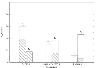
Figure 5: N_HI fraction, for components detected both in emission and in absorption (hatched histogram) and components detected only in emission and not in absorption (empty histogram), in different temperature range using T_L and T_Kmax as the proxy for the actual physical temperature.

For a multi-phase medium if the turbulent velocity dispersion scaling is similar for coexisting phases, then this scaling relation can be exploited to get a handle on the physical temperature of the gas that is detected only in H i emission but not in absorption. Since one only has a lower limit on T_S for these components, they lie, as expected, systematically on the top left side of the fit to the components detected in both emission and absorption (Figure (3)). For these components we define a proxy temperature T_L that will restore the component back to this power law correlation. Given the measured N_HI and T_Kmax from the emission spectra, one can uniquely compute this proxy temperature. Since T_L corresponds to the velocity width after correction for the turbulent velocity, it is a better estimate of the actual physical temperature of the cloud than that of T_Kmax. Note that since most of the components in Figure (3) line beyond the break in the fitted function the derived T_L is independent of the whether the break arises due to some underlying physical reason.

For all except 2 of the 165 components detected only in emission, T_L was calculated as described above. For two components, no meaningful solution for T_L could be found, and they are hence not included in the further analysis. For the components detected both in emission and in absorption, T_S is taken to be same as T_L. With this, we have T_L and T_Kmax for a total of 351 Gaussian components. Figure (4) shows the histogram of T_L and T_Kmax in terms of both number of “clouds” and H i column density. The top two panels give the number of Gaussian components and the bottom panels give the H i column density in different temperature bin. From the histograms, it is evident that our results qualitatively confirm the earlier detection of a significant fraction of gas in the thermally unstable region. Quantitatively, however, a significant fraction of the gas with high T_Kmax after correction for turbulent broadening corresponds to gas in the stable phase. This quantitative difference is illustrated in Figure (5) which shows the N_HI fraction for both the population (components detected both in emission and in absorption and components detected only in emission) in different temperature range using T_L instead of T_Kmax as the proxy for actual physical temperature. Further, while Heiles & Troland (2003b) find that $60\%$ of all H i is in the WNM phase, we find that only $40\%$ of the gas has temperature higher than $500$ K.

Figure 6: Histogram of derived temperatures for T${}_{\rm L}<500$ K. The solid lines only include components detected both in emission and in absorption and the dotted lines include all the components.

Figure 7: Histogram of scale length $L\sim$ N_HI T_S in terms of number of components (solid line) and total H i column density (dotted line). Two distinct peaks are evident in both cases.

A closer examination of the components with T${}_{\rm L}<500$ shows a clear peak near T${}_{\rm L}\sim 50$ K in the number distribution and that the major fraction of the gas is below T${}_{\rm L}\sim 100$ K as shown in Figure (6). Figure (7) shows the histogram of scale length $L\sim$ N_HI T_S. This clearly shows a bi-modal statistical distribution of the “cloud” size for the neutral ISM. As expected, the dominant contribution to the the peak at lower $L$ is from the cold components and to the peak at higher $L$ is mostly from the warm components. If $N$ is number of clouds along the lines of sight, $R$ is typical size of the clouds and $n$ is H i number density, then N(H i)${}_{X}\propto N_{X}R_{X}n_{X}$ where $X$ stands for CNM or WNM. From the observed N(H i) and $N$ for all the components used for this analysis we find, using this relation, $R_{\rm WNM}/R_{\rm CNM}\sim 110$ for typical $n_{\rm CNM}/n_{\rm WNM}\sim 100$. This is consistent with the ratio of the length scale corresponding to two peaks in the bi-modal distribution.

3 Conclusions

In this work we present a new phenomenology based technique to address the issue of non-thermal line width and the temperature of the diffuse neutral hydrogen of our Galaxy assuming a rough pressure equilibrium between different phases of the ISM. A possible connection between the observed Kolmogorov-like scaling of the non-thermal velocity dispersion in the Galactic H i and the turbulence of the interstellar medium is discussed. This scaling relation is used to re-examine the issue of the temperature of the Galactic ISM with the help of the millennium Arecibo 21 cm absorption-line survey measurements. The distribution of the derived temperature is found to be significantly different from the distribution of the upper limits of the kinetic temperature. A considerable fraction ($\sim 29\%$) of the gas is found to be in the thermally unstable phase, qualitatively confirming earlier results. However, about $60\%$ of all the neutral diffuse gas, a much higher fraction than that of reported earlier, has temperature below $500$ K. The CNM temperature distribution shows a clear peak near T $\sim 50$ K and the cloud size for the neutral ISM shows a bi-modal statistical distribution. Derived magnetic field from the non-thermal velocity dispersion matches, within a factor of 2, with the magnetic field value estimated from the Zeeman splitting measurements. The Kolmogorov-like scaling is consistent with the existing theoretical prediction, numerical simulations and earlier observational results.

References

- Audit & Hennebelle (2005) Audit E., Hennebelle P., 2005, A&A, 433, 1
- Abbott (1982) Abbott D. C., 1982, ApJ, 263, 723
- Arons & Max (1975) Arons J., Max C. E., 1975, ApJ, 196, L77
- Braun & Kanekar (2005) Braun R., Kanekar N., 2005, A&A, 436, L53
- Brogan et al. (2005) Brogan C. L., Zauderer B. A., Lazio T. J., Goss W. M., De Pree C. D., Fasion M. D., 2005, AJ, 130, 698
- Cho et al. (2002) Cho J., Lazarian A., Yan H., 2002, in Taylor A. R., Landecker T. L., Willis A. G., eds., Seeing Through the Dust: The Detection of H i and the Exploration of the ISM of Galaxies, San Francisco: Astronomical Society of the Pacific, Vol. 276, p.170
- Crovisier & Dickey (1983) Crovisier J., Dickey J. M., 1983, A&A, 122, 282
- Crovisier et al. (1985) Crovisier J., Dickey J. M., Kazs I., 1985, A&A, 146, 223
- Deshpande et al. (2000) Deshpande A. A., Dwarakanath K. S., Goss W. M., 2000, ApJ, 543, 227
- Dieter et al. (1976) Dieter N. H., Welch W. J., Romney J.D., 1976, ApJ, 206, L113
- Field (1958) Field G. B., 1958, Proc. IRE, 46, 240
- Field (1965) Field G. B., 1965, ApJ, 142, 531
- Field et al. (1969) Field G. B., Goldsmith D. W., Habing H. J., 1969, ApJ, 155, L149
- Gazol et al. (2005) Gazol A., Vzquez-Semadeni E., Kim J., 2005, ApJ, 630, 911
- Goldreich & Sridhar (1995) Goldreich P., Sridhar S., 1995, ApJ, 438, 763
- Green (1993) Green D. A., 1993, MNRAS, 262, 327
- Heiles (2001) Heiles C., 2001, ApJ, 551, L105
- Heiles & Troland (2003a) Heiles C., Troland T., 2003a, ApJS, 145, 329
- Heiles & Troland (2003b) Heiles C., Troland T., 2003b, ApJ, 586, 1067
- Heiles & Troland (2005) Heiles C., Troland T., 2005, ApJ, 624, 773
- Hennebelle & Audit (2007) Hennebelle P., Audit E., 2007, A&A, 465, 431
- Hennebelle et al. (2007) Hennebelle P., Audit E., Miville-Deschnes, M.-A., 2007, A&A, 465, 445
- Kanekar et al. (2003) Kanekar N., Subrahmanyan R., Chengalur J. N, Safouris V., 2003, MNRAS, 346, L57
- Kim et al. (2007) Kim S., et al., 2007, ApJS, 171, 419
- Kolmogorov (1941) Kolmogorov A., 1941, Dokl. Akad. Nauk SSSR, 31, 538
- Koyama & Inutsuka (2002) Koyama H., Inutsuka S., 2002, ApJ, 564, L97
- Kulkarni & Heiles (1988) Kulkarni S. R., Heiles C., 1988, in Verschuur G., Kellerman K., eds., Galactic and ExtraGalactic Radio Astronomy (2nd edition), Springer-Verlag, Berlin and New York, p95
- Larson (1981) Larson R. B., 1981, MNRAS, 194, 809
- Mac Low & Klessen (2004) Mac Low M., Klessen R. S., 2004, Rev. Mod. Phys., 76, 125
- McKee & Ostriker (1977) McKee C. F. , Ostriker J. P., 1977, ApJ, 218, 148
- Minter & Spangler (1997) Minter A., Spangler S., 1997, ApJ, 485, 182
- Nagashima et al. (2006) Nagashima M., Inutsuka S.-I., Koyama H., 2006, ApJ, 652, 41
- Roshi (2007) Roshi D. A., 2007, ApJ, 658, L41
- Roy et al. (2006) Roy N., Chengalur J. N., Srianand R., 2006, MNRAS, 365, L1
- Stanimirovi & Heiles (2005) Stanimirovi S., Heiles C., 2005, ApJ, 631, 371
- Vzquez-Semadeni et al. (2000) Vzquez-Semadeni E., Gazol A., Scalo J., 2000, ApJ, 540, 271
- Vzquez-Semadeni et al. (2006) Vzquez-Semadeni E., Ryu D., Passot T., Gonzlez R., Gazol A., 2006, ApJ, 643, 245
- Wolfire et al. (1995) Wolfire M. G., Hollenbach D., McKee C. F., Tielens A. G. G. M., Bakes E. L. O., 1995, ApJ, 443, 152
- Wolfire et al. (2003) Wolfire M. G., McKee C. F., Hollenbach D., Tielens A. G. G. M., 2003, ApJ, 587, 278