A Markov Process Inspired Cellular Automata Model of Departure Headways

Abstract

To provide a more accurate description of the driving behaviors in vehicle queues, a namely Markov-Gap cellular automata model is proposed in this paper. It views the variation of the gap between two consequent vehicles as a Markov process whose stationary distribution corresponds to the observed distribution of practical gaps. The multiformity of this Markov process provides the model enough flexibility to describe various driving behaviors. Two examples are given to show how to specialize it for different scenarios: usually mentioned flows on freeways and start-up flows at signalized intersections. The agreement between the empirical observations and the simulation results suggests the soundness of this new approach.

I Introduction

Traffic flow is a many-body system of strongly interacting vehicles. Various models are presented to understand the observed rich variety of physical phenomena exhibited by traffic flow ChowdhurySantenSchadschneider2000 , Helbing2001 , MahnkeKaupuzsLubashevsky2005 . From the viewpoint of vehicles’ queuing dynamics, these models generally depict four kinds of traffic flows: 1) static queues (e.g. vehicles parked on a line Lee2004 , RawalRodgers2005 , KernerKlenovHillerRehborn2006 , Abul-Magd2006 , and vehicle queues fully-stopped in front of signalized intersections JinSuZhangLi2008 ), 2) stable moving queues (vehicle platoons) which includes the well-known Kerner’s synchronized flow and wide-moving jams Kerner2004 , 3) free-flows formulating no explicit queues, and 4) unstable queues which contains complex inter-arrival and inter-departure queuing interactions HelbingTreiberKesting2006 , SchonhofHelbing2007 .

The queues with complex interactions between its elements attract increasing attentions recently. In many known approaches, the dynamics of flows are described on $N$ strongly-linked particles under fluctuations Helbing2001 , MahnkeKaupuzsLubashevsky2005 . Since the governing interaction forces or potentials are not directly measurable for traffic flow applications, the statistical distributions of particles are often investigated instead. For example, the important phase transition phenomena of traffic flow were studied by using scattering theory in HelbingTreiberKesting2006 , KrbalekHelbing2004 . Differently in Abul-Magd2007 , random matrix theory was applied to predict the space-gap distribution between vehicles in three-phrase flows. However, these studies focus on the steady-state statistics. Two questions thus arise as: 1) can we design microscopic simulation models (e.g. car-following, cellular automata) that meanwhile yields such statistical properties; 2) how to depict the transient-state statistics of inter-arrival and inter-departure queuing interactions. This paper aims to propose a simple yet useful CA model to partly answer these two questions.

In the field of traffic flow modeling, cellular automata (CA) based microscopic traffic simulation has received constant interests in the last decade, because of its efficiency on fast simulation and ability to imitate the driving behaviors to explain some complex phenomena MaerivoetMoor2005 . However, many CA models are designed to study the phase transitions of traffic flow only, i.e. NagelScheckenberg1992 , HelbingSchreckenberg1999 . The rather low accuracy on vehicles’ velocity and acceleration, which is useful in computer implementations, prevents them to incorporate further more features.

To deal with this problem, a new CA model is proposed in this paper. It models the variation of the gap between two consequent vehicles as Markov process, whose stationary distribution can be designed to reflect the distribution of empirical gap data. Because it is a dynamic model, it can simulate the inter-arrival and inter-departure queuing interactions, too. Moreover, the velocity adjusting rule can be gotten in a concise and unified way, which contains no intractable formulations and fits for fast simulations.

To prove its soundness, this general model is specialized to explain the interesting phenomena of traffic breakdown of freeway traffic flow and departure headways at signalized intersections. The agreement between the empirical and simulation results indicates that this new model approvingly reveals the implicit interactions between queuing vehicles. The results also prove the statement given in HelbingTreiberKesting2006 that the interdeparture time statistics is dominated by spatial interactions among the elements in a queue rather than the arrival or exit processes for a relatively long queue.

II The Markov-Gap CA Model

The model proposed here is a multi-cell CA model on a unidirectional, single-lane lattice, in which a vehicle is allowed to span a number of consecutive cells in the longitudinal direction; see Fig. 1. Multi-cell type is chosen here for modeling the possible small gaps during slow moving scenarios.

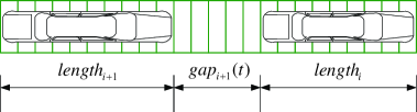
Figure 1: Diagram of the mutil-cell CA model.

Usually, CA models of road traffic contain two modes: free-driving mode, following/ braking mode. In the following/braking mode, a driver adjusts his/her vehicle to keep an as close as possible but not too close distance gap. Due to various reasons (inability to predict the leader’s action or make precise driving actions, possibility to be absent minded, etc.), he/she cannot maintain a constant gap. Suppose altogether we have $N$ possible gaps whose lengthes range from $0$ cell to $(N-1)$ cells. If at time $t$, the length of the gap is $n$; at the next time $(t+1)$, the length may still remain $n$, or possibly change to an adjacent value, i.e. $(n-1)$, $(n+1)$, etc.

Abstractly, this variation process of a gap during following can be viewed as a transferring process between $N$ states, where each state denotes a distinct gap in length. Statistically, considering the relatively long-time driving behaviors of many drivers, the transferring probability from state $i$ to $j$ would approach a steady value. That is, the drivers’ car-following actions can be depicted by a Markov Chain characterizing the variation process of gap. To our best knowledge, only SonKimLee2005 proposed a state-transition model similar to this model in a vague way, but it does not mention the Markov transferring probability.

Notice that the above Markov Chain is positive recurrent and aperiodic, it yields a steady-state (stationary) distribution, which straightforwardly corresponds to the empirical distributions of gap distance in traffic flow applications Luttinen1992 , MichaelLeemingDwyer2000 . This makes the model able to yield expected statistical features on gap/headways.

Indeed, it is not required to discretize the steady-state distribution into the minimal division level (the length of a cell here), because to consider too many transition states would be unnecessary and time consuming. In this paper, the so called Markov Chain Aggregation technique used in Stewart1994 , Spears1999 , BolchGreinerdeMeerTrivedideMeerTrivedi2006 is employed to combine some neighboring states and thus simplify transition matrix. Without losing much generality, we can further assume that a state (may span a number of consecutive cells) can only transfer to itself or the strictly neighboring state (noticing the simulation time span is usually short and the speed is limited, this assumption is reasonable). Thus, the transition matrix of the Markov Chain can be written into a tridiagonal matrix as:

$$\left[\begin{array}[]{cccccc}r_{0}&q_{0}&0&0&\cdots&0\\ p_{1}&r_{1}&q_{1}&0&\cdots&0\\ 0&p_{2}&r_{2}&q_{2}&&\vdots\\ \vdots&&&&&\vdots\\ 0&\cdots&\cdots&0&p_{n-1}&r_{n-1}\\ \end{array}\right]$$ (1)

where $p_{i}$, $r_{i}$, $q_{i}$ are the probabilities that transfer from state $i$ to the lower, current and higher states, respectively.

Let $p_{0}=q_{n-1}=0$, we have

$$p_{i}+r_{i}+q_{i}=1$$ (2)

for $i\in\{0,1,...,N-1\}$.

As well known, there exist numerous solutions for the potential transition matrix (1). Clearly any a valid solution could be used for simulation, but we generally have two more requirements for constructing Markov Chain for simulations: 1) lower time complexity of the formulation algorithm; and 2) faster convergency speed of the obtained Markov Chain, since it determines how many rounds of simulations are needed before drawing a satisfactory conclusion Stewart1994 , MeynTweedie1994 . To meet these two requirements, we can formulate such a matrix construction problem into a Semidefinite Programming (SDP) problem (e.g. SDP-(19) in BoydDiaconisXiao2004 ), which is easy to solve. In the rest of this paper, let’s assume the associated transition matrices (1) have already been obtained, since how to derive such a matrix does not accord with the main theme here.

Suppose the gap between the $(i-1)$th and $i$th vehicle is in the $n$th state at time $t$, which indicates that the gap of the $i$th vehicle satisfies $g_{i}(t)\in[g_{n}^{low},g_{n}^{up}]$. Here, $g_{n}^{low}$ and $g_{n}^{up}$ denote the lower and upper boundaries of the $n$th state, respectively.

Based on the above Markov transition idea, the gap might be enlarged into the $(n+1)$th state with probability $q_{n}$ due to deceleration. In the simulation, an arbitrary random number $\widetilde{g_{i}^{+}}(t+1)$ will be uniformly generated in $[g_{n+1}^{low},g_{n+1}^{up}]$ and assigned as the potential forthcoming gap. And the expected velocity $v_{i}$ of the $i$th vehicle at time $(t+T)$ should be

$$\widetilde{v_{i}^{-}}(t+T)=v_{i-1}(t)-[\widetilde{g_{i}^{+}}(t)-g_{i}(t)]/T$$ (3)

Similarly, when acceleration, the velocity should be adjusted as

$$\widetilde{v_{i}^{+}}(t+T)=v_{i-1}(t)-[\widetilde{g_{i}^{-}}(t)-g_{i}(t)]/T$$ (4)

where $\widetilde{g_{i}^{-}}(t)\in[g_{n-1}^{low},g_{n-1}^{up}]$.

Noticing most CA models of road traffic consists of an accelerating rule to make the vehicle approach the highest possible speed and a braking rule to avoid collisions, we can similarly write the whole updating rules as:

1) If $g_{i}(t)>G_{max}$, where $G_{max}$ denotes the maximum coupling distance; the vehicle is in free-driving scheme, then it will approach the highest velocity as

$$v_{i}(t+T)=\min\{v_{i}(t)+a_{max}^{+}\times T,v_{max}\}$$ (5)

Else if $v_{i}(t)-v_{i-1}(t)>[g_{i}(t)-G]/H$, there exists a risk to collide, and thus let the vehicle brake

$$v_{i}(t+T)=v_{i}(t)-D\times T$$ (6)

where $G$, $H$ and $D$ are constants denoting the minimum safety gap, deceleration time and braking decelerating rate, respectively.

Otherwise, the velocity of the vehicle is updated as follows, where the $\max$, $\min$ functions are added to guarantee that the velocity and ac/decelerating rates are within the limits.

$$v_{i}(t+T)=\left\{\begin{array}[]{ll}\min\{v_{i}(t)+a_{max}^{+}\times T,\widetilde{v_{i}^{+}}(t+T),v_{max}\}&\textrm{, with $p_{n}$}\\ v_{i}(t)&\textrm{, with $r_{n}$}\\ \max\{v_{i}(t)-a_{max}^{-}\times T,\widetilde{v_{i}^{-}}(t+T),0\}&\textrm{, with $q_{n}$}\par\end{array}\right.$$ (7)

2) The position of vehicle is then updated as

$$x_{i}(t+T)=x_{i}(t)+v_{i}(t)\times T$$ (8)

Simulations show that the multiformity of this Markov process provides the model enough flexibility to describe diversified driving behaviors. The transferring matrix can be explicitly determined by the investigation data from drivers or implicitly estimated through the observed distribution of gap.

However, the above model should not be directly applied, if the velocity of vehicles varies in a relatively large range. This is primely because drivers would like to keep a roughly constant time headway instead of gap distance. (As shown in KernerKlenovHillerRehborn2006 , Abul-Magd2007 , the time-headway distributions computed for the free-flow, synchronized flow, and moving jam traffic phases do not differ too much in shape and mean values.) Usually, the larger the velocity is, the larger the gap distance should be. Thus, the aforementioned transition matrix (1)) should be modified to be velocity-dependent in such situations. Examples of implementing this trick will be shown in the coming sections.

III A Specialization for Flows on Freeways

To illustrate the effectiveness of the proposed model, a specialized form is used to reproduce spontaneous traffic breakdowns and moving jams that have been observed for flows on freeways. The velocity of a vehicle may vary significantly in such situations. However, to assign a Markov matrix (1) for each velocity (more precisely to make the model into a time-dependent continuous time Markov process) is troublesome for fast simulations; thus the aggregation idea is used again.

Suppose we only consider $J$ Markov Chains, each of which corresponds to a certain range of velocity. When the velocity of the $i$th vehicle $v_{i}(t)$ fall into the $j$th velocity range at time $t$, we will apply the $j$th Markov transition matrix in velocity updating. In the following simulation, five transition matrices are designed (in a sense to the five speed stages of a car); see Fig. 2. All the five distributions are uniformly discretized histogram ($5$ segments, $3.3$m per segment for velocity range $[0,9]$; $4$ segments, $4.1$m per segment for velocity range $[9,18]$; and $3$ segment, $5.5$m per segment for the rests). The discretized stationary distributions are assigned as Table. 1 with respect to the practical observations HelbingTreiberKesting2006 , SchonhofHelbing2007 , Abul-Magd2007 . The associated $v_{max}$ in (5) and (7) are also set the $9$m/s, $18$m/s, …, for each range respectively.

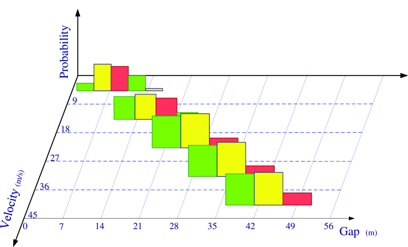
Figure 2: The assumed discretized steady-state gap distributions according to different velocities.

Table 1: The discretized gap distributions according to different velocities.

Index	Velocity range(m/s)	Gap range(m)	Probability in each segment
1	[0,9]	[0.5,17]	[0.10,0.35,0.32,0.20,0.03]
2	[9,18]	[9,25.5]	[0.30,0.33,0.28,0.09]
3	[18,27]	[18,34.5]	[0.42,0.45,0.13]
4	[27,36]	[27,43.5]	[0.41,0.0.45,0.14]
5	[36,54]	[36,52.5]	[0.41,0.43,0.16]

Here, the length of each cell is set as $0.1$m. The length of each vehicle is uniformly set as 4m. The maximum coupling distance between two consecutive vehicles is set as $52.5$m, which means the follower will enter free navigation mode if the gap to its leader is greater than $52.5$m.

The velocity is updated once $T=1$s. The maximum velocity of a vehicle is set to $v_{max}=45$m/s, the maximum accelerating rate is $a_{max}^{+}=7.5$m/s², and the maximum decelerating rate is $a_{max}^{-}=15$m/s². A fully stopped vehicle will start to move only if the gap ahead is greater than $2.2$m. And the braking parameters are set as $G=0.5$m, $H=7$s, $D=15$m/s².

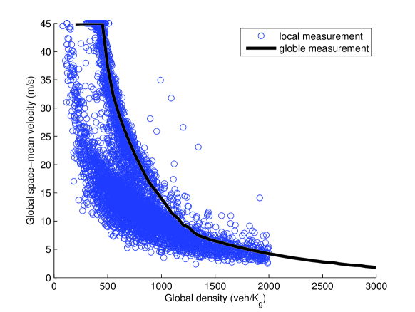
Figure 3: The $(k,\bar{v}_{s})$ diagram for the proposed model, obtained by local and global measurements.

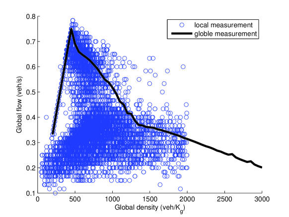
Figure 4: The $(k,q)$ diagram for the proposed model, obtained by local and global measurements.

Fig. 3 and Fig. 4 show the $(k,\bar{v}_{s})$ and $(k,q)$ diagrams for the proposed model, obtained by local and global measurements. These microscopic traffic stream characteristics are measured according to MaerivoetMoor2005 . Here, $K_{g}$ denotes the length of the closed single-lane system, which is $27000$m. It can be seen from Fig. 3 that the local measurements interestingly tend to form clusters around certain space-mean velocities, which corresponds to the so called optimal velocities predicated in Bando1995 , HelbingTilch1998 , JiangWuZhu2001 . These clusters appear as branches in Fig. 4, too. This indicates that the most important merit of the optimal velocity models has been inherited by the proposed model, though via a different interpretation of the dynamical equilibrium between traffic flow velocity and density. Moreover, it yields the right headway distribution as observed other than that given in Fig.7 of Bando1995 .

Besides, the local measurements in Fig. 4 also discriminate Kerner’s three-phase flows: the free-flow regime contains only a few data points on line starts from the original point; the synchronized regime is visible as a wide scatter of the data points, having various speeds but relatively high flows; and synchronized-flow, and jammed regimes contains the data points in the wide-moving jam correspond to Kerner’s line $J$. Thus, the proposed model can reproduce the traffic phenomena of phase transitions formation observed in real traffic.

It should be pointed out that the highest flow rate of the proposed model is larger than that of NaSch model NagelScheckenberg1992 , mainly because of the different settings of vehicle’s length.

IV Another Specialization for Start-up Flow at Signalized Intersections

Another specialization is proposed in this section to explain the distributions of the observed departure headway. Results indicate that the proposed model can also depict the transient-state statistics of unstable queues.

Departure headways are usually defined as the times that elapse between consecutive vehicles when vehicles in a queue start crossing the stop line (or any other reference line) at a signalized intersection after the light turns green. Modeling departure headways at signalized intersections attracts constant research efforts due to its importance. Most previous works focus on the mean departure headways of the first tens of vehicles. The results show that the headways tend to decrease sequentially as queue position increases, and a steady headway will be reached since the fourth or the fifth vehicle, i.e. Luttinen1992 , MichaelLeemingDwyer2000 , ChangZhangMaoGong2005 . Further investigations shows that each of these departure headways follows a log-normal distribution (whose logarithm is normally distributed) respectively and their mean values decrease to a saturation value gradually LiWang2006 , SuWeiChengYaoZhangLiZhangLi2008 ; see Fig. 5.

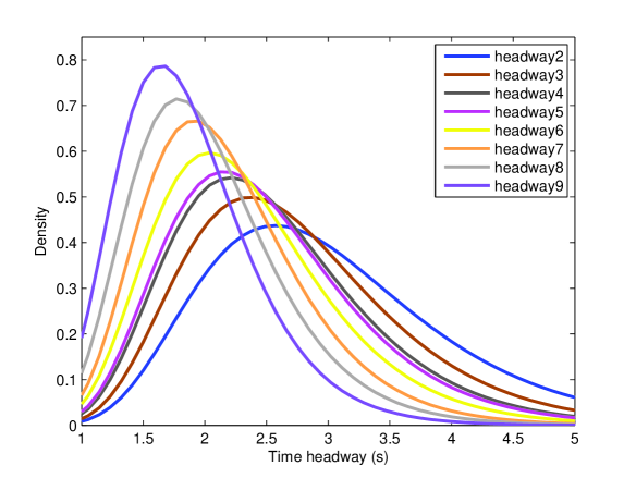
Figure 5: The empirical distributions of departure headways identified from the histograms observed. The departure headway data used here are collected from several intersections in Beijing, China during 2006 to 2007 by using video cameras. The recording time is from 9:00 AM to 10:00 AM, when the traffic flow is not too crowded. The queuing length does not grow so long (typically $5\sim 9$ vehicles) in this period.

Only the movements of the first few vehicles, which are fully stopped when the light turns green, are recorded and examined. The vehicles whose length is too long (more than 10m) are discarded as well as their following vehicles. The sample sizes decrease according to the positions due to this data pre-processing process. The statistics of the observed departure headways are listed in Table. 2. Kolmogorov-Smirnov (K-S) hypothesis test is used here to check whether the empirical distributions are similar to the estimated log-normal distributions, and Jarque-Bera (J-B) hypothesis test is used to check the departure of the distribution of empirical headways’ logarithm from normality Gardiner1983 . The criteria level is set as 95%, which means the hypothesis will be accepted if the value is greater than 0.05.

Table 2: The Kolmogorov-Smirnov (K-S) and Jarque-Bera (J-B) hypothesis testing results of empirical departure headways. $\mu$ and $\sigma$ denote the mean and standard deviation of the logarithm of data respectively.

Postion	Sample size	K-S test	J-B test	$\mu$	$\sigma$
2	423	0.4282	0.2730	1.0569	0.3353
3	423	0.3788	0.3089	0.9639	0.3210
4	422	0.1684	0.3028	0.8920	0.3171
5	416	0.3050	0.3157	0.8701	0.3163
6	394	0.4635	0.3657	0.8089	0.3127
7	298	0.3261	0.1849	0.7372	0.2991
8	146	0.8587	0.1060	0.6670	0.2996
9	42	0.8544	0.5000	0.5849	0.2945

By specializing the above Markov-Gap CA model, we can give a explanation of such phenomena. Here, the length of each cell is set as $0.1$m. The length of each vehicle is still $4$m. Here, only four transition matrices are designed; see Fig. 6. All the four distributions are uniformly discretized into 9 states (9 segments, $2$m per segment) discretized histogram. If the velocity of a vehicle lies in $[0,4]$m/s, then the gap variation process is assumed to follows the log-normal distribution with mean $1.9$ and stand deviation $0.8$. After discretizing, the allowable gap range is divided into $9$ monospaced states between $2$m to $20$m. Similarly, we have the other settings as shown in Table. 3. The maximum coupling distance between two consecutive vehicles is set as $27$m.

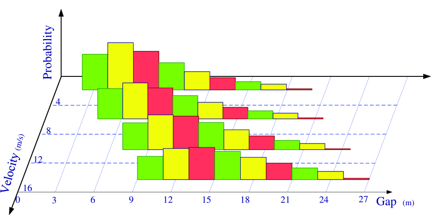
Figure 6: The assumed discretized steady-state gap distributions according to different velocities.

Table 3: The designed discretized log-normal type gap distributions according to different velocities. $\bar{\mu}$ and $\bar{\sigma}$ denote the mean and standard deviation of the logarithm of data respectively.

Index	Velocity range(m/s)	Gap range(m)	$\bar{\mu}$	$\bar{\sigma}$
1	[0,4]	[2,20]	1.9	0.8
2	[4,8]	[4,22]	2.2	0.7
3	[8,12]	[7,25]	2.5	0.5
4	[12,16]	[9,27]	2.7	0.45

The initial gaps of the vehicles are assigned as random numbers following a normal distribution ($\mu_{initgap}=1.7$m, $\sigma_{initgap}=0.1$). The velocity is updated once $T=0.50\sim 0.70$s randomly, because human drivers usually cannot make decision or take action in a too short time). The maximum velocity of a vehicle is set to $v_{max}=16$m/s here, and the maximum ac/decelerating rate is $a_{max}^{+}=a_{max}^{-}=6$m/s². And the braking parameters are set as $G=0.5$m, $H=12.5$s, $D=6$m/s².

Before the simulation, all the vehicles are fully stopped. And the departure of a vehicle starts one by one (a vehicle will start to move only if the gap ahead is greater than $2.2$m). The first vehicle will steadily accelerate to $16$m/s in the $16$s (accelerating rate $1$m/s²) and then keep this speed.

Results below show that the resulting mean departure headways (400 rounds of simulations for several times) following a similar but faster decreasing pattern to the empirical ones; see Fig. 7. The statistics of a set of simulated departure headways are given in Table. 4 (the criteria level is still 95%). The simulated headways do not decrease exactly like empirical ones, partly because: 1) the empirical samples for the last few positions are limited and may be biased, 2) the simple braking rule (5) is still not accurate enough to depict the real tracking dynamics. More efforts will be put into here for better concordance between the empirical and simulated data. However, it is apparent that this model captures the main features of the driving behaviors in a discharging queue and therefore yields an accordant macroscopic statistic result through a minimal description of their microscopic interactions.

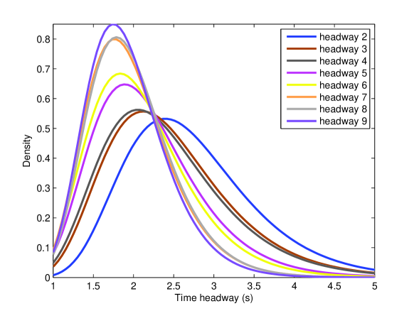
Figure 7: The distributions of a typical set of departure headways identified from the histograms obtained in simulation

Table 4: The Kolmogorov-Smirnov (K-S) and Jarque-Bera (J-B) hypothesis testing results of a typical set of simulated departure headways $\hat{\mu}$ and $\hat{\sigma}$ denote the mean and standard deviation of the logarithm of data respectively.

Postion	Sample size	K-S test	J-B test	$\hat{\mu}$	$\hat{\sigma}$
2	400	0.7525	0.0325	0.9623	0.2993
3	400	0.3678	0.0501	0.8540	0.3211
4	400	0.6651	0.0706	0.8283	0.3268
5	400	0.5992	0.2564	0.7336	0.3104
6	400	0.7980	0.3834	0.6992	0.3035
7	400	0.8780	0.1100	0.6413	0.2726
8	400	0.6681	0.7080	0.6520	0.2673
9	400	0.0912	0.1979	0.6265	0.2595

Further simulations also reveal that:

1) The general shapes of the simulated departure headways distributions will be roughly kept according to different aggregation ratio, unless the number of states is too small. This proves the Markov Chain Aggregation technique in (1) is applicable.

2) The variation trend of mean departure headways is not very sensitive to the initial positions and velocities of the vehicles, which fits the facts observed.

- (1) D. Chowdhury, L. Santen, A. Schadschneider, Phys. Rep. 329, 199 (2000).
- (2) D. Helbing, Rev. Mod. Phys. 73, 1067 (2001).
- (3) R. Mahnke, J. Kaupuzs, I. Lubashevsky, Phys. Rep. 408, 1 (2005).
- (4) J. W. Lee, Physica A 331, 531 (2004).
- (5) S. Rawal, G. J. Rodgers, Physica A 346, 621 (2005).
- (6) B. S. Kerner, S. L. Klenov, A. Hiller, and H. Rehborn, Phys. Rev. E 73, 046107 (2006).
- (7) A.Y. Abul-Magd, Physica A 368, 536 (2006).
- (8) X. Jin, Y. Su, Y. Zhang, L. Li, arXiv:0803.2619
- (9) B. S. Kerner, The Physics of Traffic (Springer, Heidelberg, 2004).
- (10) D. Helbing, M. Treiber, A. Kesting, Physica A 36, 62 (2006).
- (11) M. Schonhof, D. Helbing, Transp. Sci. 41, 135 (2007).
- (12) M. Krbalek, D. Helbing, Physica A 333, 370 (2004).
- (13) A. Y. Abul-Magd, Phys. Rev. E 76, 057101 (2007).
- (14) S. Maerivoet, B. De Moor, Phys. Rep. 419, 1 (2005).
- (15) K. Nagel, M. Schreckenberg, J. Phys. I 2, 2221 (1992).
- (16) D. Helbing, M. Schreckenberg, Phys. Rev. E 59, 2505 (1999).
- (17) B. Son, T. Kim, T. Lee, in Lecture Notes in Computer Science 3481, 863 (2005).
- (18) R. T. Luttinen, Transp. Res. Rec. 1365, 92 (1992).
- (19) P. G. Michael, F. C. Leeming, W. O. Dwyer, Transp. Res. F, 3, 55 (2000).
- (20) W. J. Stewart, Introduction to the Numerical Solution of Markov Chains, (Princeton University Press, Priceton, 1994).
- (21) W. M. Spears, in Proceedings of the Congress on Evolutionary Computation, (1999).
- (22) G. Bolch, S. Greiner, H. de Meer, K. S. Trivedi, H. de Meer, K. S. Trivedi, Queueing Networks and Markov Chains: Modeling and Performance Evaluation with Computer Science Applications, 2nd ed., (John Wiley and Sons, 2006).
- (23) S. P. Meyn, R. L. Tweedie, Markov Chains and Stochastic Stability, (Springer-Verlag, New York, 1993).
- (24) S. Boyd, P. Diaconis, and L. Xiao, SIAM Review 46, 667 (2004).
- (25) M. Bando, K. Hasebe, A. Nakayama, A. Shibata, Y. Sugiyama, Phys. Rev. E, 51, 1035 (1995).
- (26) D. Helbing, B. Tilch, Phys. Rev. E 58, 133 (1998).
- (27) R. Jiang, Q. S. Wu, Z. J. Zhu, Phys. Rev. E 64, 017101 (2001).
- (28) Y. Chang, P. Zhang, L. Mao, Z. Gong, in Proceedings of Traffic and Granular Flow 05, (2005).
- (29) L. Li, F. Wang, in Lecture Notes in Computer Science 4153, 105 (2006).
- (30) Y. Su, Z. Wei, S. Cheng, D. Yao, Y. Zhang, L. Li, Z. Zhang, Z. Li, in Transportation Research Board Annual Meeting CD, (2008).
- (31) C. W. Gardiner, Handbook of Stochastic Methods for Physics, Chemistry and the Natural Sciences, (Springer-Verlag, New York, 1983).