PROPERTIES OF THE REISSNER–NORDSTRÖM SPACETIMES
WITH A NONZERO COSMOLOGICAL CONSTANT

Abstract

Properties of the Reissner–Nordström black-hole and naked-singularity spacetimes with a nonzero cosmological constant $\Lambda$ are represented by their geodetical structure and embedding diagrams of the central planes of both the ordinary geometry and associated optical reference geometry. Both the asymptotically de Sitter ($\Lambda>0$) and anti-de Sitter ($\Lambda<0$) spacetimes are considered and compared with the asymptotically flat ($\Lambda=0$) spacetimes. Motion of test particles (timelike geodesics for uncharged particles) and photons (null geodesics) is described in terms of an appropriate ‘effective potential.’ Circular geodesics are discussed and photon escape cones are determined. The spacetimes are divided in their parameter space into separated parts according to different character of the effective potential and properties of the circular geodesics. In all asymptotically anti-de Sitter black-hole spacetimes and some asymptotically de Sitter black-hole spacetimes a region containing stable circular geodesics exists, which allows accretion processes in the disk regime. On the other hand, around some naked singularities, both asymptotically de Sitter and anti-de Sitter, even two separated regions with stable circular geodesics exist. The inner region is limited from below by particles with zero angular momentum that are located in stable equilibrium positions. The inertial and gravitational forces related to the optical reference geometry are introduced and specified for the circular motion. It is shown how the properties of the centrifugal force are closely related to the properties of the optical reference geometry embedding diagrams.

145 Institute of Physics, Faculty of Philosophy and Science, Silesian University in Opava, Bezručovo nám. 13, CZ-746 01 Opava, Czech Republic June 12, 2002

1 Introduction

Recently acquired data from a wide range of cosmological tests, including the measurements of the present value of the Hubble parameter and dynamical estimates of the present energy density of the Universe, measurements of the anisotropy of the cosmic relict radiation, statistics of gravitational lensing of quasars and active galactic nuclei, galaxy number counts, and measurements of high-redshift supernovae, indicate convincingly that in the framework of the inflationary paradigm, a very small relict repulsive cosmological constant $\Lambda>0$, or an analogous concept of quintessence, has to be invoked in order to explain the dynamics of the recent Universe [1, 2, 3, 4, 5, 6]. The presence of a repulsive cosmological constant changes dramatically the asymptotic structure of black-hole backgrounds. Such backgrounds become asymptotically de Sitter spacetimes, not flat spacetimes.

On the other hand, the anti-de Sitter spacetimes play a crucial role in the framework of superstring theories [7, 8]. Therefore, it is also important to obtain information on the influence of an attractive cosmological constant ($\Lambda<0$) on the structure of black-hole backgrounds.

It is crucial to understand the role of a nonzero cosmological constant in astrophysically relevant situations. For these purposes, analysis of geodetical motion is among the most fundamental techniques. Further, the curvature of the spacetime under consideration can be conveniently demonstrated by using embedding diagrams of 2-dimensional, appropriately chosen, spacelike surfaces into 3-dimensional Euclidean space [9]. The 3-dimensional optical reference geometry [10] associated with the geometry of the spacetime under consideration enables a natural ‘Newtonian’ concept of gravitational and inertial forces and reflects some hidden properties of the geodetical motion [11]. Usually, the embedding diagrams of appropriately chosen 2-dimensional sections of the optical reference geometry directly illustrate properties of the centrifugal force [12, 13, 14, 15, 16].

Both the geodetical structure and embedding diagrams were studied extensively in the Schwarzschild–de Sitter and Schwarzschild–anti-de Sitter spacetimes [14]. However, all of these spacetimes containing a static region are black-hole spacetimes. Clearly, it is useful to have an idea of the influence of a nonzero cosmological constant on the character of naked-singularity spacetimes, too.

Naked singularities, i.e., spacetime singularities not hidden behind an event horizon, represent solutions to the Einstein equations for the most exotic compact gravitational objects that could be conceivable to explain quasars and active galactic nuclei. The Penrose conjecture of cosmic censorship [17] suggests that no naked singularity evolves from regular initial data, however, the proof and even precise formulation of the conjecture still stands as one of the biggest challenges in general relativity. Therefore, it seems important to consider possible astrophysical consequences of the hypothetical existence of naked singularities. Of particular interest are those effects that could distinguish a naked singularity from black holes. We shall consider the influence of a nonzero cosmological constant on the character of the simplest, spherically symmetric naked singularity spacetimes containing a nonzero electric charge $Q$.

We know a wide class of solutions of the Einstein equations representing naked singularities. Here, we focus our attention to the simplest class of solutions of the Einstein–Maxwell equations with $\Lambda\neq 0$ that describe both naked-singularity and black-hole spacetimes.These solutions are given by the spherically symmetric Reissner–Nordström–(anti-)de Sitter spacetimes. Using standard methods, we shall study geodetical motion in these spacetimes and embedding diagrams of the central planes of both the ordinary space geometry and optical reference geometry. The results will be compared with known related properties of both the Schwarzschild–(anti-)de Sitter black-hole spacetimes ($Q=0$) and Reissner–Nordström spacetimes black-hole and naked-singularity spacetimes ($\Lambda=0$).

The paper is organized in the following way. In Section 2, the Reissner–Nordström–(anti-)de Sitter spacetimes are separated into the black-hole and naked-singularity spacetimes in the parameter space. In Section 3, the geodetical motion is discussed for test particles and photons. In Section 4, photon escape cones are established from the properties of the null geodesics. In Section 5, embedding diagrams of the central planes of the ordinary space geometry are constructed and the limits of embeddability are given. In Section 6, the optical reference geometry is introduced, and the inertial and gravitational forces related to the optical geometry are defined and expressed for general circular motion, i.e., the motion with $r=\mathrm{const}$, $\theta=\mathrm{const}$. In Section 7, embedding diagrams of the central planes of the optical geometry are constructed. The limits of embeddability are given and the turning points of the embedding diagrams are related to the properties of the centrifugal force. In Section 8, asymptotic behavior of the optical geometry near the black-hole horizons and the cosmological horizon is discussed. In Section 9, new features of the geodetical motion and the embedding diagrams, caused by the interplay of the electric charge of the background and a nonzero cosmological constant in both the black-hole and naked-singularity spacetimes, are summarized and briefly discussed.

2 Classification of the Reissner–Nordström spacetimes with a nonzero cosmological constant

In the standard Schwarzschild coordinates $(t,r,\theta,\phi)$, and the geometric units ($c=G=1$), the Reissner–Nordström–de Sitter ($\Lambda>0$), and Reissner–Nordström–anti-de Sitter ($\Lambda<0$) spacetimes are given by the line element

$$\mathrm{d}s^{2}= - \left(1-\frac{2M}{r}+\frac{Q^{2}}{r^{2}}-\frac{\Lambda}{3}r^{2}\right)\mathrm{d}t^{2}+\left(1-\frac{2M}{r}+\frac{Q^{2}}{r^{2}}-\frac{\Lambda}{3}r^{2}\right)^{-1}\mathrm{d}r^{2}$$ (1)

$$+ r^{2}\left(\mathrm{d}\theta^{2}+\sin^{2}\theta\,\mathrm{d}\phi^{2}\right),$$

and the related electromagnetic field is given by the four-potential

$$A_{\mu}=\frac{Q}{r}\,\delta_{\mu}^{t}.$$ (2)

Here, $M$ denotes mass and $Q$ denotes electric charge of the spacetimes. However, it is convenient to introduce a dimensionless cosmological parameter

$$y\equiv\textstyle\frac{1}{3}\Lambda M^{2},$$ (3)

a dimensionless charge parameter

$$e\equiv\frac{Q}{M},$$ (4)

and dimensionless coordinates $t\to t/M$, $r\to r/M$. It is equivalent to putting $M=1$.

The event horizons of the geometry (1) are determined by the condition

$$-g_{tt}\equiv 1-\frac{2}{r}+\frac{e^{2}}{r^{2}}-y{r^{2}}=0.$$ (5)

The loci of the event horizons can be expressed as solutions of the equation

$$y=y_{\mathrm{h}}(r;e)\equiv\frac{r^{2}-2r+e^{2}}{r^{4}}.$$ (6)

Inspecting properties of the function $y_{\mathrm{h}}(r;e)$, we determine distribution of black-hole and naked-singularity spacetimes in the parameter space ($e^{2}$-$y$).

In the special case of $e=0$, the black-hole spacetimes exist for all $y\leq 0$, and for $0<y\leq y_{\mathrm{c}}=1/27$. If $y>1/27$, a naked singularity exists, however, there is no static region in these spacetimes (for details, see Ref. [14]).

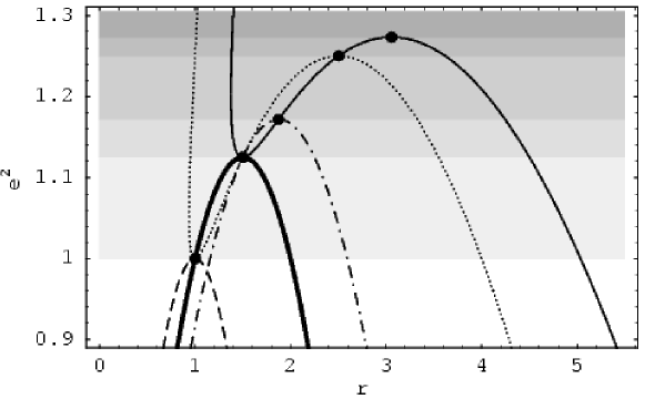
Figure 1: The characteristic functions governing the test-particle geodetical motion in the Reissner–Nordström–(anti-)de Sitter spacetimes. The function $e^{2}_{\mathrm{z(h)}}(r)$ (represented by the dashed curve) governs the zero points (event horizons of Reissner–Nordström black holes) and the characteristic function $e^{2}_{\mathrm{e(h)}}(r)$ (represented by the bold solid curve) governs the local extrema of the function $y_{\mathrm{h}}(r;e)$ determining the event horizons of the Reissner–Nordström–(anti-)de Sitter spacetimes. Their respective local maxima are located at the points $(1,1)$ and $(3/2,9/8)$. The characteristic functions $e^{2}_{\mathrm{z(ms)}\pm}(r)$ (represented by the dotted curve) govern the zero points of $y_{\mathrm{ms}}(r;e)$ determining the marginally stable circular geodesics, the characteristic function $e^{2}_{\mathrm{d(ms)}}(r)$ (represented by the dashed-dotted curve) governs the divergent points of $y_{\mathrm{ms}}(r;e^{2})$, and the characteristic functions $e^{2}_{\mathrm{e(ms)}\pm}(r)$ (represented by the thin solid curve) govern the local extrema of the function $y_{\mathrm{ms}}(r;e)$. Their respective local maxima are located at the points $(5/2,5/4)$ (on the ‘$-$’ branch), $(15/8,75/64)$ and $(55/18,275/216)$ (on the ‘$-$’ branch). The local minimum of the function $e^{2}_{\mathrm{z(ms)}\pm}(r)$ (the ‘$-$’ branch) coincides with the local maximum of the function $e^{2}_{\mathrm{z(h)}}(r)$ at (1,1), the local minimum of the function $e^{2}_{\mathrm{e(ms)}\pm}(r)$ (the ‘$-$’ branch) coincides with the local maximum of the function $e^{2}_{\mathrm{e(h)}}(r)$ at $(3/2,9/8)$. The extrema of the functions (depicted by bold dots) divide the nonnegative region of the parameter $e^{2}$ into six subintervals emphasized by increasing gray levels, each of them implying different behavior of the functions $y_{\mathrm{h}}(r;e)$ and/or $y_{\mathrm{ms}}(r;e)$.

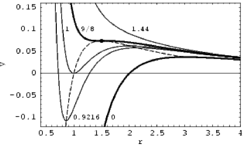
Figure 2: Loci of the event horizons in the Reissner–Nordström–(anti-)de Sitter spacetimes. The functions $y_{\mathrm{h}}(r;e^{2})$ depicted in the figure are labeled by the corresponding value of the parameter $e^{2}$. For $e^{2}=0$, the corresponding function (represented by the lower bold curve) diverge to $-\infty$ as $r\to 0_{+}$. Three qualitatively different cases of behavior of the function $y_{\mathrm{h}}(r;e^{2})$ for $e^{2}>0$ can be distinguished. For $0<e^{2}<9/8$, one local minimum and one local maximum occur on the function $y_{\mathrm{h}}(r;e^{2})$, moreover, $y_{\mathrm{h}}(r;e^{2})>0$ if $1<e^{2}<9/8$. For $e^{2}=9/8$, both extrema merge in the inflex point (depicted by the bold dot) located at $(3/2,y_{\mathrm{crit}}=2/27)$ on the critical curve (represented by the upper bold curve), and for $e^{2}>9/8$ the function $y_{\mathrm{h}}(r;e^{2})$ is monotonically decreasing. The loci of the local extrema are emphasized by the dashed curve.

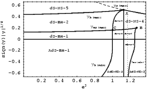
Figure 3: The classification of the Reissner–Nordström–(anti-)de Sitter spacetimes according to properties of the effective potential of the test-particle geodetical motion. The functions $y_{\mathrm{h(min)}}(e^{2})$ and $y_{\mathrm{h(max)}}(e^{2})$ limit the region of black-hole spacetimes (shaded) in the parameter space $e^{2}$-$y$. Outside that region, merely naked-singularity spacetimes exist. The function $y_{\mathrm{s(max)}}(e^{2})$ (represented by the dashed curve in the region, where it is irrelevant for the classification) marks the local maxima of the function $y_{\mathrm{s}}(r;e^{2})$ governing the static radii. The functions $y_{\mathrm{ms(min)}}(e)$ and $y_{\mathrm{ms(max)}}(e)$ separate the asymptotically de Sitter black-hole spacetimes containing a region of stable circular orbits allowing accretion processes in the disk regime (dS-BH-1) from those with unstable circular orbits only (dS-BH-2), and the naked-singularity spacetimes with two regions of stable circular orbits from those with one region of stable circular orbits (see the text and Figs 5 and 7). The relevant points have the following coordinates $e^{2}$ and $y$: $A(9/8,2/27)$, $B(275/216,0.001753)$, $C(1.000695,0.0006931)$. Notice that in order to make the distribution of different classes in the parameter space more evident, we use the function $\mathop{\operator@font sign}\nolimits(y)|y|^{1/4}$.

For $e^{2}>0$, properties of $y_{\mathrm{h}}(r;e^{2})$ can be reviewed in the following way. The zero points are given by the relation determining horizons of Reissner–Nordström black holes

$$e^{2}=e^{2}_{\mathrm{z(h)}}\equiv 2r-r^{2}.$$ (7)

There is one divergent point at $r=0$, where $y_{\mathrm{h}}(r\to 0,e^{2})\to+\infty$. The asymptotic behavior is given by $y_{\mathrm{h}}(r\to\infty,e^{2})\to 0$. The local extrema (given by $\partial y_{\mathrm{h}}(r;e^{2})/\partial r=0$) are determined by the relation

$$e^{2}=e^{2}_{\mathrm{e(h)}}\equiv\textstyle\frac{1}{2}(3r-r^{2}).$$ (8)

Both function $e^{2}_{\mathrm{z(h)}}(r)$, $e^{2}_{\mathrm{e(h)}}(r)$ are drawn in Fig. 1. At the local extrema, the cosmological parameter is given by the relations

$$y_{\mathrm{h(max)}}(e) \equiv \frac{r_{\mathrm{e(h)}+}-e^{2}}{r^{4}_{\mathrm{e(h)}+}},$$ (9)

$$y_{\mathrm{h(min)}}(e) \equiv \frac{r_{\mathrm{e(h)}-}-e^{2}}{r^{4}_{\mathrm{e(h)}-}},$$ (10)

where

$$r_{\mathrm{e(h)}\pm}=\frac{3}{2}\left[1\pm\left(1-\frac{8e^{2}}{9}\right)^{1/2}\right].$$ (11)

Clearly, the local extrema can exist, if $e^{2}\leq e^{2}_{\mathrm{crit}}=9/8$. For $e^{2}=9/8$, $y_{\mathrm{h}}(r;e^{2})$ has an inflex point at $r=3/2$, with value of the cosmological parameter

$$y=y_{\mathrm{crit}}\equiv\textstyle\frac{2}{27}$$ (12)

corresponding to the largest value of $y$ that permits the existence of black-hole solutions. We can distinguish three qualitatively different cases of behavior of $y_{\mathrm{h}}(r;e^{2})$ (see Fig. 2) according to the charge parameter $e^{2}$. Properties of the Reissner–Nordström–(anti-)de Sitter spacetimes relatively to the parameter $y$, $e^{2}$ can then be classified easily.

If $0<e^{2}\leq 1$, there is $y_{\mathrm{h(min)}}<0$; if $1<e^{2}\leq 9/8,y_{\mathrm{h(min)}}>0$; if $e^{2}>9/8$, there are no local extrema.

The black-hole spacetimes (with $e^{2}<9/8$) can exist just if $y_{\mathrm{h(min)}}(e)<y<y_{\mathrm{h(max)}}(e)$; for $y<y_{\mathrm{h(min)}}(e)$ or $y>y_{\mathrm{h(max)}}(e)$, the naked-singularity spacetimes occur. Clearly, for $e^{2}>9/8$ naked-singularity spacetimes exist only, while for $1<e^{2}<9/8$ no black holes can exist in asymptotically anti-de Sitter spacetimes. Both black-hole and naked-singularity spacetimes in both asymptotically de Sitter and anti-de Sitter universe can exist if $0<e^{2}\leq 1$. In asymptotically de Sitter spacetimes ($y>0$), a black-hole geometry has three horizons $r_{\mathrm{b}-}<r_{\mathrm{b}+}<r_{\mathrm{c}}$. The geometry is static under the inner black-hole horizon ($0<r<r_{\mathrm{b}-}$), and between the outer black-hole and cosmological horizons ($r_{\mathrm{b}+}<r<r_{\mathrm{c}}$). In asymptotically anti-de Sitter spacetimes ($y<0$), a black hole geometry has two horizons $r_{\mathrm{b}-}<r_{\mathrm{b}+}$, and the geometry is static under the inner horizon ($0<r<r_{\mathrm{b}-}$) and above the outer horizon ($r>r_{\mathrm{b}+}$). The relations (9) and (10) directly yield the distribution of black-hole and naked-singularity spacetimes in the space of parameters $y$ and $e^{2}$ (see Fig. 3)

3 Geodetical motion

Motion of uncharged test particles and photons is governed by the geodetical structure of the spacetime. The geodesic equation reads

$$\frac{\mathrm{D}p^{\mu}}{\mathrm{d}\lambda}=0,$$ (13)

where $p^{\mu}\equiv\mathrm{d}x^{\mu}/\mathrm{d}\lambda$ is the four-momentum of a test particle (photon) and $\lambda$ is the affine parameter related to the proper time $\tau$ of a test particle by $\tau=\lambda/m$. The normalization condition reads

$$p^{\mu}p_{\mu}=-m^{2},$$ (14)

where $m$ is the rest mass of the particle; $m=0$ for photons.

It follows from the central symmetry of the geometry (1) that the geodetical motion is allowed in the central planes only. Due to existence of the time Killing vector field $\mathchoice{\mbox{\boldmath$\displaystyle\xi$}}{\mbox{\boldmath$\textstyle\xi$}}{\mbox{\boldmath$\scriptstyle\xi$}}{\mbox{\boldmath$\scriptscriptstyle\xi$}}_{(t)}=\partial/\partial t$ and the axial Killing vector field $\mathchoice{\mbox{\boldmath$\displaystyle\xi$}}{\mbox{\boldmath$\textstyle\xi$}}{\mbox{\boldmath$\scriptstyle\xi$}}{\mbox{\boldmath$\scriptscriptstyle\xi$}}_{(\phi)}=\partial/\partial\phi$, two constants of the motion must exist, being the projections of the four-momentum onto the Killing vectors:

$$p_{t} = g_{t\mu}p^{\mu}=-\mathscr{E},$$ (15)

$$p_{\phi} = g_{\phi\mu}p^{\mu}=\Phi.$$ (16)

In the spacetimes with $\Lambda\neq 0$, the constants of motion $\mathscr{E}$ and $\Phi$ cannot be interpreted as energy and axial component of the angular momentum at infinity since the geometry is not asymptotically flat. However, it should be interesting to discuss a possibility to find regions of these spacetimes with character ‘close’ to the asymptotic regions of the Schwarzschild (or Reissner–Nordström) spacetimes.

It is convenient to introduce specific energy $E$, specific axial angular momentum $L$ and impact parameter $\ell$ by the relations

$$E=\frac{\mathscr{E}}{m},\quad L=\frac{\Phi}{m},\quad\ell=\frac{\Phi}{\mathscr{E}}.$$ (17)

Choosing the plane of the motion to be the equatorial plane ($\theta=\pi/2$ being constant along the geodesic), we find that the motion of test particles ($m\neq 0$) can be determined by an ‘effective potential’ of the radial motion

$$V^{2}_{\mathrm{eff}}(r;L,y,e)\equiv\left(1-\frac{2}{r}+\frac{e^{2}}{r^{2}}-yr^{2}\right)\left(1+\frac{L^{2}}{r^{2}}\right).$$ (18)

Since

$$(u^{r})^{2}=\left(\frac{\mathrm{d}r}{\mathrm{d}\tau}\right)^{2}=E^{2}-V^{2}_{\mathrm{eff}}(r;L,y,e),$$ (19)

the motion is allowed where

$$E^{2}\geq V^{2}_{\mathrm{eff}}(r;L,y,e),$$ (20)

and the turning points of the radial motion are determined by the condition $E^{2}=V^{2}_{\mathrm{eff}}(r;L,y,e)$.

The radial motion of photons ($m=0$) is determined by a ‘generalized effective potential’ $\ell^{2}_{\mathrm{R}}(r;y,e)$ related to the impact parameter $\ell$. The motion is allowed, if

$$\ell^{2}\leq\ell^{2}_{\mathrm{R}}(r;y,e)\equiv\frac{r^{4}}{r^{2}-2r+e^{2}-yr^{4}},$$ (21)

the condition $\ell^{2}=\ell^{2}_{\mathrm{R}}(r,y,e)$ gives the turning points of the radial motion.

The special case of $e=0$ has been extensively discussed in Ref. [14]. Therefore, we concentrate our discussion on the case $e^{2}>0$. The effective potentials $V^{2}_{\mathrm{eff}}(r;L,y,e)$ and $\ell^{2}_{\mathrm{R}}(r;y,e)$ define turning points of the radial motion at the static regions of the Reissner–Nordström–(anti-)de Sitter spacetimes. (At the dynamic regions, where the inequalities $V_{\mathrm{eff}}(r;L,y,e)<0$ and $\ell^{2}_{\mathrm{R}}(r;y,e)<0$ hold, there are no turning points of the radial motion). $V^{2}_{\mathrm{eff}}$ is zero at the horizons, while $\ell^{2}$ diverges there. At $r=0$, $V^{2}_{\mathrm{eff}}\to+\infty$, while $\ell^{2}_{\mathrm{R}}=0$. Circular orbits of uncharged test particles correspond to local extrema of the effective potential ($\partial V_{\mathrm{eff}}/\partial r=0$). Maxima ($\partial^{2}V_{\mathrm{eff}}/\partial r^{2}<0$) determine circular orbits unstable with respect to radial perturbations, minima ($\partial^{2}V_{\mathrm{eff}}/\partial r^{2}>0$) determine stable circular orbits. The specific energy and specific angular momentum of particles on a circular orbit, at a given $r$, are determined by the relations

$$E_{\mathrm{c}}(r;y,e) = \frac{1-\frac{2}{r}+\frac{e^{2}}{r^{2}}-yr^{2}}{\left(1-\frac{3}{r}+\frac{2e^{2}}{r^{2}}\right)^{1/2}},$$ (22)

$$L_{\mathrm{c}}(r;y,e) = \left(\frac{r-e^{2}-yr^{4}}{1-\frac{3}{r}+\frac{2e^{2}}{r^{2}}}\right)^{1/2}.$$ (23)

(The minus sign for $L_{\mathrm{c}}$ is equivalent to the plus sign in spherically symmetric spacetimes, therefore, we do not give the minus sign explicitly here and in the following.)

At $r=r_{\mathrm{ph}+}$, and $r=r_{\mathrm{ph}-}$, where

$$r_{\mathrm{ph}\pm}(e)=\frac{3}{2}\left[1\pm\left(1-\frac{8e^{2}}{9}\right)^{1/2}\right],$$ (24)

both $E_{\mathrm{c}}$ and $L_{\mathrm{c}}$ diverge—photon circular orbits exist at these radii. The photon circular orbits are determined by the local extrema of the function $\ell^{2}_{\mathrm{R}}(r;y,e)$, which are located at $r=r_{\mathrm{ph}\pm}(e)$ independently of the cosmological parameter $y$. Of course, the impact parameter of the photon circular orbits depends on $y$; there is

$$\ell^{2}_{\mathrm{c}\pm}(y,e)=\frac{r^{4}_{\mathrm{ph}\pm}}{r^{2}_{\mathrm{ph}\pm}-2r_{\mathrm{ph}\pm}+e^{2}-yr^{4}_{\mathrm{ph}\pm}}.$$ (25)

The loci of photon circular orbits can be implicitly given by the equation $e^{2}=e^{2}_{\mathrm{ph}}(r)=e^{2}_{\mathrm{e(h)}}$. Because $r_{\mathrm{ph}\pm}(e)=r_{\mathrm{e(h)}\pm}(e)$, where $r_{\mathrm{e(h)}\pm}(e)$ determine local extrema of the function $y_{\mathrm{h}}(r;e)$ governing horizons of the Reissner–Nordström–(anti-)de Sitter spacetimes, we can directly conclude that two photon circular orbits can exist at the naked-singularity spacetimes with $y<y_{\mathrm{h(min)}}(e)$, while one photon circular orbit at $r_{\mathrm{ph}+}(e)>r_{\mathrm{b}+}(e)$ exists in the black-hole spacetimes with $y_{\mathrm{h(min)}}(e)<y<y_{\mathrm{h(max)}}(e)$. If no local extrema of $y_{\mathrm{h}}(r;e)$ exist, i.e., for $0<e^{2}\leq 9/8$ and $y>y_{\mathrm{h(max)}}(e)$, and for $e^{2}>9/8$ and $y$ arbitrary, no photon circular geodesics are admitted in the corresponding naked-singularity spacetimes.

The circular geodesics are allowed at regions, where the denominator of both (22) and (23) is real, i.e., at

$$r<r_{\mathrm{ph}-}\quad\mathrm{and}\quad r>r_{\mathrm{ph}+}.$$ (26)

However, we have to add the condition given by reality of the numerator in Eq. (23):

$$r-e^{2}-yr^{4}\geq 0.$$ (27)

The equality at (27) determines so called static radii $r_{\mathrm{s}}$, where $L_{\mathrm{c}}(r_{\mathrm{s}};y,e)=0$.

The static radii are given by the condition

$$y=y_{\mathrm{s}}(r;e)\equiv\frac{r-e^{2}}{r^{4}}.$$ (28)

The asymptotic behavior of $y_{\mathrm{s}}(r,e)$ is determined by relations

$$y_{\mathrm{s}}(r\to 0,e)\to-\infty,\quad y_{\mathrm{s}}(r\to\infty,e)\to 0.$$ (29)

The function $y_{\mathrm{s}}(r;e)$ has its zero point at $r=e^{2}$ and its local maximum is at $r=4e^{2}/3$, where

$$y_{\mathrm{s(max)}}(e)=\frac{27}{256e^{6}}.$$ (30)

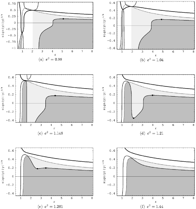
Figure 4: Properties of the circular geodesics in the Reissner–Nordström–(anti-)de Sitter spacetimes. Determined by the functions $y_{\mathrm{h}}(r;e)$ (thick solid lines), giving event horizons , $y_{\mathrm{ms}}(r;e)$ (thin solid lines), giving marginally stable circular orbits, and $y_{\mathrm{s}}(r;e)$ (dotted lines), giving so called static radii, where particles with zero angular momentum remain at an equilibrium position. According to the value of the charge parameter $e^{2}$, there are six qualitatively different classes of the behavior of the functions $y_{\mathrm{h}}(r;e)$, $y_{\mathrm{ms}}(r;e)$, $y_{\mathrm{s}}(r;e)$ (for details see text and Fig. 1), subsequently illustrated in cases (a) through (f). The circular orbits are limited by the function $y_{\mathrm{s}}(r;e)$, and by the radii $r_{\mathrm{ph}-}$, $r_{\mathrm{ph}+}$, corresponding to photon circular orbits existing in the spacetimes with $e^{2}<9/8$ [in cases (a) and (b)]. Regions admitting existence of circular geodesics are shaded. If the orbits are unstable, a low level of gray is used, while the regions of stable circular geodesics are emphasized by a higher level of gray.

The function $y_{\mathrm{s(max)}}(e)$ is illustrated in Fig. 3. The function $y_{\mathrm{s}}(r;e)$ has common points with the function $y_{\mathrm{h}}(r;e)$ at its extreme points $y_{\mathrm{h(min)}}(e)$, and $y_{\mathrm{h(max)}}(e)$. The behavior of $y_{\mathrm{s}}(r)$ is illustrated in qualitatively different cases in Fig. 4. The properties of static radii in dependence on the parameters $e$, $y$ can be summarized in the following way.

• $0<e^{2}\leq 1$  If $y<y_{\mathrm{h(min)}}$, there is one static radius at $r_{\mathrm{s}1}<r_{\mathrm{ph}-}$. If $0<y<y_{\mathrm{h(max)}}$, there is one static radius at $r_{\mathrm{s}2}>r_{\mathrm{ph}+}$.

• $1<e^{2}\leq 9/8$  If $y<0$, there is one static radius at $r_{\mathrm{s}1}<r_{\mathrm{ph}-}$. If $0\leq y<y_{\mathrm{h(min)}}$, there are two static radii at $e^{2}<r_{\mathrm{s}1}<r_{\mathrm{ph}-}$, $r_{\mathrm{s}2}>r_{\mathrm{ph}+}$. If $y_{\mathrm{h(min)}}\leq y<y_{\mathrm{h(max)}}$, there is one static radius at $r_{\mathrm{s}2}>r_{\mathrm{ph}+}$.

• $e^{2}>9/8$  If $y<0$, there is one static radius at $r_{\mathrm{s}1}<4e^{2}/3$. If $0\leq y<y_{\mathrm{s(max)}}$, there are two static radii at $e^{2}<r_{\mathrm{s}1}<4e^{2}/3<r_{\mathrm{s}2}$. If $y=y_{\mathrm{s(max)}}$ there is one static radius located at $r_{\mathrm{s}1}=r_{\mathrm{s}2}=4e^{2}/3$. If $y>y_{\mathrm{s(max)}}$ there are no static radii.

If $y>0$, the gravitational attraction of a black hole acting on a stationary particle is exactly balanced by the cosmological repulsion at the static radius; in the case of naked singularities, the balance occurs at two static radii if $e^{2}<9/8$ and $y<y_{\mathrm{h(min)}}(e)$, or if $e^{2}>9/8$ and $y<y_{\mathrm{s(max)}}(e)$. On the other hand, static radii do not exist for naked singularities with $e^{2}>9/8$ and $y>y_{\mathrm{s(max)}}(e)$. If $y<0$, there is no static radius in the black-hole spacetimes, and just one static radius in the naked-singularity spacetimes. Then the existence of the static radius indicates some gravitational repulsion connected with the influence of the charge parameter on the spacetime structure of the Reissner–Nordström–anti-de Sitter naked singularities. A similar effect occurs in the field of Kerr naked singularities [18].

The conditions (26) and (27) limiting radii of circular geodetical motion have to be considered simultaneously. We arrive at the conclusion that the geodetical circular orbits are allowed at radii

$$r_{\mathrm{s}1}<r<r_{\mathrm{ph}-},\quad r_{\mathrm{ph}+}<r<r_{\mathrm{s}2}.$$ (31)

The stable circular geodesics are limited by the relation

$$4yr^{6}-15yr^{5}+12ye^{2}r^{4}-r^{3}+6r^{2}-9e^{2}r+4e^{4}\leq 0.$$ (32)

Radii of the marginally stable circular geodesics, given by the equality in (32), can be expressed in the form

$$y=y_{\mathrm{ms}}(r;e)\equiv\frac{r^{3}-6r^{2}+9e^{2}r-4e^{4}}{r^{4}\left(4r^{2}-15r+12e^{2}\right)}.$$ (33)

The asymptotic behavior of the function $y_{\mathrm{ms}}(r;e)$ is given by the relations $y_{\mathrm{ms}}(r\to 0,e)\to-\infty$, $y_{\mathrm{ms}}(r\to\infty,e)\to 0$. The zero points of $y_{\mathrm{ms}}(r;e)$, determining marginally stable circular geodesics of the Reissner–Nordström spacetimes, are given by the relation

$$e^{2}=e^{2}_{\mathrm{z(ms)}}(r)\equiv\frac{9r\pm r\sqrt{16r-15}}{8},$$ (34)

while its divergent points are located at $r=0$, where $y_{\mathrm{ms}}(r\to 0,e)\to-\infty$, and at radii implicitly determined by the relation

$$e^{2}=e^{2}_{\mathrm{d(ms)}}(r)\equiv\frac{15r-4r^{2}}{12}.$$ (35)

Both functions $e^{2}_{\mathrm{z(ms)}}(r)$ and $e^{2}_{\mathrm{d(ms)}}(r)$ are illustrated in Fig. 1. The function $e^{2}_{\mathrm{z(ms)}}(r)$ has a local minimum at $r=1$, where $e^{2}=1$, and a local maximum at $r=5/2$, where $e^{2}_{\mathrm{z(ms)(max)}}=5/4$. The function $e^{2}_{\mathrm{d(ms)}}(r)$ has a local maximum at $r=15/8$, where there is $e^{2}_{\mathrm{d(ms)(max)}}=75/64$.

Local extrema of $y_{\mathrm{ms}}(r;e)$ determine the extremal values $y_{\mathrm{ms(max)}}(e)$ and $y_{\mathrm{ms(min)}}(e)$ of spacetimes that admit existence of stable circular geodesics. These local extrema are determined by the equation

$$(2e^{2}-3r+r^{2})(16e^{4}-28e^{2}r+15r^{2}-2r^{3})=0.$$ (36)

In the special case of $e=0$ , we find $r_{\mathrm{max}}=15/2$ and $y_{\mathrm{ms(max)}}=12/15^{4}\approx 0.000237$; further, there is $r_{\mathrm{min}}=3$ and $y_{\mathrm{ms(min)}}=1/27$, which is irrelevant for timelike geodesics (see Ref. [14] for details).

In the following we shall restrict our attention to the case of $e^{2}>0$. The common points of $y_{\mathrm{ms}}(r;e)$ and $y_{\mathrm{h}}(r;e)$ are located at $r=r_{\mathrm{ph}+}$ and $r=r_{\mathrm{ph}-}$, where both $y_{\mathrm{ms}}(r;e)$ and $y_{\mathrm{h}}(r;e)$ have local extrema, because of the first bracket of Eq. (36); these are also common points with the function $y_{\mathrm{s}}(r;e)$. Other local extrema of $y_{\mathrm{ms}}(r;e)$ are determined by the term in the second bracket in Eq. (36). They can be given by the relation

$$e^{2}=e^{2}_{\mathrm{e(ms)}\pm}(r)\equiv\frac{7r-r\sqrt{8r-11}}{8}.$$ (37)

The functions $e^{2}_{\mathrm{e(ms)}\pm}(r)$ are real at $r\geq 11/8$; at $r=11/8$ there is $e^{2}=77/64$. The function $e^{2}_{\mathrm{e(ms)}-}(r)$ has a zero point at $r_{\mathrm{z}}=15/2$ (corresponding to the Schwarzschild–de Sitter case), a local minimum at $r_{\mathrm{(e}-\mathrm{)min}}=3/2$, where $e^{2}_{\mathrm{e(min)}}=9/8$, and a local maximum at $r_{\mathrm{(e}-\mathrm{)max}}=55/18$, where $e^{2}_{\mathrm{e(max)}}=275/216$. The function $e^{2}_{\mathrm{e(ms)}\pm}(r)$ is, again, illustrated in Fig. 1. Inspecting Fig. 1 we can conclude that the local extrema of $y_{\mathrm{ms}}(r;e)$, determined by Eq. (37), govern only one local extreme of $y_{\mathrm{ms}}(r;e)$ in the spacetimes with black-hole horizons ($e^{2}<9/8$), while they govern three local extrema in naked-singularity spacetimes with $9/8<e^{2}<275/216$. Using Eqs (33) and (37), values of the cosmological parameter at these local extrema, $y_{\mathrm{ms(min)}}(e)$, and $y_{\mathrm{ms(max)}}(e)$ are determined and illustrated in Fig. 3.

It follows from the discussion presented above that properties of the circular geodesics in dependence on the charge parameter $e^{2}$ can be separated into six qualitatively different cases (see Fig. 1). They are illustrated in Fig. 4 giving qualitatively different behavior of the characteristic functions $y_{\mathrm{h}}(r;e)$, $y_{\mathrm{s}}(r;e)$, $y_{\mathrm{ms}}(r;e)$; we do not include the special case $e^{2}=0$—as it can be found in Ref. [14]. The six qualitatively different cases of the behavior of the characteristic functions are: (a) $0<e^{2}\leq 1$, (b) $1<e^{2}\leq 9/8$ [this interval needs a subdivision according to the relation of $y_{\mathrm{h(min)}}(e)$, and $y_{\mathrm{ms(max)}}(e)$; if $e^{2}<e^{2}_{\mathrm{eq}}=1.000695$, there is $y_{\mathrm{h(min)}}(e)<y_{\mathrm{ms(max)}}(e)\leq y_{\mathrm{ms(bh)}}(e^{2}_{\mathrm{eq}})=0.0006931$, while for $e^{2}>e^{2}_{\mathrm{eq}}$, there is $y_{\mathrm{h(min)}}(e)>y_{\mathrm{ms(max)}}(e)$], (c) $9/8<e^{2}<75/64$, (d) $75/64<e^{2}<5/4$, (e) $5/4<e^{2}<275/216$, (f) $e^{2}>275/216$. The circular geodesics are limited by relations (31), the lower branch of the circular geodesics ($r_{\mathrm{s}1}<r<r_{\mathrm{ph}-}$) can exist in naked-singularity spacetimes only. In the black-hole spacetimes no circular photon orbit can exist under the inner horizon. The stable circular orbits are limited by $y_{\mathrm{ms}}(r;e)$ from above outside the radii of divergence of this function. Between the radii of divergence, the stable circular orbits have to be limited by $y_{\mathrm{ms}}(r;e)$ from below—these regions are always irrelevant for timelike geodesics.

Analysis of the characteristic functions $y_{\mathrm{h}}(r;e)$, $y_{\mathrm{s}}(r;e)$, $y_{\mathrm{ms}}(r;e)$ shows that there are eleven types of the Reissner–Nordström–(anti-)de Sitter spacetimes with qualitatively different behavior of the effective potential of the geodetical motion (and the circular orbits). We shall define the types of the Reissner–Nordström spacetimes with a nonzero cosmological constant according to the properties of the circular geodesics, as they directly follow from Fig. 4.

dS-BH-1

(Type dS-BH-1 means asymptotically de Sitter black-hole spacetime of type 1; in the following, the notation has to be read in an analogous way.) One region of circular geodesics at $r>r_{\mathrm{ph}+}$ with unstable then stable and finally unstable geodesics (for radius growing).

dS-BH-2

One region of circular geodesics at $r>r_{\mathrm{ph}+}$ with unstable geodesics only.

dS-NS-1

Two regions of circular geodesics, the inner region consists of stable geodesics only, the outer one contains subsequently unstable, then stable and finally unstable circular geodesics.

dS-NS-2

Two regions of circular orbits, the inner one consist of stable orbits, the outer one—of unstable orbits.

dS-NS-3

One region of circular orbits, subsequently with stable, unstable, then stable and finally unstable orbits.

dS-NS-4

One region of circular orbits with stable and then unstable orbits.

dS-NS-5

No circular orbits allowed.

AdS-BH-1

One region of circular geodesics at $r>r_{\mathrm{ph}+}$ with unstable and then stable geodesics.

AdS-NS-1

Two regions of circular geodesics, the inner one $(r<r_{\mathrm{ph}-})$ consists of stable geodesics only, the outer one $(r>r_{\mathrm{ph}+})$ contains both unstable and then stable circular geodesics.

AdS-NS-2

One region of circular orbits, subsequently with stable, then unstable and finally stable orbits.

AdS-NS-3

One region of circular orbits with stable orbits exclusively.

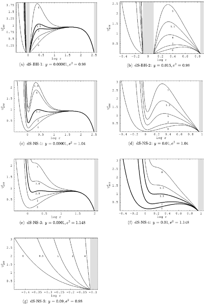
Figure 5: The effective potential $V^{2}_{\mathrm{eff}}(r;e,y,L)$ of the test-particle geodetical motion in the asymptotically de Sitter spacetimes. There are seven qualitatively different types of the behavior of $V^{2}_{\mathrm{eff}}$ (for details see text and Fig. 4), illustrated in the cases (a) through (g). The dynamic regions of the spacetimes, where $V^{2}_{\mathrm{eff}}$ is not well defined, are shaded. The curves representing the effective potential are labeled by values of the angular momentum $L$. Note that in the spacetimes dS-NS-1 and 2, the character of $V^{2}_{\mathrm{eff}}$ with the local maxima and minima is preserved for $L\to\infty$.

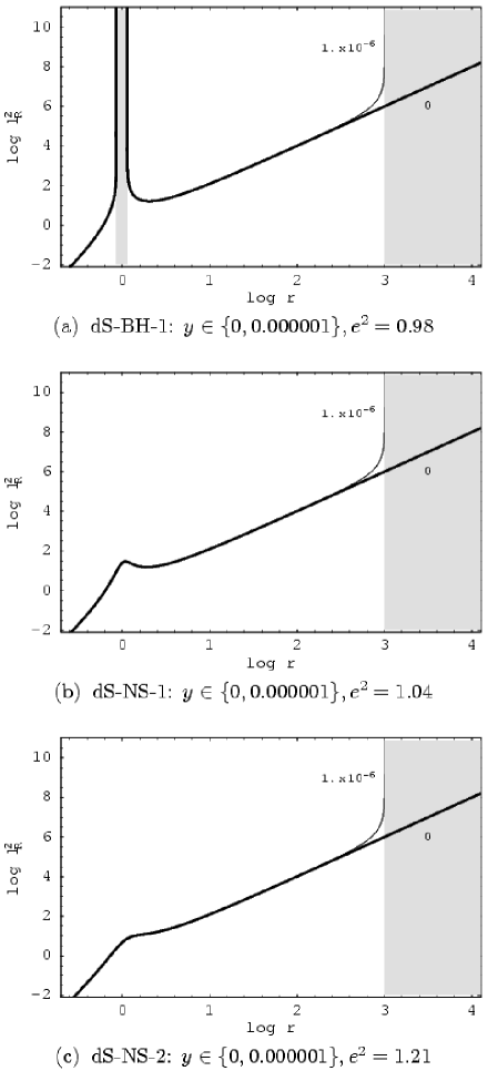
Figure 6: The effective potential $\ell^{2}_{\mathrm{R}}(r;e,y)$ of the photon geodetical motion in the asymptotically de Sitter spacetimes. There are three qualitatively different types of the behavior of $\ell^{2}_{\mathrm{R}}$, according to the value of the charge parameter $e^{2}$, as illustrated in the cases (a) through (c). The dynamic regions of the spacetimes, where $\ell^{2}_{\mathrm{R}}$ is not well defined, are shaded. For comparison, the effective potential is given for the corresponding Reissner–Nordström spacetimes with $y=0$ (bold lines). Clearly, the difference occurs at the region near the cosmological horizon. Loci of the photon circular orbits (cases (a) and (b)) are independent of $y$.

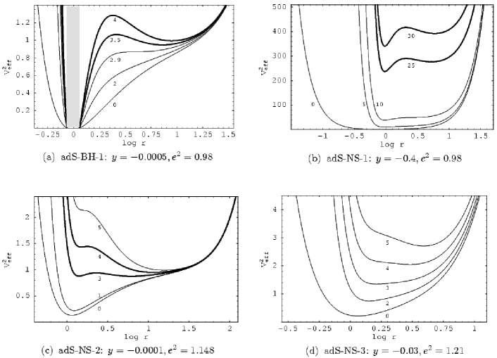
Figure 7: The effective potential $V^{2}_{\mathrm{eff}}(r;e,y,L)$ of the test-particle geodetical motion in the asymptotically anti-de Sitter spacetimes. There are four qualitatively different types of the behavior of $V^{2}_{\mathrm{eff}}$ subsequently illustrated in the cases (a) through (d). The curves giving the effective potential are labeled by the values of the particle’s angular momentum $L$. In the black-hole spacetimes, only one type of the behavior of $V^{2}_{\mathrm{eff}}$ is possible; it is shown in the case a), where the dynamic region of the spacetime is shaded. Note that in all of types of the behavior of $V^{2}_{\mathrm{eff}}$, there is a minimum of the effective potential for $L\to\infty$, located at $r\to\infty$, with energy of the circular orbit $E_{\mathrm{c}}\to\infty$. Therefore, in the limit of ultrarelativistic particles a photon circular geodesic appears for $r\to\infty$.

Distribution of these types of the Reissner–Nordström–(anti-)de Sitter spacetimes in the parameter space $e^{2}$-$y$ is shown in Fig. 3. According to the presented classification of the spacetimes, seven (four) types of the behavior of the effective potential of the geodetical motion in the asymptotically de Sitter (anti-de Sitter) spacetimes are shown in Fig. 5 (Fig. 7). Properties of the effective potential can be summarized in the following way, separating the cases of the asymptotically de Sitter ($y>0$), and anti-de Sitter ($y<0$) spacetimes.

A1 Reissner–Nordström–de Sitter black-hole spacetimes

There are two types of the black-hole spacetimes (dS-BH-1 and 2) with different behavior of the effective potential $V^{2}_{\mathrm{eff}}(r;L,e,y)$ of the test particle motion (see Fig. 5a,b) In both cases, the effective potential has no local extrema at $r<r_{\mathrm{b}-}$ for any value of the specific angular momentum $L$ of the particles. Local minima of $V^{2}_{\mathrm{eff}}$, corresponding to stable circular orbits, exist for a limited range of $L$ in the dS-BH-1 type only. In both dS-BH-1 and 2 spacetimes, there are maxima of $V^{2}_{\mathrm{eff}}$ at $r>r_{\mathrm{b}+}$. In dS-BH-1 spacetimes there are even two maxima of $V^{2}_{\mathrm{eff}}$ in the range of $L$ allowing the stable circular orbits. One maximum exists for any $L\geq 0$ in both dS-BH-1 and 2 spacetimes. In the limit of $L\to\infty$, its loci $r\to r_{\mathrm{ph}+}$. Therefore, it corresponds to the photon circular orbit.

The generalized effective potential of the photon motion $\ell^{2}_{\mathrm{R}}(r;e,y)$ has the same character for all black-hole spacetimes (see Fig. 6a). It has always a minimum at $r=r_{\mathrm{ph}}>r_{\mathrm{b}+}$, corresponding to the photon circular orbit. It diverges at all the event horizons, and has no local extrema at $r<r_{\mathrm{b}-}$.

We can conclude that both $V^{2}_{\mathrm{eff}}(r;L,e,y)$ and $\ell^{2}_{\mathrm{R}}(r;e,y)$ have the same character as in the case of Schwarzschild–de Sitter black holes. The differences with respect to the Reissner–Nordström black holes are given by the differences of the asymptotic character of flat and de Sitter spacetimes. Especially, there are no Reissner–Nordström black holes admitting unstable circular geodesics only, as happens in the case of dS-BH-2 spacetimes.

A2 Reissner–Nordström–de Sitter naked-singularity spacetimes

There are five types of the naked-singularity spacetimes (dS-NS-1 through 5), with different behavior of $V^{2}_{\mathrm{eff}}(r;e,y,L)$ (see Fig. 5c–g). In the spacetimes dS-NS-1 and 2, the effective potential has a local minimum and a local maximum for all $L\geq 0$. In the limit of $L\to\infty$, loci of the minimum $r\to r_{\mathrm{ph}-}$, where $V^{2}_{\mathrm{eff}}$ diverges, and loci of the maximum $r\to r_{\mathrm{ph}+}$, where $V^{2}_{\mathrm{eff}}$ diverges, too. At $r=r_{\mathrm{ph}-}$ ($r=r_{\mathrm{ph}+}$), the stable (unstable) photon circular orbit is located. In the dS-NS-1 spacetimes, an additional minimum and maximum of $V^{2}_{\mathrm{eff}}$ occurs for a limited range of $L>0$. Therefore, two separated regions of both stable and unstable circular geodesics exist in these spacetimes. In the spacetimes dS-NS-3 and 4, the local minima and maxima exist for a range of $L$ limited from above ($0\leq L<L_{\mathrm{u}1}$), and in the dS-NS-3 spacetimes, there is an additional minimum and maximum for $L$ in the range ($L_{\mathrm{d}}<L<L_{\mathrm{u}2}$), with $L_{\mathrm{u}2}<L_{\mathrm{u}1}$. It is important that in all of the naked—singularity spacetimes dS-NS-1 through 4, there is a stationary particle (a ‘circular orbit’ with $L=0$) at an inner, stable static radius, and an outer, unstable static radius. An exception is represented by the spacetimes dS-NS-5 with $V^{2}_{\mathrm{eff}}$ having no local extrema.

There are two types of the behavior of the function $\ell^{2}_{\mathrm{R}}(r;e,y)$ determining photon motion. For $1<e^{2}<9/8$, $\ell^{2}_{\mathrm{R}}$ has an inner local maximum at $r=r_{\mathrm{ph}-}$ (stable circular photon orbit) and an outer local minimum at $r=r_{\mathrm{ph}+}$ (unstable photon circular orbit)—see Fig. 6b. For $e^{2}>9/8$, there are no local extrema of $\ell^{2}_{\mathrm{R}}$ and no photon circular orbits—see Fig. 6c.

We can conclude that for the photon motion, the new feature of $\ell^{2}_{\mathrm{R}}(r;e,y)$ in comparison with the case of Reissner–Nordström naked singularities is given by the asymptotic behavior of $\ell^{2}_{\mathrm{R}}$ only. On the other hand, for test-particle motion, the differences are given by the asymptotic behavior in all of the dS-NS-1 through 4 spacetimes, but there are also new features caused by the interplay of the spacetime parameters $e$ and $y$. In dS-NS-2 through 4 spacetimes, the inner region of stable orbits is followed by an outer region of unstable orbits—such a behavior is impossible in the field of Reissner–Nordström naked singularities. Comparison with the Schwarzschild–de Sitter naked-singularity spacetimes is meaningless as these spacetimes have no static regions.

B1 Reissner–Nordström–anti-de Sitter black-hole spacetimes

There is only one type of black-hole spacetimes (AdS-BH-1) with respect to behavior of both $V^{2}_{\mathrm{eff}}(r;e,y,L)$ and $\ell^{2}_{\mathrm{R}}(r;e,y)$. $V^{2}_{\mathrm{eff}}$ has a local maximum (unstable circular orbit) and a local minimum (stable circular orbit) for the specific angular momentum $L>L_{\mathrm{d}}>0$. If $L\to\infty$, loci of the minimum $r\to r_{\mathrm{ph}+}$ and $V^{2}_{\mathrm{eff}}\to\infty$, while loci of the maximum $r\to\infty$ and $V^{2}_{\mathrm{eff}}\to\infty$—see Fig. 7a. At $r=r_{\mathrm{ph}+}$, an unstable photon circular orbit is located; at $r\to\infty$ a stable circular photon orbit is located, in the sense defined below.

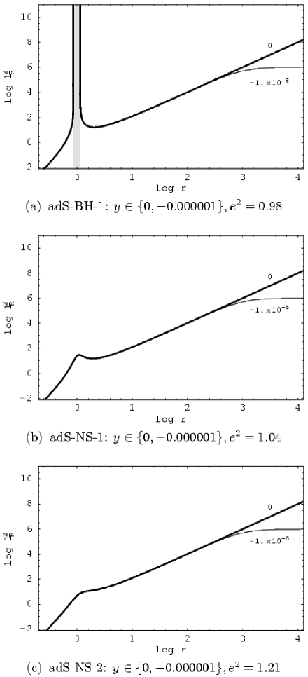
Figure 8: The effective potential $\ell^{2}_{\mathrm{R}}(r;e,y)$ of the photon geodetical motion in the asymptotically anti-de Sitter spacetimes. There are three qualitatively different types of $\ell^{2}_{\mathrm{R}}$ according to the value of the charge parameter $e^{2}$, illustrated in the cases (a) through (c). The dynamic region of the black-hole spacetime (case (a)) is shaded. For comparison, $\ell^{2}_{\mathrm{R}}(r;e,y=0)$ of the corresponding Reissner–Nordström spacetimes (drawn by bold solid lines) are included in all of the considered cases. Clearly, in all of the cases (a) through (c), the qualitative differences are caused by the attractive cosmological constant at large radii. Loci of the photon circular orbits, given by local extrema of $\ell^{2}_{\mathrm{R}}$, are independent of $y$.

The generalized effective potential of the photon motion (see Fig. 8a) has a local minimum at $r=r_{\mathrm{ph}+}$ for all values of $e^{2}<1$. Further, there is

$$\ell^{2}_{\mathrm{R}}(r\to\infty;e,y)\to(-y)^{-1/2}.$$ (38)

Therefore, in this sense, a stable circular photon orbit can exist for $r\to\infty$. It can be considered as a limit of stable circular orbits of ultrarelativistic particles at radii $r\to\infty$. The function $\ell^{2}_{\mathrm{R}}(r;e,y)$ diverges at both event horizons, and has no local extrema under the inner horizon $r_{\mathrm{b}-}$.

Both $V^{2}_{\mathrm{eff}}(r;e,y,L)$ and $\ell^{2}_{\mathrm{R}}(r;e,y)$ have the same character as in the case of Schwarzschild–anti-de Sitter black holes. Differences in comparison with the Reissner–Nordström black hole are given by the asymptotic behavior of $V^{2}_{\mathrm{eff}}$ and $\ell^{2}_{\mathrm{R}}$ only.

B2 Reissner–Nordström–anti-de Sitter naked-singularity spacetimes

There are three types of the naked-singularity spacetimes (AdS-NS-1 through 3) with different behavior of $V^{2}_{\mathrm{eff}}(r;e,y,L)$—see Fig. 7b–d. In all of these spacetimes, there is a local minimum of $V^{2}_{\mathrm{eff}}$ for $L$ from the interval $0\leq L<\infty$. If $L=0$, the minimum corresponds to the stable static radius where a test particle can be in a stable equilibrium position. If $L>0$, the minimum corresponds to a stable circular orbit. For $L\to\infty$, its loci $r\to\infty$ which corresponds to a stable photon circular orbit in the limit of stable circular orbits of ultrarelativistic particles, with impact parameter given by Eq. (38); this is the same situation as in the case of black-hole spacetimes AdS-BH-1.

In the spacetimes AdS-NS-1, there is additionally a local minimum, and a local maximum, corresponding to stable and unstable circular orbits, if $0<L_{\mathrm{d}}<L<\infty$. In the limit of $L\to\infty$ the local minimum diverges ($V^{2}_{\mathrm{eff}}\to\infty$) at $r\to r_{\mathrm{ph}-}$, corresponding to a stable circular photon orbit, while the local maximum diverges at $r\to r_{\mathrm{ph}+}$, corresponding to an unstable circular photon orbit. In the spacetimes AdS-NS-2, the additional local minima and maxima are allowed in a limited range of $L_{\mathrm{d}}<L<L_{\mathrm{u}}$, while they are not allowed at all in the spacetimes AdS-NS-3.

Similarly to the case of Reissner–Nordström–de Sitter naked singularity spacetimes, there are two types of the behavior of $\ell^{2}_{\mathrm{R}}(r;e,y)$ governing photon motion. For $1<e^{2}<9/8$ (see Fig. 8b), there is an inner local maximum at $r=r_{\mathrm{ph}-}$ (stable circular photon orbit), and an outer local minimum at $r=r_{\mathrm{ph}+}$ (unstable circular photon orbit). For $e^{2}>9/8$ (Fig. 8c), $\ell^{2}_{\mathrm{R}}(r;e,y)$ has no local extrema. In both cases, the asymptotic behavior of $\ell^{2}_{\mathrm{R}}(r;e,y)$ is given by Eq. (38), as in the black-hole case.

Comparing behavior of $V^{2}_{\mathrm{eff}}(r;e,y,L)$ and $\ell^{2}_{\mathrm{R}}(r;e,y)$ with the case of Reissner–Nordström naked singularities, we have to emphasize the differences of the behavior in the asymptotic region of $r\to\infty$. There is no other difference caused by the interplay of the charge parameter $e$, and the attractive cosmological parameter $y<0$.

Distribution of all eleven types of the Reissner–Nordström–(anti-)de Sitter spacetimes in the parameter space $e^{2}$-$y$ is given in Fig. 3.

4 Photon escape cones

We shall discuss the influence of both the repulsive and attractive cosmological constant on the character of photon escape cones related to the family of static observers. Although related to the local observers, the photon escape cones reflect global properties of the spacetimes under consideration. We shall consider regions above the outer black-hole horizon and complete naked-singularity spacetimes.

The orthonormal tetrad of vectors carried by the static observers is

$$\hbox{\boldmath$\textstyle e$}_{(t)} = \left(1-\frac{2}{r}+\frac{e^{2}}{r^{2}}-yr^{2}\right)^{1/2}\frac{\partial}{\partial t},$$ (39)

$$\hbox{\boldmath$\textstyle e$}_{(r)} = \left(1-\frac{2}{r}+\frac{e^{2}}{r^{2}}-yr^{2}\right)^{-1/2}\frac{\partial}{\partial r},$$ (40)

$$\hbox{\boldmath$\textstyle e$}_{(\theta)} = \frac{1}{r}\frac{\partial}{\partial\theta},$$ (41)

$$\hbox{\boldmath$\textstyle e$}_{(\phi)} = \frac{1}{r\sin\theta}\frac{\partial}{\partial\phi}.$$ (42)

The components of the four-momentum of a photon as measured by a static observer are given by

$$p_{(\alpha)}=p_{\mu}e^{\mu}_{(\alpha)}.$$ (43)

Using relations

$$p^{(t)}=-p_{(t)},\quad p^{(\phi)}=p_{(\phi)},$$ (44)

we can give the directional angle $\psi$ of the photon, i.e., the angle measured by the observer relative to its outward radial direction, in the form

$$\sin\psi = \frac{p^{(\phi)}}{p^{(t)}}=\left(1-\frac{2}{r}+\frac{e^{2}}{r^{2}}-yr^{2}\right)^{1/2}\frac{\ell}{r},$$ (45)

$$\cos\psi = \frac{p^{(r)}}{p^{(t)}}=\pm\left[1-\left(1-\frac{2}{r}+\frac{e^{2}}{r^{2}}-yr^{2}\right)\frac{\ell^{2}}{r^{2}}\right]^{1/2}.$$ (46)

The photon escape cones can be determined by using the ‘effective potential’ $\ell^{2}_{\mathrm{R}}(r;y,e)$ of the photon motion. In establishing the directional angle $\psi_{\mathrm{c}}$ of a marginally escaping photon, the impact parameter $\ell_{\mathrm{c}}$ of the unstable circular photon orbit plays the crucial role for static observers located both under and above the unstable circular photon orbit at $r=r_{\mathrm{ph}+}(e)$; for simplicity we consider only positive values of $\ell_{\mathrm{c}}$ because the cone is symmetric about the radial direction. In appropriately chosen regions of the naked-singularity spacetimes admitting two circular photon orbits, there are directional angles corresponding to bound photons. The bound photons are concentrated around the stable circular photon orbit at $r_{\mathrm{ph}-}(e)<r_{\mathrm{ph}+}(e)$.

In the black-hole backgrounds (above their outer horizon), the photon directional angles can be separated into the escape cones, and the complementary captured cones. In the naked-singularity backgrounds admitting two circular photon orbits, there is a region extending under the radius of the unstable photon circular orbit and crossing the radius of the stable photon circular orbit, where the escape cone is complemented by the cone corresponding to directions of bound photons. This bound cone is concentrated about the direction corresponding to the stable photon circular orbit.

At $r=r_{\mathrm{ph}+}(e)$, the escape angle is determined by

$$\psi_{\mathrm{c}}(r=r_{\mathrm{ph}+},y,e)=\frac{\pi}{2},$$ (47)

independently of $y$. At $r\neq r_{\mathrm{ph}+}(e)$, escaping directional angles are determined by the formulae

$$\sin\psi_{\mathrm{c}}(r;y,e) = \left(1-\frac{2}{r}+\frac{e^{2}}{r^{2}}-yr^{2}\right)^{1/2}\frac{\ell_{\mathrm{c}+}(y,e)}{r},$$ (48)

$$\cos\psi_{\mathrm{c}}(r;y,e) = \pm\left[1-\left(1-\frac{2}{r}+\frac{e^{2}}{r^{2}}-yr^{2}\right)\frac{\ell^{2}_{\mathrm{c}+}(y,e)}{r^{2}}\right]^{1/2},$$ (49)

where $\ell_{\mathrm{c}+}(y,e)$ is given by Eq. (25). For $r<r_{\mathrm{ph}+}$, the marginally escaping photon is radially outwards directed ($p^{(r)}>0$ and $\cos\psi_{\mathrm{c}}$ is taken with ‘$+$’ sign), for $r>r_{\mathrm{ph}+}$, it is inwards directed ($p^{(r)}<0$ and $\cos\psi_{\mathrm{c}}$ is taken with ‘$-$’ sign). If $e^{2}=0$, and $y\neq 0$, we arrive at the relations for the escape directional angles at the Schwarzschild–(anti-)de Sitter spacetimes [14]

$$\sin\psi_{\mathrm{c}}(r;y) = \left[\frac{27(r-2-yr^{3})}{r^{3}(1-27y)}\right]^{1/2},$$ (50)

$$\cos\psi_{\mathrm{c}}(r;y) = \pm\left[\frac{r^{3}-27r+54}{r^{3}(1-27y)}\right]^{1/2}.$$ (51)

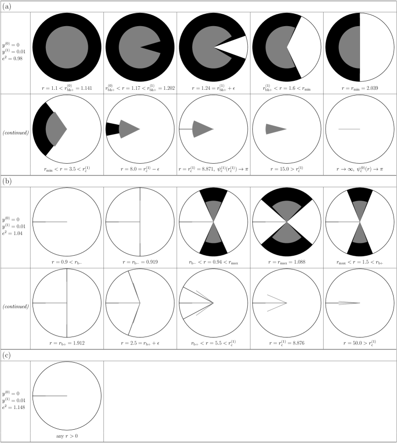
Figure 9: The photon escape cones in the asymptotically de Sitter spacetimes. They are constructed at a representative sequence of radii. There are three qualitatively different types of the character of the escape cones, in accord with behaviour of $\ell^{2}_{\mathrm{R}}(r;e,y)$ (cf.  Fig. 6). Complementary to the escape cones are the capture cones in the black-hole spacetimes (case (a)), and the bound cones in the naked-singularity spacetimes (case (b)). Because of the central symmetry, we show central sections of the cones. The inward-directed radial direction is represented by the horizontal, left-oriented line from the centre. The captured cones (case (a)) and bound cones (case (b)) are dark shaded. For comparison, we consider the escape and the complementary cones in the corresponding Reissner–Nordström spacetimes; in this case the captured or bound cones are gray shaded. Notice that at all radii in the naked-singularity spacetimes, the captured photons correspond to a singular case of inward radial direction.

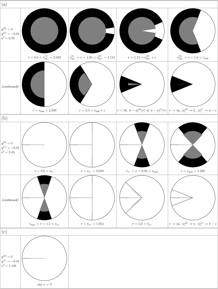
Figure 10: The photon escape cones in the asymptotically anti-de Sitter spacetimes. Constructed at representatively selected radii. There are three qualitatively different types of the behaviour of the escape cones, in accord with behaviour of $\ell^{2}_{\mathrm{R}}(r;e,y)$ (cf. Fig. 8). The cones are constructed in the same way as for the asymptotically de Sitter spacetimes (see the caption of Fig. 9). Notice that due to the influence of the attractive cosmological constant, the capture cones at the black-hole spacetimes remain nonzero in the limit of $r\to\infty$, and their extension is determined by the cosmological parameter $y$.

Using the relations for the escaping directional angles, the behavior of the escape cones is established and illustrated in Fig. 9 (Fig. 10) for asymptotically de Sitter (anti-de Sitter) spacetimes. For comparison, the escape cones corresponding to the Reissner–Nordström spacetimes with the same parameter $e$ and $y=0$ are included. The results are summarized in the following way.

A1 The Reissner–Nordström–de Sitter black-hole spacetimes

The behavior of the escape cones is presented in Fig. 9a. At a fixed (and allowed) $r<r_{\mathrm{ph}+}$, the escape cone of the Reissner–Nordström black hole is the widest one, and it gets smaller with $y$ growing. On the other hand, at a fixed (and allowed) $r>r_{\mathrm{ph}+}$, the Reissner–Nordström escape cone is smallest one. Of course, the complementary Reissner–Nordström photon capture cone is the widest one at $r>r_{\mathrm{ph}+}$. Close to the cosmological horizon, the Reissner–Nordström–de Sitter capture cone gets to be strongly narrower than the Reissner–Nordström cone.

A2 The Reissner–Nordström–de Sitter naked-singularity spacetimes

The behavior of the escape and bound cones is presented in Fig. 9b. In the spacetimes with $e^{2}<9/8$, the bound cones are restricted to some region under the outer, unstable circular photon orbit at $r_{\mathrm{ph}+}$. They are concentrated around the inner, stable circular photon orbit at $r_{\mathrm{ph}-}$, where the bound cones are most extended. At $r>r_{\mathrm{ph}+}$, there are singular directions corresponding to bound photons, radiated at the $\psi_{\mathrm{c}}$ directional angle in the inward direction, which wind up at the unstable photon circular orbit. For $r\to r_{\mathrm{c}}$, there is $\psi_{\mathrm{c}}\to\pi$. For the spacetimes with $e^{2}>9/8$, there are only escaping photons at all radii up to the cosmological horizon (Fig. 9c). In both types of the naked-singularity spacetimes, at all radii $r<r_{\mathrm{c}}$ the captured cones degenerate to the singular case of photons with $l=0$ and $\psi=\pi$, terminated at the physical singularity ($r=0$).

B1 The Reissner–Nordström–anti-de Sitter black-hole spacetimes

The behavior of the escape (capture) cones is presented in Fig. 10a. At a fixed (and allowed) $r<r_{\mathrm{ph}+}$, the escape cone of the Reissner–Nordström spacetime is the narrowest one; if gets wider with $y$ descending. At a fixed $r>r_{\mathrm{ph}+}$, the Reissner–Nordström escape cone becomes wider than the cones with $y<0$. The complementary photon capture cone of the Reissner–Nordström spacetime lies inside the capture cones of the spacetimes with $y<0$. Asymptotically ($r\to\infty$), the Reissner–Nordström capture cone degenerates into the inward radial direction, while the Reissner–Nordström–anti-de Sitter cone converges to a cone with a nonzero opening angle equal to

$$\psi_{\mathrm{c}}(r\to\infty,y<0,e)\sim[\sin^{-1}\left(\ell_{\mathrm{c}+}(y,e)\right)(-y)^{1/2}].$$ (52)

Now, the asymptotic behavior of the capture cones is strongly influenced by the asymptotic character of these spacetimes.

B2 The Reissner–Nordström–anti-de Sitter naked-singularity spacetimes

For the spacetimes with $e^{2}<9/8$, the behavior of the escape and bound cones is presented in Fig. 10b. The bound cones are widest for the Reissner–Nordström naked singularities. At $r>r_{\mathrm{ph}+}$, there is again the singular direction corresponding to bound photons which wind up on the unstable photon orbit. However, for $r\to\infty$, there is $\pi-\psi_{\mathrm{c}}\neq 0$. The angle $\psi_{\mathrm{c}}$ is given by Eq. (52). If $e^{2}>9/8$, all photons escape from any $r>0$. In both types of the naked-singularity spacetimes the capture cones shrink at all radii $r>0$ to the singular case of photons radiated radially inwards with $l=0$ and $\psi=\pi$ that terminate at the singularity at $r=0$.

5 Embedding of the ordinary geometry

Curvature of the static parts of the black-hole and naked-singularity Reissner–Nordström spacetimes with a nonzero cosmological constant can be represented in highly illustrative way by embedding diagrams. Comparison of these embedding diagrams with those constructed for the pure Reissner–Nordström or Schwarzschild spacetimes [9, 12] gives an intuitive insight into the change of the character of the spacetime caused by the cosmological constant and its interplay with the charge parameter of the spacetime.

The existence of the field of the time Killing vector $\partial/\partial t$ enables us to define a privileged notion of space using the hypersurfaces of $t=\mathrm{const}$. We shall use the induced metric on these hypersurfaces (i.e., the space components of the metric tensor $g_{ik}$)—we call it ordinary space. Geometry of all the central planes of the ordinary geometry is the same as those of the equatorial plane ($\theta=\pi/2=\mathrm{const}$) as a consequence of the central symmetry of the spherically symmetric spacetimes. Therefore, the embedding diagrams will be constructed for the simplest case of the equatorial plane.

We shall embed the surface described by the line element

$$\mathrm{d}\ell^{2}_{\mathrm{(RNdS)}}=\left(1-\frac{2}{r}+\frac{e^{2}}{r^{2}}-yr^{2}\right)^{-1}\mathrm{d}r^{2}+r^{2}\,\mathrm{d}\phi^{2}$$ (53)

into the flat Euclidean three-dimensional space with line element expressed in the standard cylindrical coordinates ($\rho,z,\phi$) in the form

$$\mathrm{d}\sigma^{2}=\mathrm{d}\rho^{2}+\rho^{2}\,\mathrm{d}\phi^{2}+\mathrm{d}z^{2}.$$ (54)

The embedding is represented by the rotationally symmetric surface $z=z(\rho)$ in the Euclidean space. Its geometry has to be isometric with the geometry of the equatorial plane described by (53). Thus we have to identify the line element

$$\mathrm{d}\ell^{2}_{\mathrm{(E)}}=\left[1+\left(\frac{\mathrm{d}z}{\mathrm{d}\rho}\right)^{2}\right]\mathrm{d}\rho^{2}+\rho^{2}\,\mathrm{d}\phi^{2},$$ (55)

with the line element (53). We can identify both the azimuthal and radial coordinates ($r\equiv\rho$). The embedding diagram can then be given by the embedding formula $z=z(r)$, which can be obtained by integrating the relation

$$\frac{\mathrm{d}z}{\mathrm{d}r}=\pm\left(\frac{yr^{4}+2r-e^{2}}{-yr^{4}+r^{2}-2r+e^{2}}\right)^{1/2}.$$ (56)

The sign in this formula is irrelevant, leading to isometric surfaces.

Since the embedding diagrams have to be constructed at the static regions, where denominator at the right hand side of (56) is nonzero, the limits of embeddability are given by the condition

$$yr^{4}+2r-e^{2}\geq 0,$$ (57)

which can be rewritten in the form

$$y\geq y_{\mathrm{e(ord)}}(r;e)\equiv\frac{-2r+e^{2}}{r^{4}}.$$ (58)

The asymptotic behavior of the function $y_{\mathrm{e(ord)}}(r;e)$ determining limit of embeddability of the ordinary space is given by relations

$$y_{\mathrm{e(ord)}}(r\to 0,e)\to+\infty,\quad y_{\mathrm{e(ord)}}(r\to\infty,e)\to 0.$$ (59)

The zero point of the function $y_{\mathrm{e(ord)}}(r;e)$ is given by

$$e^{2}=e^{2}_{\mathrm{z(e(ord))}}\equiv 2r,$$ (60)

its local minimum is located at

$$e^{2}=e^{2}_{\mathrm{min(e(ord))}}=\textstyle\frac{3}{2}r,$$ (61)

where

$$y_{\mathrm{e(ord)(min)}}(e)=-\frac{27}{16e^{6}}.$$ (62)

The functions (60) and (61) are illustrated in Fig. 11. The function (62) is illustrated in Fig. 12.

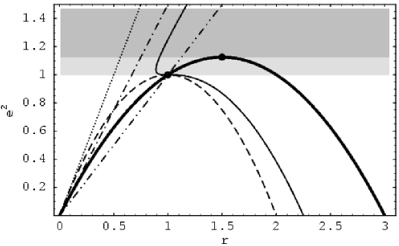
Figure 11: The characteristic functions governing properties of the embedding diagrams of both the ordinary space and the optical reference geometry associated with the Reissner–Nordström–(anti-)de Sitter spacetimes. The characteristic function $e^{2}_{\mathrm{e(h)}}(r)$ (represented by the bold solid line) governs the local extrema of the function $y_{\mathrm{h}}(r;e)$ determining the event horizons of the spacetimes. Its local maximum is located at the point $(3/2,9/8)$. The function $e^{2}_{\mathrm{z(h)}}(r)$ (represented by the dashed line) governs the zero points of $y_{\mathrm{h}}(r;e)$, i.e., the event horizons of the Reissner–Nordström black holes. The function $e^{2}_{\mathrm{z(e(ord))}}(r)$ (dotted line) represents zero points and the function $e^{2}_{\mathrm{min(e(ord))}}(r)$ (dash-dotted line) represents the local minimum of the function $y_{\mathrm{e(ord)}}(r;e)$ governing the limits of embeddability of the ordinary space. The function $e^{2}_{\mathrm{z(e(opt))}}(r)$ (light solid line) determines the zero point of the function $y_{\mathrm{e(opt)}}(r;e)$ governing the limits of embeddability of the optical space. The local extrema of $y_{\mathrm{e(opt)}}(r;e)$ are given by the function $e^{2}=r$ (dash-two-dotted line), and by the function $e^{2}_{\mathrm{e(h)}}(r)$ (bold solid line) governing also the radii of photon circular geodesics that are independent of the cosmological parameter $y$, coinciding with the extreme points of $y_{\mathrm{h}}(r;e)$. The extrema of the functions $e^{2}_{\mathrm{e(h)}}(r)$ and $e^{2}_{\mathrm{z(h)}}(r)$ (depicted by the bold dots) divide the nonnegative region of the charge parameter $e^{2}$ into three subintervals emphasized by increasing gray level, each of them implying different behavior of the functions $y_{\mathrm{h}}(r;e)$, $y_{\mathrm{e(ord)}}(r;e)$, $y_{\mathrm{e(opt)}}(r;e)$.

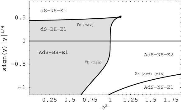
Figure 12: The classification of the Reissner–Nordström–(anti-)de Sitter spacetimes according to the properties of the embedding diagrams of their ordinary space geometry. The functions $y_{\mathrm{h(min)}}(e)$ and $y_{\mathrm{h(max)}}(e)$ limit the black-hole spacetimes (shaded region) in the parameter space $e^{2}$-$y$. Outside that region, merely naked-singularity spacetimes exist. The function $y_{\mathrm{e(ord)(min)}}(e)$ separates the spacetimes AdS-NS-E1 having no space region embeddable into the Euclidean space.

The regions of embeddability are given by the condition

$$y_{\mathrm{e(ord)}}(r;e)<y<y_{\mathrm{h}}(r;e).$$ (63)

The embeddings of the Schwarzschild–(anti-)de Sitter spacetimes are discussed in Ref. [14] and will not be repeated here. There are three qualitatively different types of the behavior of the functions $y_{\mathrm{e(ord)}}(r;e)$ and $y_{\mathrm{h}}(r;e)$ in the Reissner–Nordström spacetimes with $\Lambda\neq 0$: (a) $0<e^{2}\leq 1$, (b) $1<e^{2}\leq 9/8$, (c) $e^{2}>9/8$. They are illustrated in Fig. 13.

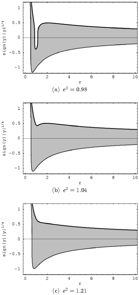
Figure 13: Embeddability of the ordinary space geometry of the Reissner–Nordström–(anti-)de Sitter spacetimes. According to values of the charge parameter $e^{2}$, there are three qualitatively different types (cases (a) through (c)) of the behaviour of the functions $y_{\mathrm{h}}(r;e)$ (bold solid lines), and $y_{\mathrm{e(ord)}}(r;e)$ (thin solid lines) determining regions of embeddability. The regions of embeddability are shaded.

Analysis of these functions enables an appropriate classification of the spacetimes according to the properties of the embedding diagrams of the ordinary space. There are five types of the Reissner–Nordström–(anti-)de Sitter spacetimes with qualitatively different behavior of the embedding diagrams as directly follows from Fig. 13.

In the parameter space $e^{2}$-$y$, distribution of the five different types of the Reissner–Nordström–(anti-)de Sitter spacetimes according to properties of the embedding diagrams of their ordinary (space) geometry is quite simple, as it follows distribution of black holes and naked singularities with $y>0$ and $y<0$ . There is the only exception represented by asymptotically anti-de Sitter naked singularities which are separated into two parts (AdS-NS-1 and 2), as shown in Fig. 12.

We briefly summarize the properties of the embedding diagrams.

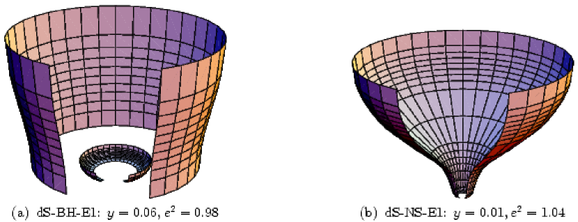
Figure 14: Typical embedding diagrams of the ordinary space geometry of the asymptotically de Sitter spacetimes. There is one type of the embedding diagrams for black holes (case (a)), and the other one for naked singularities (case b). In both cases there is a funnel near the cosmological horizon. For black holes, the embedding can be extended down to the outer horizon and up to the inner horizon. For both black holes and naked singularities, the embedding cannot be extended down to the singularity at $r=0$.

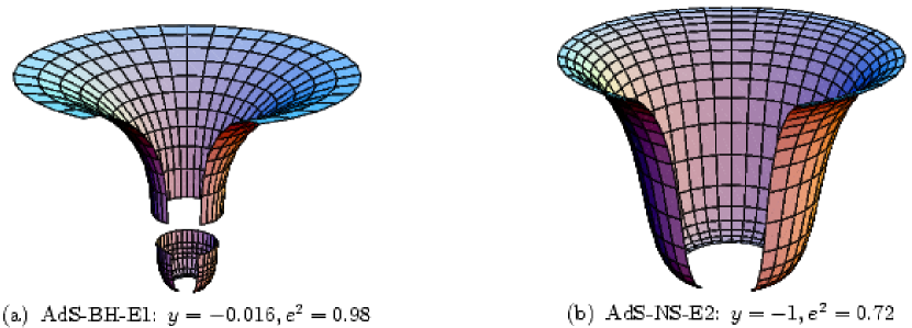
Figure 15: Typical embedding diagrams of the ordinary space geometry of the asymptotically anti-de Sitter spacetimes. There is one type of the diagram for black holes (case (a)), and the other one for naked singularities (case (b)). In both cases, the embedding diagrams cannot be extended up to infinity. Note that for some of the naked-singularity spacetimes (type AdS-NS-1) no region is embeddable into the Euclidean space.

A1 Reissner–Nordström–de Sitter black-hole spacetimes

The embedding diagrams have the same character for all allowed values of $e$ and $y$; following the method introduced in the discussion of the effective potential of the geodetical motion, we denote the type as dS-BH-E1. A typical embedding is given in Fig. 14a. The ordinary space between the outer black-hole horizon $r_{\mathrm{b}+}$ and the cosmological horizon $r_{\mathrm{c}}$ can always be embedded—the embedding resembles a funnel having a throat near both the horizons. This is the same behavior as in the case of Schwarzschild–de Sitter black holes (for details see Ref. [14]). On the other hand, embeddability of the space under the black-hole inner horizon is limited from below.

A2 Reissner–Nordström–de Sitter naked-singularity spacetimes

The embedding diagrams have the same character for all allowed values of $e$, and $y$; we denote the type as dS-NS-E1, and we show a typical embedding in Fig. 14b. The ordinary space is embeddable from a lower bound given by the function $y_{\mathrm{e(ord)}}(r;e)$ up to the cosmological horizon. The embedding diagram has a throat near the cosmological horizon.

B1 Reissner–Nordström–anti-de Sitter black-hole spacetimes

The embedding diagrams are of the same nature for all black holes; we denote the type as AdS-BH-E1. A typical embedding diagram is shown in Fig. 15a. The embedding consists of two regions, the inner one approaches the inner horizon being limited from below. The outer region approaches the outer horizon being limited from above.

B2 Reissner–Nordström–anti-de Sitter naked-singularity spacetimes

There are two types of naked singularities with respect to embeddability of the ordinary space. The type AdS-NS-E1 has no region that could be embedded into Euclidean space. The type AdS-NS-E2 has a region that can be embedded, but it is limited both from below and from above; a typical embedding is shown in Fig. 15b.

6 Optical reference geometry and the inertial forces

The optical reference geometry enables us to introduce the concept of gravitational and inertial forces in the framework of general relativity in a natural way [11, 19, 20, 21, 22, 23, 24, 25, 26]. In accord with the spirit of general relativity, alternative approaches to the concept of inertial forces are possible [27, 28], however, the optical geometry provides a description of relativistic dynamics in accord with Newtonian intuition. The optical geometry results from an appropriate conformal ($3+1$) splitting, reflecting certain hidden properties of the spacetime under consideration through its geodetical structure. The geodesics of the optical geometry related to static spacetimes coincide with trajectories of light, thus being ‘optically straight’ [10, 29]. Moreover, the geodesics are ‘dynamically straight,’ because test particles moving along them are kept by a velocity-independent force [11], and they are also ‘inertially straight,’ because gyroscopes carried along them do not precess along the direction of the motion [11, 20].

The notions of the optical geometry and the related gravitational and inertial forces are convenient for spacetimes with symmetries, particularly for stationary (static) and axisymmetric (spherically symmetric) ones. However, they can be introduced for a general spacetime lacking any symmetry [20]. Assuming a hypersurface globally orthogonal to a timelike unit vector field $n^{\kappa}$ and a scalar function $\Phi$ satisfying the conditions

$$n_{[\kappa}\nabla\!_{\lambda}n_{\mu]} = 0,$$ (64)

$$n^{\kappa}n_{\kappa} = 1,$$ (65)

$$\dot{a}_{\lambda} = n^{\kappa}\nabla\!_{\kappa}n_{\lambda}=\nabla\!_{\lambda}\Phi,$$ (66)

the four-velocity $u^{\kappa}$ of a test particle of rest mass $m$ can be uniquely decomposed as

$$u^{\kappa}=\gamma\left(n^{\kappa}+v\tau^{\kappa}\right),$$ (67)

where $\tau^{\kappa}$ is a unit vector orthogonal to $n^{\kappa}$, $v$ is the speed and $\gamma=(1-v^{2})^{-1/2}$ is the Lorentz factor. According to Abramowicz, Nurowski and Wex [19] so called ordinary projected geometry (three-space orthogonal to $n^{\kappa}$) can be introduced by

$$h_{\kappa\lambda}=g_{\kappa\lambda}+n_{\kappa}n_{\lambda}$$ (68)

and the optical geometry by conformal rescaling

$$\tilde{h}_{\kappa\lambda}=e^{-2\Phi}\left(g_{\kappa\lambda}+n_{\kappa}n_{\lambda}\right).$$ (69)

Then the projection of the four-acceleration $a^{\bot}_{\kappa}=h^{\lambda}_{\kappa}u^{\mu}\nabla\!_{\mu}u_{\lambda}$ can be uniquely decomposed into terms proportional to zeroth, first and second powers of $v$, respectively and the velocity change

$$\dot{v}=\left(e^{\Phi}\gamma v\right)_{,\mu}u^{\mu}.$$ (70)

Thus we arrive at a covariant definition of gravitational and inertial forces analogous to the Newtonian physics

$$ma^{\bot}_{\kappa}=G_{\kappa}(v^{0})+C_{\kappa}(v^{1})+Z_{\kappa}(v^{2})+E_{\kappa}(\dot{v}),$$ (71)

where the first term

$$G_{\kappa}=-m\nabla\!_{\kappa}\Phi=-m\Phi_{,\kappa},$$ (72)

corresponds to the gravitational force, the second term

$$C_{\kappa}=-m\gamma^{2}vn^{\lambda}\left(\nabla\!_{\lambda}\tau_{\kappa}-\nabla\!_{\kappa}\tau_{\lambda}\right),$$ (73)

corresponds to the Coriolis–Lense–Thirring force, the third term

$$Z_{\kappa}=-m(\gamma v^{2})\tilde{\tau}^{\lambda}\tilde{\nabla}\!_{\lambda}\tilde{\tau}_{\kappa},$$ (74)

corresponds to the centrifugal force, and the last term

$$E_{\kappa}=-m\dot{v}\tilde{\tau}_{\kappa}$$ (75)

corresponds to the Euler force. Here, $\tilde{\tau}^{\kappa}$ is the unit vector along $\tau^{\kappa}$ in the optical geometry, and $\tilde{\nabla}\!_{\kappa}$ is the covariant derivative with respect to the optical geometry.

In the simple case of static spacetimes with a field of timelike Killing vectors $\mathchoice{\mbox{\boldmath$\displaystyle n$}}{\mbox{\boldmath$\textstyle n$}}{\mbox{\boldmath$\scriptstyle n$}}{\mbox{\boldmath$\scriptscriptstyle n$}}\equiv\mathchoice{\mbox{\boldmath$\displaystyle\xi$}}{\mbox{\boldmath$\textstyle\xi$}}{\mbox{\boldmath$\scriptstyle\xi$}}{\mbox{\boldmath$\scriptscriptstyle\xi$}}_{(t)}=\partial/\partial t$, we are dealing with space components that we will denote by Latin indices in the following. The metric coefficients of the optical reference geometry are given by formula

$$\tilde{h}_{ik}=\mathrm{e}^{-2\Phi}h_{ik},$$ (76)

where $h_{ik}$ are metric components of the three-space ordinary geometry, and

$$\mathrm{e}^{2\Phi}=-g_{\mu\nu}\xi^{\mu}_{(t)}\xi^{\nu}_{(t)}=-g_{tt}.$$ (77)

In the optical geometry related to a static spacetime, we can define three-momentum of a test particle [20, 23]

$$\tilde{p}^{i}=\mathrm{e}^{2\Phi}p^{i},$$ (78)

and a three-force acting on the particle

$$\tilde{f}_{i}=\mathrm{e}^{2\Phi}f_{i},$$ (79)

where $p^{i}$, $f_{i}$ are space components of the four-momentum $p^{\mu}$ and the four-force $f_{\mu}$. Then the equation of motion instead of the full spacetime form

$$mf_{\mu}=p^{\nu}\nabla\!_{\nu}p_{\mu}.$$ (80)

takes the following form in the optical geometry

$$m\tilde{f}_{i}=\tilde{p}^{j}\tilde{\nabla}\!_{j}\tilde{p}_{i}+\textstyle\frac{1}{2}m^{2}\tilde{\nabla}\!_{i}\Phi,$$ (81)

where $\tilde{\nabla}\!_{j}$ represents the covariant derivative with respect to the optical geometry. We can see directly that photon trajectories ($m=0$) are geodesics of the optical geometry. The first term on the right hand side of (81) corresponds to the centrifugal force

$$\tilde{Z}_{k}=\tilde{p}^{j}\tilde{\nabla}\!_{j}\tilde{p}_{k}=\tilde{p}^{j}\partial_{j}\tilde{p}_{k}-\textstyle\frac{1}{2}\tilde{p}^{j}\tilde{p}^{i}\partial_{k}\tilde{g}_{ji};$$ (82)

the second term corresponds to the gravitational force

$$-m\tilde{G}_{k}=\textstyle\frac{1}{2}m^{2}\tilde{\nabla}\!_{k}\Phi=\textstyle\frac{1}{2}m^{2}\partial_{k}\Phi.$$ (83)

We shall demonstrate the behavior of the centrifugal force in the Reissner–Nordström–(anti-)de Sitter backgrounds in the simple case of motion of test particles along circular trajectories; the circular motion will be considered both in the equatorial plane, and outside of the plane ($r=\mathrm{const}$, $\theta\neq\pi/2=\mathrm{const}$). All such orbits are related to the field of the axial Killing vector $\mathchoice{\mbox{\boldmath$\displaystyle\xi$}}{\mbox{\boldmath$\textstyle\xi$}}{\mbox{\boldmath$\scriptstyle\xi$}}{\mbox{\boldmath$\scriptscriptstyle\xi$}}_{(\phi)}=\partial/\partial\phi$. In the corresponding optical geometry circular orbits can be defined by using the Killing vector field

$$\tilde{\xi}_{(\phi)i}=e^{-2\Phi}\xi_{(\phi)i}.$$ (84)

Radius of the circular orbit, as measured in the optical geometry, determines so called radius of gyration that is given by the relation [26]

$$\tilde{r}=\left(\tilde{\xi}^{i}_{(\phi)}\tilde{\xi}_{(\phi)i}\right)^{1/2}=r\sin\theta\mathrm{e}^{\Phi},$$ (85)

and the unit vector tangent to the orbit is

$$\tilde{\tau}_{i}=\tilde{r}^{-1}\tilde{\xi}_{(\phi)i}.$$ (86)

The geodetical curvature $\tilde{R}$ of a circle is defined by the relation

$$\tilde{\tau}^{i}\tilde{\nabla}\!_{i}\tilde{\tau}_{k}=-\tilde{R}^{-1}\tilde{\lambda}_{k},$$ (87)

where the unit vector $\tilde{\lambda}_{k}$ is the first normal of the circle. The geodesic can be expressed in the form

$$\tilde{R}^{-2}=\tilde{r}^{-2}\tilde{h}^{ik}\left(\tilde{\nabla}\!_{i}\tilde{r}\right)\left(\tilde{\nabla}\!_{k}\tilde{r}\right).$$ (88)

Introducing velocity $v$ of the particle relative to the optical geometry in the standard Newtonian way

$$\tilde{p}_{k}=mv\tilde{\tau}_{k},$$ (89)

the magnitude of the centrifugal force is given by the relation

$$Z=\frac{mv^{2}}{\tilde{R}},$$ (90)

that is formally identical with the classical Newtonian relation.

In the static regions of the Reissner–Nordström–(anti-)de Sitter spacetimes, the metric coefficients of the optical reference geometry are given by the relations

$$\tilde{h}_{rr} = \mathrm{e}^{-4\Phi},$$

$$\tilde{h}_{\theta\theta} = r^{2}\mathrm{e}^{-2\Phi},$$ (91)

$$\tilde{h}_{\phi\phi} = r^{2}\sin^{2}\theta\mathrm{e}^{-2\Phi},$$

where

$$\mathrm{e}^{2\Phi}=1-\frac{2}{r}+\frac{e^{2}}{r^{2}}-yr^{2}.$$ (92)

Therefore, the geodetical curvature of the equatorial circular orbits takes the form

$$\tilde{R}\left(\theta=\frac{\pi}{2}\right)=r\left(1-\frac{3}{r}+\frac{2e^{2}}{r^{2}}\right)^{-1},$$ (93)

while for the off-equatorial orbits it reads

$$\tilde{R}\left(\theta\neq\frac{\pi}{2}\right)=r\left[\left(1-\frac{3}{r}+\frac{2e^{2}}{r^{2}}\right)^{2}+\left(1-\frac{2}{r}+\frac{e^{2}}{r^{2}}-yr^{2}\right)\cot^{2}\theta\right]^{-1/2}.$$ (94)

Similarly, the magnitude of the centrifugal force is then given by the relations

$$Z\left(\theta=\frac{\pi}{2}\right)=\frac{mv^{2}}{r}\left(1-\frac{3}{r}+\frac{2e^{2}}{r^{2}}\right),$$ (95)

and

$$Z\left(\theta\neq\frac{\pi}{2}\right)=\frac{mv^{2}}{r}\left[\left(1-\frac{3}{r}+\frac{2e^{2}}{r^{2}}\right)^{2}+\left(1-\frac{2}{r}+\frac{e^{2}}{r^{2}}-yr^{2}\right)\cot^{2}\theta\right]^{1/2}.$$ (96)

Notice that the geodetical curvature of circular orbits in the equatorial plane is independent of the cosmological parameter $y$, while for circular orbits outside the equatorial plane $y$ enters the expression for $\tilde{R}$. The same statement holds for the magnitude of the centrifugal force.

It is important that in the equatorial plane $\tilde{R}\to\infty$ at the radii corresponding to photon circular orbits. Since $\tilde{R}\to\infty$ there, these circular orbits are geodesics of the optical geometry, and, as we can directly see from Eq. (95), the centrifugal force vanishes (and changes its sign) at the radii corresponding to photon circular geodesics.

7 Embedding of the optical geometry

Some fundamental properties of the optical geometry can be appropriately demonstrated by embedding diagrams of its representative sections [12, 13, 14, 15, 16]. Because we are familiar with the Euclidean space, we shall embed the two-dimensional equatorial plane of the optical geometry associated to the static regions of the Reissner–Nordström–(anti-)de Sitter spacetimes into the three-dimensional Euclidean space. (Of course, embeddings into other suitably chosen spaces can also provide interesting information, however, we shall focus our attention on the most straightforward Euclidean space.)

The line element of the equatorial plane of the optical geometry, given by the relation

$$\mathrm{d}\tilde{\ell}^{2}_{\mathrm{(RNdS)}}=\frac{r^{4}}{{\left(-yr^{4}+r^{2}-2r+e^{2}\right)}^{2}}\,\mathrm{d}r^{2}+\frac{r^{4}}{\left(-yr^{4}+r^{2}-2r+e^{2}\right)}\,\mathrm{d}\phi^{2},$$ (97)

has to be identified with the line element $\mathrm{d}\ell^{2}_{\mathrm{(E)}}$, given by Eq. (55). The azimuthal angles can again be directly identified. For the radial coordinates, however, we have to put

$$\rho=r\left(1-\frac{2}{r}+\frac{e^{2}}{r^{2}}-yr^{2}\right)^{-1/2}.$$ (98)

It follows immediately from Eq. (98) that turning points of the embedding diagrams are given by the condition

$$\frac{\mathrm{d}\rho}{\mathrm{d}r}=\frac{r\left(r^{2}-3r+2e^{2}\right)}{\left(-yr^{4}+r^{2}-2r+e^{2}\right)^{3/2}}=0.$$ (99)

We see directly that the turning points are located just at $r=r_{\mathrm{ph}+}$ (and $r=r_{\mathrm{ph}-}$ in the case of naked singularities with parameters $y$ and $e$ chosen appropriately), corresponding to the radii of photon circular orbits. At $r=r_{\mathrm{ph}+}$, there is a throat of the embedding diagram, while at $r=r_{\mathrm{ph}-}$ it has a belly. The radii of the photon circular orbits are important from the dynamical point of view. At $r>r_{\mathrm{ph}+}$, the dynamics is qualitatively Newtonian with the centrifugal force directed towards increasing $r$. At $r=r_{\mathrm{ph}+}$, the centrifugal force vanishes and at $r<r_{\mathrm{ph}+}$, it is directed towards decreasing $r$. In the field of naked singularities admitting a circular photon orbit at $r_{\mathrm{ph}-}$, the centrifugal force vanishes at $r=r_{\mathrm{ph}-}$ and changes its sign again, i.e., it is directed towards increasing $r$ at $r<r_{\mathrm{ph}-}$. All of these relations are given by the fact that the ‘effective potential’ of the photon motion, the Euclidean coordinate $\rho$ of the embedding, and the centrifugal force, all of them are determined by the azimuthal metric coefficient of the optical geometry $\tilde{h}_{\phi\phi}$.

The embedding diagrams can be effectively constructed using a parametric form of the embedding formula $z(\rho)=z(\rho(r))$, with $r$ being the parameter. Since

$$\frac{\mathrm{d}z}{\mathrm{d}\rho}=\frac{\mathrm{d}z}{\mathrm{d}r}\frac{\mathrm{d}r}{\mathrm{d}\rho},$$ (100)

we obtain

$$\left(\frac{\mathrm{d}z}{\mathrm{d}r}\right)^{2}=\left(1-\frac{2}{r}+\frac{e^{2}}{r^{2}}-yr^{2}\right)^{-2}-\left(\frac{\mathrm{d}\rho}{\mathrm{d}r}\right)^{2},$$ (101)

and finally we arrive at the embedding formula

$$\frac{\mathrm{d}z}{\mathrm{d}r}=\pm\frac{r\left[-yr^{6}+4r^{3}-(3e^{2}+9)r^{2}+12e^{2}r-4e^{4}\right]^{1/2}}{\left(-yr^{4}+r^{2}-2r+e^{2}\right)^{3/2}}.$$ (102)

The condition of embeddability

$$4r^{3}-(3e^{2}+9)r^{2}+12e^{2}r-4e^{4}-yr^{6}\geq 0$$ (103)

can be expressed in the form

$$y\leq y_{\mathrm{e(opt)}}(r;e)\equiv\frac{4r^{3}-(3e^{2}+9)r^{2}+12e^{2}r-4e^{4}}{r^{6}},$$ (104)

where the function $y_{\mathrm{e(opt)}}(r;e)$ determines the limits of embeddability, i.e., the boundaries of embedding diagrams if they do not coincide with the horizons of the spacetime under consideration. The asymptotic behavior of $y_{\mathrm{e(opt)}}(r;e)$ is given by the relations

$$y_{\mathrm{e(opt)}}(r\to 0,e)\to-\infty,\quad y_{\mathrm{e(opt)}}(r\to\infty,e)\to 0.$$ (105)

The zero points of the function $y_{\mathrm{e(opt)}}(r;e)$ are given by the relation

$$e^{2}=e^{2}_{\mathrm{z(e(opt))}\pm}(r)\equiv\frac{3r(4-r)\pm r\sqrt{r(9r-8)}}{8},$$ (106)

the function $e^{2}_{\mathrm{z(e(opt))}\pm}(r)$ is drawn in Fig. 11. For $e=0$, the function $y_{\mathrm{e(opt)}}(r;e=0)$ has a zero point at $r_{\mathrm{(opt)}}=9/4$. Since

$$\frac{\partial y_{\mathrm{e(opt)}}(r,e)}{\partial r}=\frac{-12(r-e^{2})(r^{2}-3r+2e^{2})}{r^{7}},$$ (107)

we can see that the local extrema of $y_{\mathrm{e(opt)}}(r;e)$ are located at

$$r_{1}=e^{2},\quad r_{2}=r_{\mathrm{ph}-}(e),\quad r_{3}=r_{\mathrm{ph}+}(e),$$ (108)

where $r_{\mathrm{ph}\pm}(e)$ determine radii of photon circular orbits. Note that both $r_{2}(e)$ and $r_{3}(e)$ are implicitly given by Eq. (72). The functions $e^{2}_{\mathrm{z(h)}}(r)$, and $e^{2}_{\mathrm{e(opt)}}(r)=r$ are drawn in Fig. 11. Considering $\partial^{2}y_{\mathrm{e(opt)}}(r;e)/\partial r^{2}$, we can summarize the character of the local extrema at $r=r_{1,2,3}$ in the following way. For $0<e^{2}<1$ there is a local minimum at $r_{1}$, and local maxima at $r_{2},r_{3}$. For $e^{2}=1$, $r_{1}$ and $r_{2}$ coalesce at an inflex point. For $1<e^{2}<9/8$, there are local maxima at $r_{1}$ and $r_{3}$, and a local minimum at $r_{2}$. For $e^{2}=9/8$, $r_{2}$ and $r_{3}$ coalesce at an inflex point. For $e^{2}>9/8$ there is only a local maximum at $r_{1}$. The properties of the embedding diagrams are determined by the behavior of $y_{\mathrm{e(opt)}}(r,e)$ and $y_{\mathrm{h}}(r;e)$. The embedding is possible, if

$$y\leq y_{\mathrm{e(opt)}}(r;e)\leq y_{\mathrm{h}}(r;e).$$ (109)

In order to obtain a classification of the Reissner–Nordström–(anti-)de Sitter spacetimes according to the properties of the embedding diagrams of their optical geometry, and to determine distribution of different types of these spacetimes in the parameter space $e^{2}$-$y$, we have to introduce an additional relevant quantity, namely the value of the local extreme of $y_{\mathrm{e(opt)}}(r;e)$ at $r_{1}=e^{2}$. This extreme is given by

$$y_{\mathrm{e(opt)(extr)}}(e)=\frac{e^{2}-1}{e^{8}}$$ (110)

and must be compared with $y_{\mathrm{h(min)}}(e)$ and $y_{\mathrm{h(max)}}(e)$ at $r=r_{2}=r_{\mathrm{ph}-}$, and $r=r_{3}=r_{\mathrm{ph}+}$.

Properties of the embedding diagrams can be summarized using behavior of the functions $y_{\mathrm{e(opt)}}(r;e)$ and $y_{\mathrm{h}}(r;e)$ in three qualitative different cases according to the charge parameter $e$: (a) $0<e^{2}\leq 1$, (b) $1<e^{2}\leq 9/8$, (c) $e^{2}>9/8$. Behavior of these functions is illustrated in Fig. 17. Analysis of these characteristic functions shows that there are nine types of the Reissner–Nordström–(anti-)de Sitter spacetimes with qualitatively different behavior of the embedding diagrams of the optical geometry. We shall define the spacetimes in the following way:

dS-BH-O1

The embedding is continuously extended between two boundaries given by the function $y_{\mathrm{e(opt)}}(r;e)$ located between the outer black-hole and cosmological horizons; it has a throat.

dS-BH-O2

The embedding has two parts. The inner one is located under the inner black-hole horizon, and has no turning point. The outer one is extended between the two boundaries given by the function $y_{\mathrm{e(opt)}}(r;e)$, and it is located between the outer black-hole horizon and the cosmological horizon. The outer part has a throat.

dS-NS-O1

No embedding is possible.

dS-NS-O2

The embedding is continuously extended between two boundaries given by the function $y_{\mathrm{e(opt)}}(r;e)$, and has a belly and a throat.

dS-NS-O3

The embedding is continuously extended between two boundaries given by the function $y_{\mathrm{e(opt)}}(r;e)$. It has no turning point.

AdS-BH-O1

The embedding is continuously extended above the outer horizon between the boundary given by the function $y_{\mathrm{e(opt)}}$ and infinity, having a throat.

AdS-NS-O1

The embedding is continuous, located between the inner boundary given by the function $y_{\mathrm{e(opt)}}(r;e)$ and infinity. It has a belly and a throat.

AdS-NS-O2

The embedding has two parts. The inner one has two boundaries given by the function $y_{\mathrm{e(opt)}}(r;e)$ and a belly, the outer one is located between the boundary given by the function $y_{\mathrm{e(opt)}}(r;e)$, and infinity, and has a throat.

AdS-NS-O3

The embedding extends between the inner boundary given by $y_{\mathrm{e(opt)}}(r;e)$ and infinity; it has no turning point.

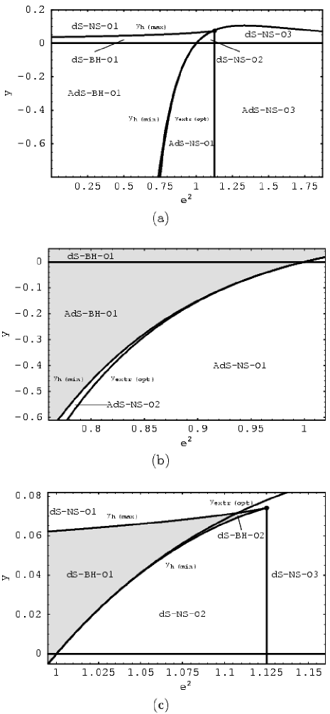
Figure 16: The classification of the Reissner–Nordström–(anti-)de Sitter spacetimes according to the properties of the embedding diagrams of the associated optical reference geometry. The functions $y_{\mathrm{h(min)}}(e)$ and $y_{\mathrm{h(max)}}(e)$ limit the region of black-hole spacetimes (shaded) in the parameter space $e^{2}$-$y$, and they separate spacetimes of different type of the embeddings, along with the function $y_{\mathrm{extr(opt)}}(e)$, and the lines $y=0$ (for $e^{2}\geq 0$) and $e^{2}=9/8$ (for $y<2/27$).

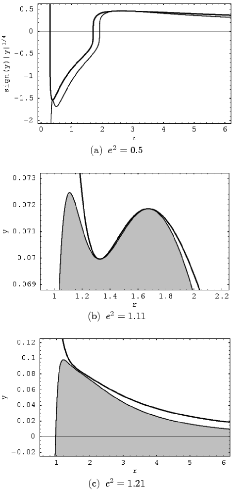
Figure 17: Embeddability of the optical reference geometry associated with the Reissner–Nordström–(anti-)de Sitter spacetimes. According to the value of the charge parameter $e^{2}$, there are three qualitatively different types of the behaviour of the functions $y_{\mathrm{h}}(r;e)$ (bold lines) and $y_{\mathrm{e(opt)}}(r;e)$ (thin solid lines) determining the regions of embeddability. The regions of embeddability are shaded. Turning points of the embedding diagrams correspond to the photon circular orbits located at radii given by the local extrema of $y_{\mathrm{h}}(r;e)$.

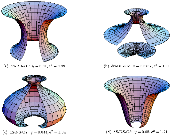
Figure 18: Typical embedding diagrams of the optical reference geometry of the asymptotically de Sitter spacetimes. In the black-hole spacetimes a limited region between the outer black-hole horizon and the cosmological horizon can be embedded, and some part of the region between the singularity and the inner black-hole horizon can be embedded in the type of dS-BH-O2 (case (b)). For naked-singularity spacetimes, a limited region between the singularity and the cosmological horizon can be embedded. However, for the type of dS-NS-O1, no region of the optical geometry can be embedded into the Euclidean space. Turning points of the embedding diagrams correspond to the radii of the photon circular geodesics, which are independent of the cosmological parameter $y$. The centrifugal force vanishes there; within the upward (inward) sloping areas of the embedding diagram the centrifugal force is outward (inward) directed.

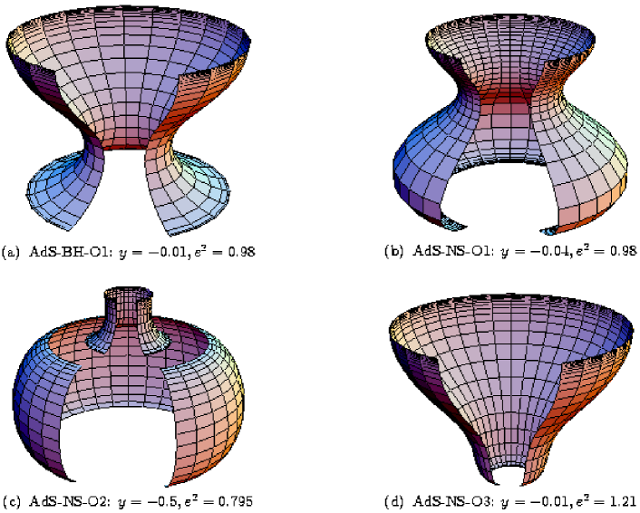
Figure 19: Typical embedding diagrams of the optical reference geometry of the asymptotically anti-de Sitter spacetimes. There is one type of the embedding for black holes (case (a)), and three types of the embedding for naked singularities (cases (b) through (d)). In all of these cases, the embedding is possible for $r\to\infty$, however, it is shrunk to a finite value of the embedding coordinate $\rho$, depending on the cosmological parameter $y$. Turning points of the embedding diagrams correspond to the radii of the photon circular geodesics, which are independent of $y$. Behavior of the centrifugal force is governed by the same rules as in the case of asymptotically de Sitter spacetimes.

In the parameter space $e^{2}$-$y$, distribution of types of the Reissner–Nordström–(anti-)de Sitter spacetimes with different properties of the embedding diagrams of their optical geometry is given in Fig. 16. Typical embedding diagrams are constructed by a numerical code and presented in Figs 18 and 19. Properties of the embedding diagrams of the optical geometry can be summarized in the following way.

A1 Reissner–Nordström–de Sitter black-hole spacetimes

There are two types of the black-hole spacetimes (dS-BH-O1 and 2). For both of them, the embedding diagram has a throat between the outer black-hole horizon and the cosmological horizon. None of the embedding diagrams can reach any of the event horizons. For the spacetimes of the type dS-BH-O1 (with $e^{2}\leq 1$), the embedding is not possible under the inner horizon, while in the spacetimes dS-BH-O2 ($1<e^{2}\leq 9/8$), some part of the region between the singularity at $r=0$ and the inner horizon can be embedded. The character of the embedding in the case of dS-BH-O1 spacetimes is just the same as in the case of Schwarzschild–de Sitter black holes. For dS-BH-O2 spacetimes the difference is given by the inner part of the embedding. In the case of Reissner-Nordström black-hole spacetimes, the embedding can be extended up to $r\to\infty$. Typical embedding diagrams are constructed by a numerical procedure and given in Fig. 18a (dS-BH-O1) and Fig. 18b (dS-BH-O2).

A2 Reissner–Nordström–de Sitter naked-singularity spacetimes

There are three types of naked-singularity spacetimes. In the type dS-NS-O1 spacetimes no embedding is admitted. In the type dS-NS-O2 spacetimes, the embedding has a belly and a throat (Fig. 18c). In the type dS-NS-O3 spacetimes, there are no turning points of the embedding diagrams (Fig. 18d). The embedding does not reach neither the singularity and the cosmological horizon in both dS-NS-2 and 3 spacetimes. This is the only difference with the embeddings of Reissner–Nordström naked-singularity spacetimes, where the embedding can be extended up to $r\to\infty$.

B1 Reissner–Nordström–anti-de Sitter black-hole spacetimes

There is only one type of the black-hole spacetimes denoted AdS-BH-O1. A typical embedding is shown in Fig. 19a. The embedding extends from some radius above the outer horizon up to infinity and has a throat. The embedding is not allowed in the region under the inner horizon. Notice that the embedding diagrams of both black-hole and naked-singularity backgrounds in the asymptotically anti-de Sitter universe has a specific property given by the definition of the embedding coordinate $\rho$ (see Eq. (98)). The embedding diagrams cover whole the asymptotic part of spacetime in a restricted part of the Euclidean space. There is

$$\rho(r\to\infty)=(-y)^{-1/2}.$$ (111)

Clearly, with decreasing attractive cosmological constant the embedding diagram is deformed with increasing intensity. The circles of $r=\mathrm{const}$ are concentrated with an increasing density around $\rho=(-y)^{-1/2}$ as $r\to\infty$. This behavior is exactly the same as in the case of Schwarzschild–anti-de Sitter black holes, and it represents the only difference with respect to the case of Reissner–Nordström black holes.

B2 Reissner–Nordström–anti-de Sitter naked-singularity spacetimes

There are three types of naked-singularity spacetimes. In the type AdS-NS-O1 spacetimes, the embedding is continuously extended between the inner boundary given by the function $y_{\mathrm{e(opt)}}(r;e)$ and infinity, and has a belly and a throat (Fig. 19b). In the type of AdS-NS-O2 spacetimes, the embedding is separated into two parts—the inner one has a belly, the outer one has a throat (Fig. 19c). In the type of AdS-NS-O3 spacetimes, the embedding is continuously extended between the inner boundary given by $y_{\mathrm{e(opt)}}(r;e)$ and infinity, but it has no turning point (Fig. 19d). The difference with respect to embeddings of the Reissner–Nordström naked-singularity spacetimes is given by AdS-NS-O2 spacetimes, where the embedding has two parts, and by the asymptotic behavior of the embedding diagram in all the type AdS-NS-O1 through 3 spacetimes.

8 Asymptotic behavior of the optical geometry

The reason why the embedding into the Euclidean space is not possible in some parts of the optical (or ordinary) geometry is explained in [12, 14]. However, the optical geometry is still well defined outside the regions of the embeddability into Euclidean space nearby the event horizons. It is possible to demonstrate its properties by the behavior of the proper lengths along the radial direction. In the optical geometry, the proper radial length coincides with the well known Regge–Wheeler ‘tortoise’ coordinate

$$r^{\ast}=\int\left(1-\frac{2}{r}+\frac{e^{2}}{r^{2}}-yr^{2}\right)^{-1}\mathrm{d}r.$$ (112)

This gives direct relevance of the ‘tortoise’ coordinate in the optical space, since it can be shown that in the black-hole spacetimes, the outer black-hole horizon and the cosmological horizon are infinitely far away in the optical geometry. At $r\sim r_{\mathrm{b}+}$, there is $r^{\ast}\sim+\ln|r-r_{\mathrm{b}+}|\to-\infty$, while at $r\sim r_{\mathrm{c}}$, there is $r^{\ast}\sim-\ln|r_{\mathrm{c}}-r|\to+\infty$. On the other hand, in the ordinary geometry, the horizons are located at a finite proper radial distance

$$\tilde{r}=\int\left(1-\frac{2}{r}+\frac{e^{2}}{r^{2}}-yr^{2}\right)^{-1/2}\mathrm{d}r;$$ (113)

at $r\sim r_{\mathrm{b}+}$, $\tilde{r}\sim\sqrt{r-r_{\mathrm{b}+}}$, and at $r\sim r_{\mathrm{c}}$, $\tilde{r}\sim\sqrt{|r_{\mathrm{c}}-r|}$. In the Reissner–Nordström–de Sitter spacetimes, the optical geometry extends infinitely beyond the limit of embeddability, approaching asymptotically the geometry

$$\mathrm{d}\tilde{\sigma}^{2}\approx\mathrm{d}r^{\ast^{2}}+C_{1}\exp\left[-r^{\ast}/C(r_{\mathrm{b}+})\right]\left(\mathrm{d}\theta^{2}+\sin^{2}\theta\,\mathrm{d}\phi^{2}\right)$$ (114)

for $r\to r_{\mathrm{b}+}$, $r^{\ast}\to-\infty$, and

$$\mathrm{d}\tilde{\sigma}^{2}\approx\mathrm{d}r^{\ast^{2}}+C_{2}\exp\left[-r^{\ast}/C(r_{\mathrm{c}})\right]\left(\mathrm{d}\theta^{2}+\sin^{2}\theta\,\mathrm{d}\phi^{2}\right)$$ (115)

for $r\to r_{\mathrm{c}}$, $r^{\ast}\to+\infty$; $C_{1}$, $C_{2}$ and $C(r_{\mathrm{b}+})$, $C(r_{\mathrm{c}})$ are constants given in terms of the parameters of the spacetime.

For Reissner–Nordström–anti-de Sitter black holes, the optical space has again the property that at $r\sim r_{\mathrm{b}+}$, there is $r^{\ast}\sim\ln|r-r_{\mathrm{b}+}|\to-\infty$, while for $r\to\infty$, there is $r^{\ast}\sim(-y)^{-1}\ln r\to+\infty$, and the asymptotical behavior of the optical geometry is determined by formulae similar to Eqs (114) and (115), respectively.

In the vicinity of the inner black-hole horizon, $r\to r_{\mathrm{b}-}$, there is $r^{\ast}\sim-\ln|r_{\mathrm{b}-}-r|$ and the optical geometry has the asymptotical form similar to (114). On the other hand, for $r\to 0$, there is $r^{\ast}\sim r^{3}/3e^{2}\to 0$ independently of the value of $y\neq 0$. At $r\to 0$, the asymptotic form of the optical geometry of the spacetimes with $e^{2}\neq 0$ is given by

$$\mathrm{d}\tilde{\sigma}^{2}\approx\mathrm{d}r^{\ast^{2}}+\frac{r^{4}}{e^{2}}\left(\mathrm{d}\theta^{2}+\sin^{2}\theta\,\mathrm{d}\phi^{2}\right).$$ (116)

In the naked singularity spacetimes, the asymptotic form of $r^{\ast}$ and $\mathrm{d}\tilde{\sigma}^{2}$ at $r\to r_{\mathrm{c}}$ (for $y>0$), and at $r\to\infty$ (for $y<0$), respectively, is the same as in the black-hole spacetimes, i.e., $r^{\ast}\to+\infty$ and there is no other divergence of the ‘tortoise’ coordinate in the naked-singularity spacetimes. There is $r^{\ast}\sim r^{3}/3e^{2}\to 0$ for $r\to 0$. At $r\sim 0$, the optical geometry is again determined by the formula (116).

9 Concluding remarks

The Reissner–Nordström–(anti-)de Sitter spacetimes can be separated into eleven types of spacetimes with qualitatively different character of the geodetical motion. Properties of the motion can be summarized and compared with the properties of the motion in the Schwarzschild–de Sitter and the Reissner–Nordström spacetimes in the following way.

(1) The motion above the outer horizon of black-hole backgrounds has the same character as in the Schwarzschild–(anti-)de Sitter spacetimes for both asymptotically de Sitter ($y>0$) and anti-de Sitter ($y<0$) spacetimes. Namely, there is only one static radius (giving limits on existence of circular geodetical motion) for $y>0$, and no static radius for $y<0$. No static radius is possible under the inner black-hole horizon for both $y>0$ and $y<0$, no circular geodesics are possible there. Only one photon circular orbit exists above the outer horizon for both $y>0$, and $y<0$; its radius is, moreover, independent of $y$. No photon circular orbit can exist under the inner black-hole horizon for both $y>0$, and $y<0$. From the astrophysical point of view, the most important are stable circular orbits as they allow accretion processes in the disk regime. In all of the asymptotically anti-de Sitter black-hole spacetimes, the stable circular orbits exist in a region above the outer horizon and can be extended up to $r\to\infty$ in the limit of ultrarelativistic particles. In the case of asymptotically de Sitter black-hole spacetimes, there is a region of stable circular orbits limited both from below and from above by the function $y_{\mathrm{ms}}(r;e)$. The stable circular orbits can exist only for small values of the cosmological parameter $y<y_{\mathrm{ms(bh)}}=0.000693$, with allowed values of the charge parameter $e^{2}<e^{2}_{\mathrm{ms(bh)}}=1.000695$. The presence of an outer marginally stable circular geodesic allows outflow of matter from accretion disks and is, therefore, of high astrophysical importance [30].

(2) The motion in the naked-singularity backgrounds has similar character as the motion in the field of Reissner–Nordström naked singularities. However, in the case of $y>0$, two static radii can exist, while the Reissner–Nordström naked singularities contain one static radius only. The outer static radius appears due to the effect of the repulsive cosmological constant. On the other hand, the inner static radius, located nearby the ring singularity, survives even in the presence of an attractive cosmological constant. Two photon circular orbits exist in naked singularity backgrounds for both $y>0$, and $y<0$, if $1<e^{2}<9/8$, just as in the field of Reissner–Nordström naked singularities. Stable circular orbits exist in all of the naked-singularity spacetimes. In the spacetimes with $e^{2}>5/4$ and $y<0$, there are stable circular geodesics only. On the other hand, if $e^{2}<5/4$ and $y_{\mathrm{ms(min)}}<y<y_{\mathrm{ms(max)}}$, there are even two separated regions of stable circular geodesics, with the inner one being limited by the inner static radius from bellow, where particles with zero angular momentum (in stable equilibrium positions) are located. In the asymptotically de Sitter naked-singularity spacetimes, two regions of stable circular orbits can exist, if $e^{2}<275/216$, and $y<0.00174$; otherwise, the inner region of stable circular orbits survives. More details can be extracted directly from Fig. 3.

(3) In the black-hole spacetimes, escape photon cones has the same character as in the Schwarzschild–(anti-)de Sitter spacetimes. In the asymptotically anti-de Sitter spacetimes, the capture cone remains nonzero as $r\to\infty$ due to the effect of the attractive cosmological constant. In the naked-singularity spacetimes, the escape photon cones are determined by the presence of the unstable photon circular orbits—in the region located under the radius of the unstable photon circular orbit, directional angles corresponding to bound photons appear. The cone of bound photons is most extended at the radius corresponding to the stable circular photon orbit (note that photon circular orbits exist, if $e^{2}<9/8$). In spacetimes with $e^{2}>9/8$, all photons escape, except those radially incoming into the singularity at $r=0$.

The embedding diagrams of both ordinary and optical reference geometry give clear illustration of the influence of both the charge and cosmological parameter on the structure of the Reissner–Nordström–(anti-)de Sitter spacetimes.

(1) For the ordinary geometry, the embedding is impossible for Reissner–Nordström–anti-de Sitter naked singularities with $y<y_{\mathrm{e(ord)(min)}}(e)$. For all values of $y<0$, and $y>0$, the embedding is impossible in vicinity of $r=0$. In the asymptotically anti-de Sitter black-hole and naked-singularity spacetimes, the embeddability is limited from above, too. In the asymptotically de Sitter black-hole and naked-singularity spacetimes, the embeddability is possible up to the cosmological horizon. The embedding diagram resembles a funnel with a throat near the cosmological horizon—with $y$ increasing, the funnel becomes shrunk and flattened.

(2) For the optical reference geometry, the embedding is possible for all of the Reissner–Nordström–anti-de Sitter black holes and naked singularities from the below limit nearby $r=0$ up to infinity, although, it is deformed by shrinking of the asymptotic region to vicinity of finite value of the embedding radial coordinate $\rho=(-y)^{-1/2}$. On the other hand, the embeddability is not possible for the Reissner–Nordström–de Sitter naked singularity spacetimes with $e^{2}>9/8$ and $y>(e^{2}-1)/e^{8}$. Further, for the naked singularity spacetimes with $e^{2}<9/8$, and both $y>0$ and $y<0$, the embedding diagrams have a throat and a belly. In some cases the embedding for naked singularities with $y<0$ is discontinuous, it consists from two parts. For black holes (with both $y>0$ and $y<0$), the embedding diagram has a throat, the embedding cannot reach both the inner and outer black-hole horizon. If $y>0$, the embedding cannot reach the cosmological horizon, too. If $y<0$, no part of the space under the inner horizon can be embedded.

Embedding diagrams of the optical geometry give an important tool of visualization and clarification of the dynamical behavior of test particles moving along equatorial circular orbits: we imagine that the motion is constrained to the surface $z(\rho)$ [12]. The shape of the embedding surface $z(\rho)$ is directly related to the centrifugal acceleration. Within the upward sloping areas of the embedding diagram, the centrifugal acceleration points towards increasing values of $r$, and the dynamics of test particles has an essentially Newtonian character. However, within the downward sloping areas of the embedding diagrams, the centrifugal acceleration has a radically non-Newtonian character as it points towards decreasing values of $r$. Such a kind of behavior appears where the diagrams have a throat and a belly. At the turning points of the embedding diagrams, where $\mathrm{d}z/\mathrm{d}\rho=0$, the centrifugal acceleration vanishes and changes its sign.

We can understand this connection between the centrifugal force and the embedding of the optical space in terms of the radius of gyration representing rotational properties of rigid bodies [26]. In Newtonian physics, the gyration radius $\tilde{r}$ is defined by the relation

$$\tilde{r}=\sqrt{\frac{\ell}{\Omega}}.$$ (117)

where $\ell=J/M$ is the specific angular momentum of a rigid body ($J$ is angular momentum of the body, $M$ is its mass) rotating with angular velocity $\Omega$, i.e., it is defined as the radius $\tilde{r}$ of the circular orbit on which a point-like particle having the same mass $M$ and angular velocity $\Omega$ would have the same angular momentum $J=M{\tilde{r}}^{2}\Omega$.

In Newtonian physics, radius of gyration equals both the circumferential radius and the radius given by proper radial distance from the rotational axis, however, in General Relativity they differ. The radius of gyration is convenient for understanding the dynamical effects of rotation in the framework of General Relativity, as the direction of increasing $\tilde{r}$ defines the local outward direction of these effects. The surfaces $\tilde{r}=\mathrm{const}$, called von Zeipel cylinders, proved to be a very useful concept in the theory of rotating fluids in stationary, axially symmetric spacetimes. In Newtonian physics, these are ordinary straight cylinders but their shape is deformed by general-relativistic effects and their topology may be noncylindrical. There is a critical family of self-crossing von Zeipel surfaces [31].

The close relation of the centrifugal force, and the embedding diagrams of the equatorial plane of the optical geometry follows directly from the fact that the embedding diagrams are expressed in terms of the radius of gyration

$$[\tilde{h}_{\phi\phi}(\theta=\pi/2)]^{1/2}=\rho=\tilde{r},$$ (118)

and the radial component of the centrifugal force in the equatorial plane is also related to the radius of gyration

$$Z_{\mathrm{R}}(r)\sim\tilde{r}^{-1}\partial_{r}\tilde{r}.$$ (119)

The turning points of the embedding diagrams determine both radii where the centrifugal force changes its sign and the radii of cusps where the critical von Zeipel surfaces are self-crossing. Therefore, the embedding diagrams also reflect the properties of perfect fluid orbiting black holes or naked singularities.

We can conclude that in most cases the phenomena connected with geodetical motion and embedding diagrams in the Reissner–Nordström and Schwarzschild–(anti-)de Sitter spacetimes are incorporated into the corresponding phenomena in the Reissner–Nordström–(anti-)de Sitter spacetimes in an additive way. However, in some cases, new phenomena appear as a qualitatively new result of the interplay of the effect of appropriately tuned values of the electric charge and the cosmological constant.

For the geodetical motion, the additive way is realized in most of the cases considered here. The qualitatively new features caused by an interplay of the charge and the cosmological constant are the following: the existence of asymptotically de Sitter black holes with unstable circular geodesics only, the existence of asymptotically de Sitter naked singularities with an internal region of stable circular geodesics and an external region of unstable circular geodesics (if $e^{2}<9/8$, these regions are separated, if $e^{2}>9/8$, they are continuously matched).

For the embedding diagrams, among these qualitatively new phenomena the following can be ascribed: the nonexistence of embedding diagrams of the ordinary space for some naked singularities with $y<0$, and nonexistence of embedding diagrams of the optical space for some naked singularities with $y>0$. Existence of separated parts of the embedding diagrams of the optical space of some naked singularities with $y<0$.

In the presented work, attention has been focused on embedding of the ordinary and optical geometry and the geodetical motion in the Reissner–Nordström–(anti-)de Sitter spacetimes, reflecting the combined effect of an electric charge and a nonzero cosmological constant an the character of black-hole and naked-singularity spacetimes. A simple case of equilibrium positions of charged (and spinning) test particles in these spacetimes has been discussed in [32], where it has been shown that the equilibria are independent of the spin of the test particles. The motion of charged test particles is a more complex problem, and it is under study at present.

The combined effect of rotation and a nonzero cosmological constant in the black-hole and naked-singularity spacetimes has been extensively studied for the equatorial photon motion [33, 34]. The general geodetical motion and embeddings of the ordinary and optical geometry are under study at present.

This work was partly supported by the GAČR grant No. 202/02/0735/A, the Committee for collaboration of Czech Republic with CERN and the Bergen Computational Physics Laboratory in the framework of the European Community—Access to Research Infrastructure action of the Improving Human Potential Programme. The authors would like to express their gratitude to the Theory Division of CERN, where an essential part of the work has been done, and to the BCPL at the University of Bergen, where the work has been finished, for perfect hospitality.

References

- [1] L. M. Krauss, M. S. Turner: Gen. Relativity Gravitation 27 (1995) 1137
- [2] J. P. Ostriker, P. J. Steinhardt: Nature 377 (1995) 600
- [3] N. Bahcall, J. P. Ostriker, S. Perlmutter, P. J. Steinhardt: Science 284 (1999) 1481
- [4] R. R. Caldwell, R. Dave, P. J. Steinhardt: Phys. Rev. Lett. 80 (1998) 1582
- [5] L. Wang, R. R. Caldwell, J. P. Ostriker, P. J. Steinhardt: Astrophys. J. 530 (2000) 17
- [6] C. Armendariz-Picon, V. Mukhanov, P. J. Steinhardt: Phys. Rev. Lett. 85 (2000) 4438
- [7] A. Sen: In: 29th International Conference on High Energy Physics, Vancouver, 23–29 July 1998, eds. A. Astbury, D. Axen, J. Robinson, Singapore (1999). World Scientific
- [8] C. Schmidhuber: Nuclear Phys. B 580 (2000) 140
- [9] C. W. Misner, K. S. Thorne, J. A. Wheeler: Gravitation: Freeman, San Francisco (1973)
- [10] M. A. Abramowicz, B. Carter, J.-P. Lasota: Gen. Relativity Gravitation 20 (1988) 1173
- [11] M. A. Abramowicz: Monthly Notices Roy. Astronom. Soc. 256 (1992) 710
- [12] S. Kristiansson, S. Sonego, M. A. Abramowicz: Gen. Relativity Gravitation 30 (1998) 275
- [13] Z. Stuchlík, S. Hledík: Classical Quantum Gravity 16 (1999) 1377
- [14] Z. Stuchlík, S. Hledík: Phys. Rev. D 60 (1999) 044006 (15 pages)
- [15] Z. Stuchlík, S. Hledík, J. Juráň: Classical Quantum Gravity 17 (2000) 2691
- [16] Z. Stuchlík, S. Hledík, J. Šoltés, E. Østgaard: Phys. Rev. D 64 (2001) 044004 (17 pages)
- [17] R. Penrose: Nuovo Cimento B 1 (1969) 252
- [18] F. de Felice: Astronomy and Astrophysics 34 (1974) 15
- [19] M. A. Abramowicz, P. Nurowski, N. Wex: Classical Quantum Gravity 10 (1993) L183
- [20] M. A. Abramowicz, A. R. Prasanna: Monthly Notices Roy. Astronom. Soc. 245 (1990) 720
- [21] M. A. Abramowicz, P. Nurowski, N. Wex: Classical Quantum Gravity 12 (1995) 1467
- [22] J. M. Aguirregabiria, A. Chamorro, K. R. Nayak, J. Suinaga, C. V. Vishveshwara: Classical Quantum Gravity 13 (1996) 2179
- [23] Z. Stuchlík: Bull. Astronom. Inst. Czechoslovakia 41 (1990) 341
- [24] M. A. Abramowicz, J. Bičák: Gen. Relativity Gravitation 23 (1991) 941
- [25] S. Sonego, M. A. Abramowicz: J. Math. Phys. 39 (1998) 3158
- [26] M. A. Abramowicz, J. Miller, Z. Stuchlík: Phys. Rev. D 47 (1993) 1440
- [27] O. Semerák: Nuovo Cimento B 110 (1995) 973
- [28] R. T. Jantzen, P. Carini, D. Bini: Ann. Physics 215 (1992) 1
- [29] M. A. Abramowicz: Monthly Notices Roy. Astronom. Soc. 245 (1990) 733
- [30] Z. Stuchlík, P. Slaný, S. Hledík: Astronomy and Astrophysics 363 (2000) 425
- [31] M. Kozłowski, M. Jaroszyński, M. A. Abramowicz: Astronomy and Astrophysics 63 (1978) 209
- [32] Z. Stuchlík, S. Hledík: Phys. Rev. D 64 (2001) 104016 (12 pages)
- [33] Z. Stuchlík, G. Bao, E. Østgaard, S. Hledík: Phys. Rev. D 58 (1998) 084003
- [34] Z. Stuchlík, S. Hledík: Classical Quantum Gravity 17 (2000) 4541