Global m=1 instabilities and lopsidedness in disc galaxies

Abstract

Lopsidedness is common in spiral galaxies. Often, there is no obvious external cause, such as an interaction with a nearby galaxy, for such features. Alternatively, the lopsidedness may have an internal cause, such as a dynamical instability. In order to explore this idea, we have developed a computer code that searches for self-consistent perturbations in razor-thin disc galaxies and performed a thorough mode-analysis of a suite of dynamical models for disc galaxies embedded in an inert dark-matter halo with varying amounts of rotation and radial anisotropy.

Models with two equal-mass counter-rotating discs and fully rotating models both show growing lopsided modes. For the counter-rotating models, this is the well-known counter-rotating instability, becoming weaker as the net rotation increases. The $m=1$ mode of the maximally rotating models, on the other hand, becomes stronger with increasing net rotation. This rotating $m=1$ mode is reminiscent of the eccentricity instability in near-Keplerian discs.

To unravel the physical origin of these two different $m=1$ instabilities, we studied the individual stellar orbits in the perturbed potential and found that the presence of the perturbation gives rise to a very rich orbital behaviour. In the linear regime, both instabilities are supported by aligned loop orbits. In the non-linear regime, other orbit families exist that can help support the modes. In terms of density waves, the counter-rotating $m=1$ mode is due to a purely growing Jeans-type instability. The rotating $m=1$ mode, on the other hand, grows as a result of the swing amplifier working inside the resonance cavity that extends from the disc center out to the radius where non-rotating waves are stabilized by the model’s outwardly rising $Q$-profile.

1 Introduction

The stellar and/or gaseous discs of spiral galaxies are often affected by large-scale asymmetries. About half of all late-type galaxies show a lopsided structure that affects the whole disc (Richter & Sancisi, 1994; Haynes et al., 1998). Based on near-infrared images of a sample of 149 disc galaxies, Bournaud et al. (2005) find that a large fraction of them have asymmetric stellar discs. The strength of the lopsidedness does not correlate with the presence of companions but, instead, correlates with the presence of bars and spiral arms. They explore three different causes for the lopsidedness: galaxy interactions, galaxy mergers, and gas accretion. These authors favour the latter explanation, which indeed can trigger strong lopsidedness if the gas in-fall is sufficiently asymmetric. Angiras et al. (2006) analysed Hi surface density maps and R-band images of 18 galaxies in the Eridanus group. All galaxies showed significant lopsidedness in their Hi discs. Where the stellar and gaseous discs overlap, their asymmetries are comparably strong. Since the Eridanus group galaxies are more strongly lopsided than field galaxies, these authors conclude that tidal interaction in the group environment may contribute to generating lopsidedness in disc galaxies. Swaters et al. (1999) studied kinematic lopsidedness in two spiral galaxies and argued that it may be related to lopsidedness in the potential. Alternatively, the stellar disc may lie off-centre in the halo’s gravitational potential well and spin in a sense retrograde to its orbit about the halo centre (Levine & Sparke, 1998). Lopsided structures are not the prerogative of disc galaxies alone. In some nucleated dwarf elliptical galaxies, for instance, the nucleus is displaced with respect to the centre of the outer isophotes (Binggeli et al., 2000). While some authors regard these displaced nuclei as being globular clusters projected close to the galaxy photocenter (Côté et al., 2006), in some cases, such as the Fornax dwarf elliptical FCC046, there are clear indications that the nucleus is an integral part of the galaxy’s stellar body and is displaced by a mechanism that affects the whole galaxy (De Rijcke & Debattista, 2004).

Sellwood & Valluri (1997) used N-body simulations to investigate the stability of a family of oblate elliptical galaxy models and found that a strong lopsided instability occurs in models with small radial anisotropy and strong counter-rotation. This instability may cause lopsidedness in stellar systems with no or small net rotation, such as dwarf ellipticals (De Rijcke & Debattista, 2004). Bertola & Corsini (1999) compiled a list of several types of counter-rotation in galaxies of different morphological type. They regard counter-rotation of stellar vs. stellar discs as the prevailing type of counter-rotation since it is the end state of a galaxy with an embedded counter-rotating star-forming gas disc.

Rubin et al. (1992) discovered in the S0 galaxy NGC4550 two distinct stellar components rotating in opposite directions. Another example is the normal Sab galaxy NGC7217 (Merrifield and Kuijken, 1994). Vergani et al. (2007) present the case of NGC5713, a Sbc spiral galaxy in which 20 % of the stars are on retrograde orbits. Their data suggest that NGC5713 accreted neutral gas from its surroundings on retrograde orbits. This gas was subsequently converted into stars in a counter-rotating disc. Less than 10 % of all S0s host counter-rotating stellar populations while counter-rotating gas is found in roughly one quarter of them (Kuijken et al., 1996). Kannappan & Fabricant (2001) find 4 counter-rotators among a sample of 17 elliptical and lenticular galaxies. They find no counter-rotation among 38 Sa-Sbc galaxies.

An axisymmetric galactic disc perturbed by a constant lopsided halo potential causes a net lopsided distribution in the disc, opposite to the perturbation halo potential (Jog, 1997, 1999). Tremaine & Yu (2000) suggest that counter-rotation can be produced when a triaxial halo with an initially retrograde pattern speed slowly changes to a pro-grade pattern speed. This is a situation that probably does not occur very often. Moreover, this mechanism requires evolution on long timescales of the order of $\sim 10^{10}$ yr. Overall, counter-rotation is detected only rarely in disc galaxies. Hence, the lopsidedness observed in so many disc galaxy is most likely not caused by counter-rotation.

In this paper, we investigate the role played by instabilities in generating lopsidedness in isolated disc galaxies using a semi-analytic matrix method developed by Vauterin & Dejonghe (1996). More specifically, we want to explore whether lopsided instabilities can be triggered in fully rotating disc galaxies. In the next section, we introduce the formalism underlying the computer code that we developed to analyse the stability of a given dynamical model for a disc galaxy. In section 3, we present the unperturbed toy galaxy models whose stability is analysed in section 4. We investigate under what physical circumstances (i.e. degree of counter-rotation and orbital anisotropy) lopsided structures can spontaneously grow in these disc galaxy models. In section 5, we give a physical explanation for the self-consistent growth of lopsided structures, based on the response of individual stellar orbits to the growing instability. We summarise our conclusions in section 6.

2 Searching for instabilities

We have developed a computer code to analyse the stability of razor-thin stellar discs embedded in an axisymmetric or spherical dark matter halo. The halo is assumed to be dynamically too hot to develop any instabilities. This inert halo only enters the calculations by its contribution to the global gravitational potential. We only consider the stellar component of the disc and neglect the dynamical influence of gas and dust.

We describe an instability as the superposition of a time-independent axisymmetric equilibrium configuration and a perturbation that is sufficiently small to warrant the linearisation of the Boltzmann equation. The equilibrium configuration is characterised completely by the global potential $V_{0}(r)$ and the distribution function $f_{0}(E,J)$, with binding energy $E$ and angular momentum $J$. A general perturbing potential can be expanded in a series of normal modes of the form

$$V^{\prime}(r,\theta,t)=V^{\prime}(r)e^{i(m\theta-\omega t)},$$ (1)

with a pattern speed $\Re(\omega)/m$ and a growth rate $\Im(\omega)$, that, owing to the linearity of the relevant equations, can be studied independently from each other. We write the response of the distribution function to a perturbation as:

$$f(r,\theta,v_{r},v_{\theta},t)=f_{0}(E,J)+f^{\prime}(r,\theta,v_{r},v_{\theta},t).$$ (2)

The evolution of the perturbed part of the distribution function is calculated using the linearised collision-less Boltzmann equation:

$$\frac{\partial f^{\prime}}{\partial t}-[f^{\prime},E]=[f_{0},V^{\prime}].$$ (3)

We rewrite the right-hand side of the last equation as:

$$[f_{0},V,] = -\nabla_{\mathbf{v}}f_{0}\cdot\nabla_{\mathbf{r}}V^{\prime}$$ (4)

$$= -(\frac{\partial f_{0}}{\partial E}\nabla_{\mathbf{v}}E+\frac{\partial f_{0}}{\partial J}\nabla_{\mathbf{v}}J)\cdot\nabla_{\mathbf{r}}V^{\prime}$$

$$= \frac{\partial f_{0}}{\partial E}\mathbf{v}\cdot\nabla_{\mathbf{r}}V^{\prime}-\frac{\partial f_{0}}{\partial J}\frac{\partial V^{\prime}}{\partial\theta}.$$

We also know that:

$$\nabla_{\mathbf{r}}V^{\prime}\cdot\mathbf{v}=\frac{\rm{d}V^{\prime}}{\rm{d}t}-\frac{\partial V^{\prime}}{\partial t}.$$ (5)

With this last identity, equation (3) becomes:

$$\frac{\partial f^{\prime}}{\partial t}-[f^{\prime},E]=\frac{\partial f_{0}}{\partial E}\frac{\rm{d}V^{\prime}}{\rm{d}t}+i(\omega\frac{\partial f_{0}}{\partial E}-m\frac{\partial f_{0}}{\partial J})V^{\prime}.$$ (6)

The left-hand side of eq. (6) is simply the total time derivative of $f^{\prime}$ along an unperturbed orbit. If we integrate eq. (6) along the unperturbed orbits, we immediately obtain the response of the distribution function to the perturbing potential given by eq. (1):

$$f^{\prime}(\mathbf{r}_{0},\mathbf{v}_{0};t_{0})=$$

$$\frac{\partial f_{0}}{\partial E}V^{\prime}(\mathbf{r}_{0};t_{0})+i(\omega\frac{\partial f_{0}}{\partial E}-m\frac{\partial f_{0}}{\partial J})\int_{-\infty}^{t_{0}}V^{\prime}(r)e^{i(m\theta-\omega t)}{\rm{d}}\,t.$$ (7)

The integral in eq. (7) converges if the perturbation disappears for $t\rightarrow-\infty$ and is growing sufficiently fast in time ($\Im(\omega)>0$).

Along an unperturbed orbit, the radial coordinate $r$ is a periodic function of time with angular frequency $\omega_{r}$, just like $v_{r}$ and $v_{\theta}$. Because the mean value of $v_{\theta}$ can be different from zero, $\theta$ will be the superposition of a periodic function $\theta_{p}(t)$ and a uniform drift velocity $\omega_{\theta}$:

$$\theta=\omega_{\theta}t+\theta_{p}(t).$$ (8)

We separate the part of the integrand in eq. (7) that is periodic with frequency $\omega_{r}$ from the aperiodic part and expand it in a Fourier series:

$$V^{\prime}(r)e^{i(m\theta-\omega t)} = I(t)e^{i(m\omega_{\theta}-\omega)t}$$ (9)

$$= e^{i(m\omega_{\theta}-\omega)t}\sum_{l=-\infty}^{\infty}I_{l}e^{il\omega_{r}t}.$$

The coefficients $I_{l}$ are given by

$$I_{l}=\frac{1}{T}\int_{0}^{T}I(t)e^{-il\omega_{r}t}\,{\rm d}t,$$ (10)

where the integration extends over half a radial period, starting at apocentre at $t=0$.

The first term of the right-hand side of equation (7) is rewritten as:

$$\frac{\partial f_{0}}{\partial E}V^{\prime}(\mathbf{r}_{0};t_{0}) = \frac{\partial f_{0}}{\partial E}e^{i(m\theta_{0}-\omega t_{0})}\int_{-\infty}^{0}{\rm{d}}[I(t)e^{i(m\omega_{\theta}-\omega)t}]$$ (11)

$$= \frac{\partial f_{0}}{\partial E}e^{i(m\theta_{0}-\omega t_{0})}\sum_{l=-\infty}^{\infty}I_{l}.$$

The orbits are integrated in the unperturbed potential using a leapfrog method. Instead of using $E$ and $J$, orbits in the unperturbed potential are catalogued by their apocentre and pericentre distances, denoted by $r_{+}$ and $r_{-}$, respectively. The sense of rotation is indicated by the sign of $r_{-}$. The grid of the orbit catalogue is given by $(r_{+},r_{-})\in[0,r_{\rm max}]\times[-r_{+},r_{+}]$. We use a grid of $100\times 200$ cells. For every orbit, $\omega_{r}$ and $\omega_{\theta}$ are determined, the Fourier expansion (9) is performed up to the order of $l_{\rm max}=50$, and the coefficients are stored. If we want to calculate the response of the distribution function in the point $(\mathbf{r}_{0},\mathbf{v}_{0})$ in phase space at time $t_{0}$, we choose an orbit from the catalogue with the correct integrals of motion (i.e. $r_{+}$ and $r_{-}$) but passing through its apocentre at $t=0$ so the actual orbit has an offset in time $t(r_{0})$ and azimuth $\theta_{p}(r_{0})$ that must be taken into account. Therefore we also store a tabulation of $t(r)$ and $\theta_{p}(r)$.

The response of the distribution function to the perturbation now assumes the following concise form:

$$f^{\prime}(\mathbf{r}_{0},\mathbf{v}_{0};t_{0}) = e^{i(m\theta_{0}-\omega t_{0})}\times$$ (12)

$$\sum_{l=-\infty}^{\infty}I_{l}\frac{(l\omega_{r}+m\omega_{\theta})\frac{\partial f_{0}}{\partial E}-m\frac{\partial f_{0}}{\partial J}}{l\omega_{r}+m\omega_{\theta}-\omega}e^{i(l\omega_{r}t(r_{0})-m\theta_{P}(r_{0}))}.$$

Because we are searching for instabilities, and thus $\Im(\omega)>0$, we do not have to be concerned by the presence of resonances. We can compute the perturbed density by integrating the perturbed distribution function over the velocities up to the escape velocity. For self-consistent perturbations, the gravitational potential produced by this response density should equal the original perturbing potential. Using the matrix method developed by Vauterin & Dejonghe (1996), the search for a self-consistent mode of order $m$ is reduced to an eigenvalue problem. We adopt the same basis set of potential-density couples as Vauterin & Dejonghe (1996). The response density generated by each of these basic potentials can be expanded in terms of the basic density distributions. This gives rise to a matrix $C(\omega)$ that contains the coefficients of these expansions. Self-consistent perturbations have the unique property that they have a pattern speed and growth rate $\omega$ for which $C(\omega)$ has an eigenvalue $\lambda=1$. The corresponding eigenvector contains the coefficients of the expansion of the response density in terms of the base set of density distributions. Thus, for a self-consistent perturbation of order $m$ we are left with the numerical search within the complex plane for a value of $\omega$ for which $C(\omega)$ has a unity eigenvalue, something that can be accomplished very efficiently using bisection. For a more detailed description of the method, we refer the reader to Vauterin & Dejonghe (1996).

3 The unperturbed models

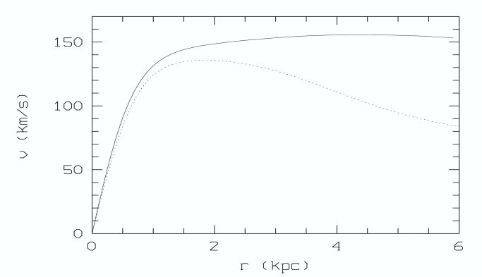
Figure 1: Rotation curve of the unperturbed potential. The dotted line represents the contribution of the disc.

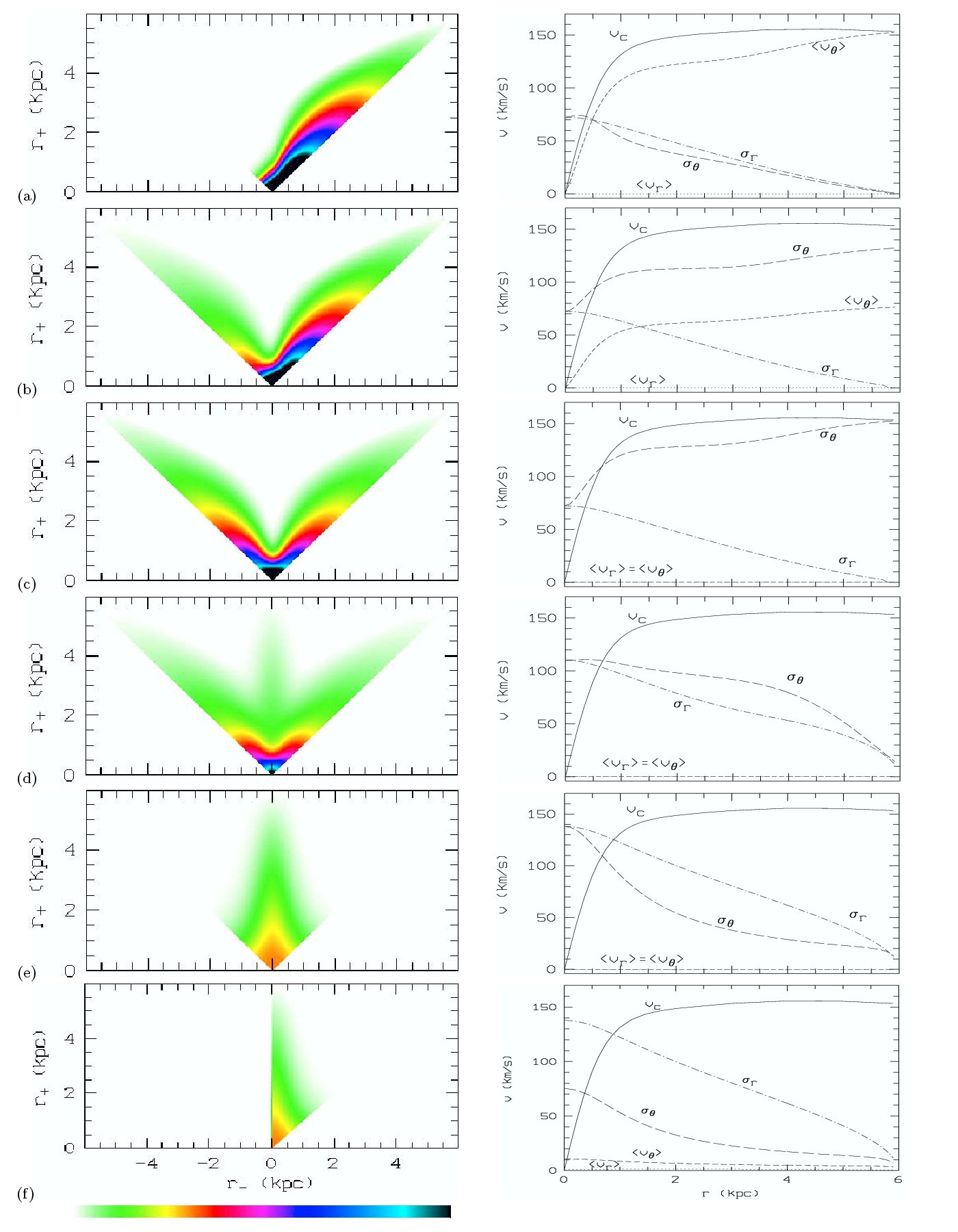
Figure 2: Unperturbed distribution functions (left) and unperturbed moments (right) of a few analysed models: (a) $f_{0}^{0,0}$, (b) $f_{0}^{0.25,0}$, (c) $f_{0}^{0.5,0}$, (d) $f_{0}^{0.5,0.5}$, (e) $f_{0}^{0.5,1}$, (f) $f_{0}^{0,1}$. For the distribution functions the density is decreasing linear from black to white.

A dynamical model for a disc galaxy embedded in a dark halo is specified by the global potential of the system and the distribution function of the stellar disc. For all the models that will be analysed in this paper, we have chosenb¿ the same unperturbed potential and unperturbed density but different distribution functions. The unperturbed potential in the plane of the disc is given by:

$$V_{0}(r)=\frac{GM}{\sqrt{1+r^{2}}}+\frac{GM}{\sqrt{1+(\frac{r}{4.4})^{2}}},$$ (13)

with $M=10^{10}M_{\odot}$ and $r$ expressed in kpc. This potential produces a rotation curve that rises near the centre and becomes flat further out in the disc, as can be seen in Fig. 1. For the unperturbed density profile we choose an approximately exponential profile:

$$\rho_{0}=\alpha e^{-1.3\sqrt{0.2+r^{2}}}.$$ (14)

The mass of the disc, and thus the mass of the halo, is determined by $\alpha$. We impose an outer limit at $r_{\rm max}=6$ kpc. We have chosen $\alpha$ so that the proportion $H/D$ of the total mass inside the outer radius $r_{\rm max}$ for the halo and the disc is about $2.5$. The disc is truncated by demanding that the distribution function $f_{0}(E,J)$ is zero for orbits that venture outside this outer limit. The distribution function is written as a linear combination of a basic set of distribution functions. The coefficients of this expansion are determined by a least-square fit to the density profile given by eq. (14). In all the models, the error on the fit to the mass density never exceeds $1\%$ of the central value. The contribution of the disc to the rotation curve is shown in Fig. 1.

We start with a strongly tangentially anisotropic model that is known to develop strong spiral arms (Vauterin & Dejonghe, 1996). Its distribution function $f_{0}^{0,0}(E,J)$ is shown in the left column of Fig. 2a. Most stars in this model populate nearly circular orbits that rotate in one direction. The unperturbed moments are shown in the right column of Fig. 2a. Using the distribution function $f_{0}^{1,0}(E,J)=f_{0}^{0,0}(E,-J)$, which has the same unperturbed density as $f_{0}^{0,0}(E,J)$, one can easily construct counter-rotating discs that all have the same density distribution. In order to place a fraction $x$ of all stars on retrograde orbits, the following distribution function can be used :

$$f_{0}^{x,0}(E,J)=(1-x)f_{0}^{0,0}(E,J)+xf_{0}^{1,0}(E,J).$$ (15)

In Fig. 2b, we plotted the distribution function and unperturbed moments of a model in which $25$ per cent of the stars counter-rotate. In Fig. 2c, we present the properties of a model consisting of two equally massive counter-rotating discs.

In the left column of Fig. 2e, we show the distribution function $f_{0}^{0.5,1}(E,J)$ of a very radially anisotropic model that is known to produce a strong bar instability (Vauterin & Dejonghe, 1996). Using this model we can construct models with varying degrees of radial anisotropy, as follows:

$$f_{0}^{0.5,y}(E,J)=(1-y)f_{0}^{0.5,0}(E,J)+yf_{0}^{0.5,1}(E,J).$$ (16)

In Fig. 2d, we plotted the properties of a model consisting of an even mix of $f_{0}^{0.5,0}$ and $f_{0}^{0.5,1}$ (i.e. $y=0.5$). We can also construct a similar family without counter-rotating discs:

$$f_{0}^{0,y}(E,J)=(1-y)f_{0}^{0,0}(E,J)+yf_{0}^{0,1}(E,J).$$ (17)

In Fig. 2f, we plotted the distribution function of $f_{0}^{0,1}$.

4 Lopsided instabilities

4.1 The influence of counter-rotation

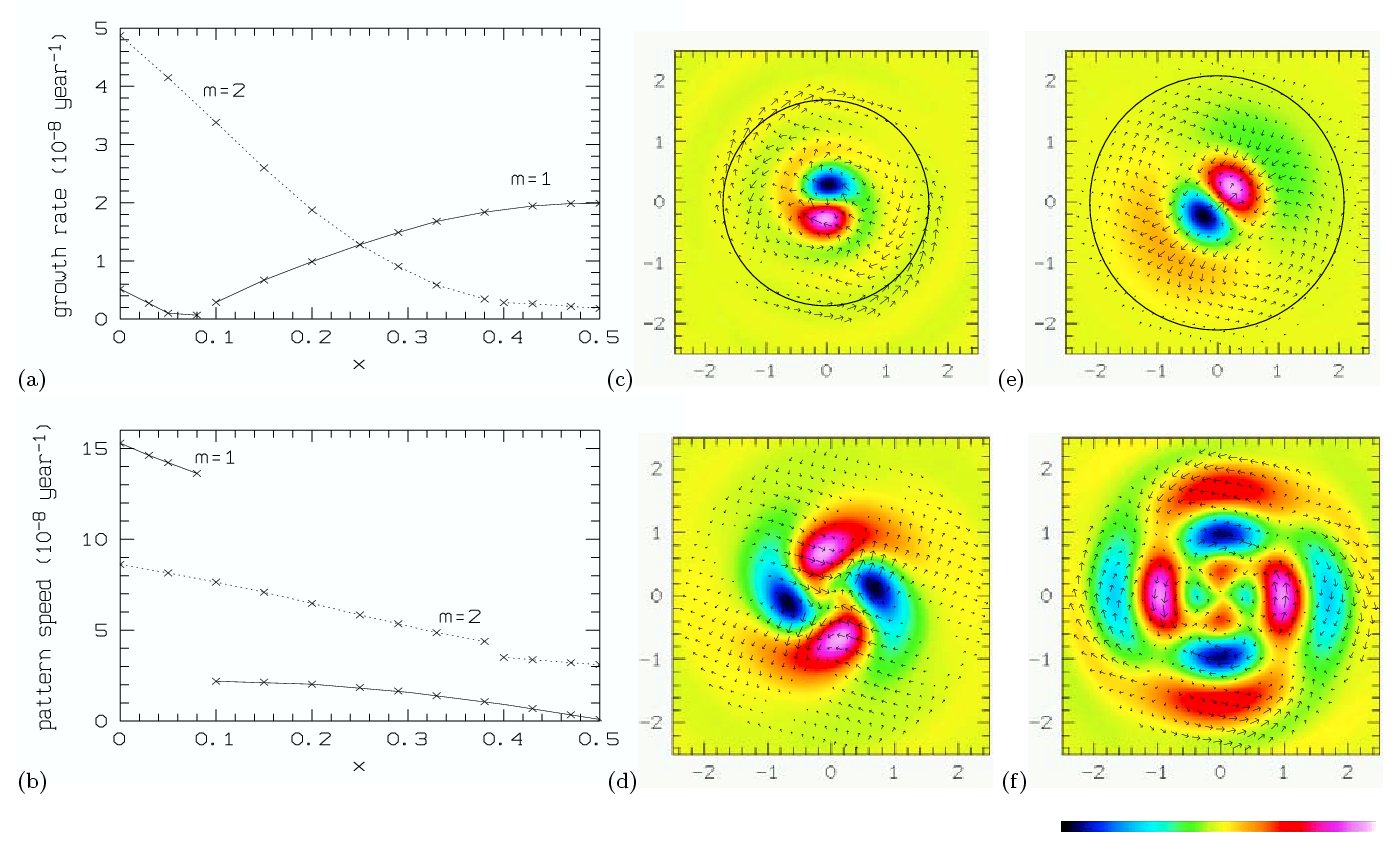
Figure 3: Growth rate (a) and pattern speed (b) for the strongest $m=1$ (solid line) and $m=2$ (dotted line) instabilities as the fraction $x$ of counter-rotating stars changes. Discontinuities appear when the nature of the instability changes. The perturbed density $\rho^{\prime}(\rho=\rho_{0}+\epsilon\rho^{\prime})$ and velocity field $\mathbf{v}^{\prime}(\mathbf{v}=\mathbf{v}_{0}+\epsilon\mathbf{v}^{\prime})$ is plotted out to a radius of $2.5$ kpc: (c) rotating one-armed spiral for $f_{0}^{0,0}$ , (d) rotating two-armed spiral for $f_{0}^{0,0}$, (e) non-rotating lopsided mode for $f_{0}^{0.5,0}$, (f) one of a pair of counter-rotating bars for $f_{0}^{0.5,0}$. Over-densities are coloured white-red, under-densities black-blue. In panels (c) and (e), we also indicate the radius within which a growing $m=1$ mode is expected based on density wave theory (see section 5 for a detailed discussion).

In Fig. 3, we show the growth rate and pattern speed of the fastest growing $m=1$ and $m=2$ modes as the fraction $x$ of counter-rotating stars for the models of the $f_{0}^{x,0}$ family changes. Clearly, the fully counter-rotating $f_{0}^{0.5,0}$ model has a dominant non-rotating $m=1$ instability whereas the $m=2$ instability is virtually absent (actually, two mirror-image $m=2$ modes with the same growth rates and opposite pattern speeds occur in the counter-rotating model). As the degree of counter-rotation diminishes, the growth rate of the $m=1$ instability slowly declines while it picks up a small pattern speed. At the same time, the $m=2$ instability increases in strength. As long as more than one quarter of all stars are on retrograde orbits, the model is dominated by a slowly rotating lopsided mode. Unexpectedly, around $x\approx 0.08$, the nature of the $m=1$ mode changes. Another, this time rapidly rotating, lopsided instability becomes the fastest growing $m=1$ mode. Its strength increases together with that of the $m=2$ mode as the degree of counter-rotation vanishes.

The dominant $m=1$ mode we find in strongly counter-rotating models is obviously the well-known counter-rotation instability. This instability has been known since Zang & Hohl (1978) and has been studied analytically (Sawamura, 1988; Palmer & Papaloizou, 1990; Tremaine, 2005) and using N-body simulations (Merritt & Stiavelli, 1990; Levison et al., 1990; Sellwood & Merritt, 1994; Sellwood & Valluri, 1997). Sellwood & Valluri (1997) do not detect it in systems rounder than E6, which is mainly the result of their rounder models being stabilised by a higher radial pressure. On the other hand, Merritt & Stiavelli (1990) find lopsidedness developing in systems as round as E1 but with negligible radial pressure. Partial rotation only introduces a pattern speed in an otherwise purely growing instability.

The counter-rotating bars we found, were also reported by Sellwood & Merritt (1994), Levison et al. (1990) and Friedli (1996). Sellwood & Valluri (1997) argued that they were the result of non-linear orbit trapping in finite-amplitude spiral disturbances. The fact that we found them shows that they are formed through linear instabilities.

Recently, some authors found a lopsided instability in a normal differentially rotating galactic disc (Saha, Combes & Jog, 2007). The lopsided pattern precesses in the disc with a very slow pattern speed with no preferred sense of precession. The weaker $m=1$ mode that we found in the rotating model has a certain sense of rotation and bears strong resemblance to the so-called eccentricity instability that occurs in gaseous and stellar near-Keplerian discs orbiting a central massive object (Adams, Ruden & Shu, 1989; Shu et al., 1990; Noh, Vishniac & Cochran, 1991; Taga & Iye, 1998; Lovelace et al., 1999; Jacobs & Sellwood, 2001; Bacon et al., 2001; Salow & Statler, 2004). Lovelace et al. (1999) constructed models for disc galaxies with exponentially declining surface density profiles embedded within a spherically symmetric dark halo. These authors found the inner regions of such systems rapidly develop a trailing one-armed spiral wave, even if the mass of the central object is small. The first N-body example of a rotating lopsided instability was found by Sellwood (1985) in a mass model of our Galaxy without a halo component. Evans & Read (1998) examined the global stability of stellar power-law discs. They report a similar rotating lopsided pattern in cut-out power-law discs, but found no growing non-axisymmetric modes in the fully self-consistent power-law discs. We provide the first theoretical evidence, based on a thorough mode-analysis of a suite of self-consistent dynamical models for disc galaxies embedded in a dark halo, that the eccentricity instability can also occur in the fully prograde stellar discs of spiral galaxies without an additional massive central component, such as a compact bulge or super-massive black hole, and without introducing an unresponsive central region in the disc.

4.2 Anisotropy

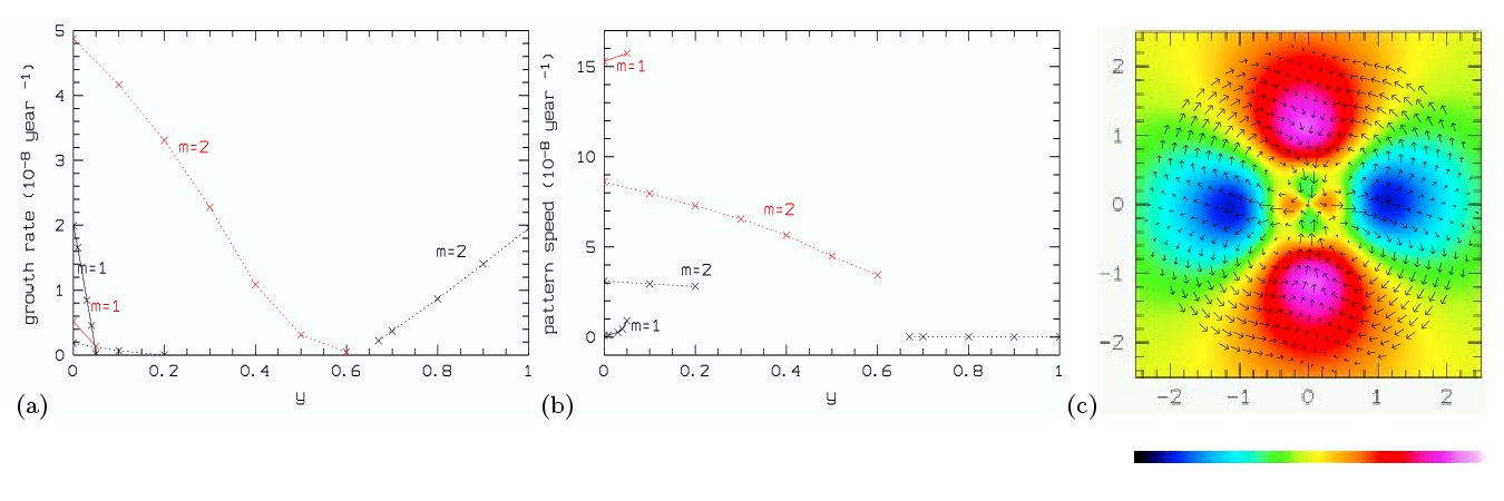
Figure 4: Growth rate (a) and pattern speed (b) for the strongest $m=1$ (solid line) and $m=2$ (dotted line) instabilities as the fraction $y$ of stars on radial orbits changes for the non-rotating (black) and rotating models (red). The perturbed density $\rho^{\prime}(\rho=\rho_{0}+\epsilon\rho^{\prime})$ and velocity field $\mathbf{v}^{\prime}(\mathbf{v}=\mathbf{v}_{0}+\epsilon\mathbf{v}^{\prime})$ is shown for model $f_{0}^{0.5,1}$ in (c). Over-densities are coloured white-red, under-densities black-blue.

We now study the behaviour of the self-consistent $m=1$ and $m=2$ as the fraction $y$ of stars on radial orbits changes. The variation of the growth rate and pattern speed is presented in Figs. 4a and 4b for the models $f_{0}^{0.5,y}$ (black) and $f_{0}^{0,y}$ (red). We start from model $f_{0}^{0.5,0}$ that is known to develop a strong non-rotating $m=1$ instability and two twin counter-rotating bar instabilities. As $y$, and thus the fraction of stars on radial orbits, increases, the $m=1$ and $m=2$ instabilities rapidly stabilise. The lopsided mode is the first to stabilise, at $y\approx 0.05$. The model becomes fully stable against both $m=1$ and $m=2$ modes at $y\approx 0.2$. For $y\gtrsim 0.6$, the model develops a non-rotating bar instability that becomes stronger as radial anisotropy increases. The perturbed density and velocity field of the bar of the $f_{0}^{0.5,1}$ are shown in Fig. 4c. If we start from model $f_{0}^{0,0}$, the $m=1$ and $m=2$ instabilities also stabilise with increasing anisotropy. The $m=2$ instability, is the last one to stabilise and the model becomes stable for $y\gtrsim 0.6$.

From this exercise, it is clear that the mechanism that is responsible for triggering the lopsided mode in the counter-rotating model relies heavily on virtually all stars moving on near-circular orbits. Even a relatively small contribution of stars on radial orbits makes it impossible for the disc to develop the $m=1$ mode.

4.3 Perturbed line-of-sight velocity fields

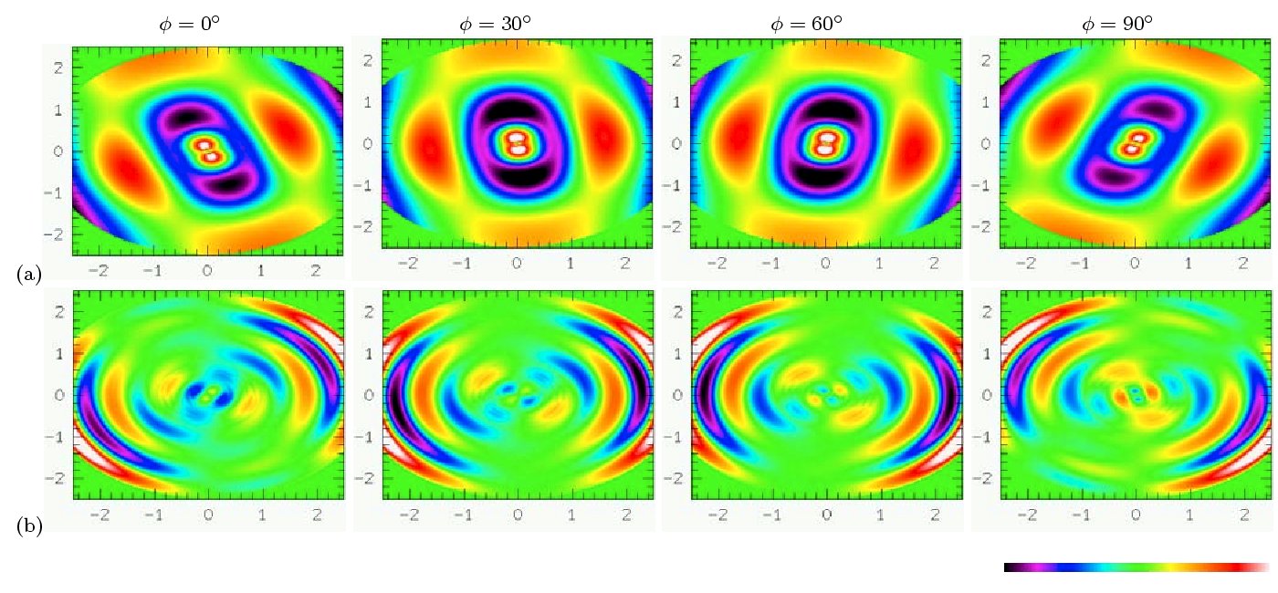
Figure 5: Residual line-of-sight velocity field $v_{\rm los}^{\prime}$ (with $v_{\rm los}=v_{\rm los,0}+\epsilon v_{\rm los}^{\prime})$ for the $m=1$ instabilities of (a) $f_{0}^{0.5,0}$ and (b) $f_{0}^{0,0}$ . All fields have an inclination of 50^∘ and a viewing angle $\phi$ varying from 0^∘ to 90^∘ in steps of 30^∘. Positive velocities are coloured white-red, negative velocities black-blue.

To allow for a direct comparison of our models with observations, we present in Fig. 5 the perturbed line-of-sight velocity fields for the extreme cases of exact counter-rotation (top row) and full prograde rotation (bottom row). The first-order perturbation to the velocity $\mathbf{v}^{\prime}$, corresponding to the perturbation $f^{\prime}$ to the distribution function $f_{0}$, is given by

$$\mathbf{v}^{\prime}=\frac{\int\mathbf{v}f^{\prime}{\rm d}\mathbf{v}-\rho^{\prime}\mathbf{v}_{0}}{\rho_{0}}$$ (18)

This velocity perturbation is then projected onto the sky in order to obtain the perturbation on the line-of-sight velocity, denoted by $v_{\rm los}^{\prime}$. The velocity fields in Fig. 5 have an inclination $i=50^{\circ}$ and a viewing angle $\phi$ ranging from $0^{\circ}$ to $90^{\circ}$. The velocity fields are only plotted out to a radius of 2.5 kpc since only inside this region is the density perturbation noticeable. Schoenmakers et al. (1997) showed that if the potential contains a perturbation of harmonic number $m$ then the line-of-sight velocity field contains $n=m-1$ and $n=m+1$ terms. Thus as expected, we can see $n=0$ and $n=2$ components in the residual velocity fields but there is no strong direct resemblance with the two galaxies discussed by Swaters et al. (1999), one of which shows a dominant $n=2$ velocity perturbation while the other exhibits predominantly a $n=0$ structure. Of course, the residual velocity fields plotted in Fig. 5 are calculated using linear perturbation theory. Instabilities in real galaxies are likely to be in the non-linear regime. Therefore, this comparision is intended to be indicative not definitive.

5 Physical interpretation

In order to unravel the physics behind the two distinct $m=1$ modes found in section 4, we will study the orbits of stars that move in the global perturbed potential:

$$V(r,\theta,t)=V_{0}(r)+\epsilon V^{\prime}(r)e^{i(m\theta-\omega t)}.$$ (19)

In order to simplify the interpretation, we keep the amplitude of the perturbation fixed, i.e. we set $\Im(\omega)=0$, and only consider its pattern speed, $\Re(\omega)/m$. The prefactor $\epsilon$ is determined by requiring that the maximum difference between the perturbed and the unperturbed density nowhere exceeds 10 % of the unperturbed density. We then numerically evolve an ensemble of stars in the perturbed potential using a leapfrog integrator. The goal is to see how the orbits are affected by the perturbation and which perturbed orbits help support the perturbation. For brevity, we will henceforth refer to the $m=1$ instability of the $f_{0}^{0.5,0}$ model as the “non-rotating lopsided mode”, and to that of the $f_{0}^{0,0}$ model as the “rotating lopsided mode”.

5.1 Non-rotating lopsided mode

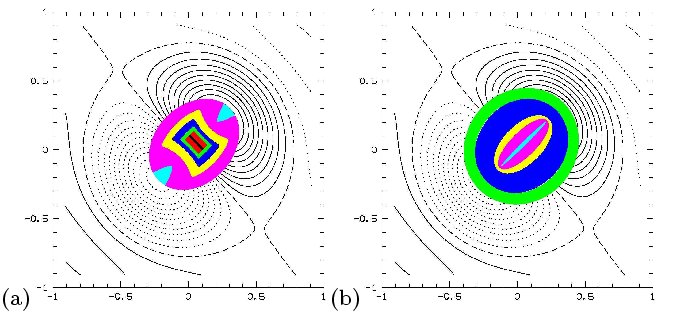
Figure 6: Stellar orbits in the potential well of the non-rotating lopsided mode. All orbits have the same energy but different angular momentum: Angular momentum increases in figure (a) from the black orbit ($J=0$) to the cyan orbit ($J=J_{c}$) and in figure (b) from the cyan orbit ($J=J_{c}$) to the green orbit ($J=1.9~{}J_{c}$).

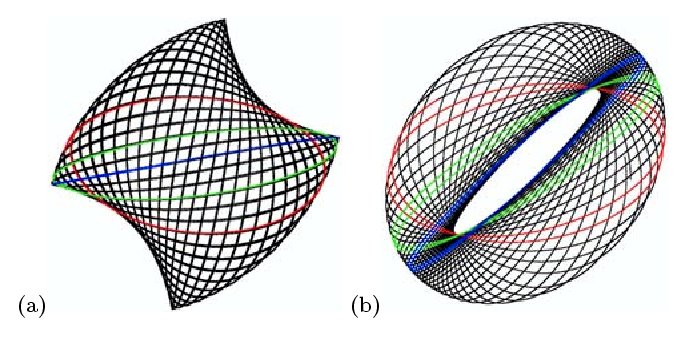
Figure 7: (a) Butterfly orbit. (b) Loop orbit. To see the evolution in time, we indicated some parts of the orbit in colour. The first part red, the second part green and the last part blue.

In Fig. 6, we present some perturbed stellar orbits that occupy the region in which the density perturbation is maximal. They all share the same energy but are characterised by a different angular momentum. We can easily recognise two general orbit families : butterflies and loops. In Fig. 7a we show a more detailed picture of a butterfly orbit. A butterfly can be viewed as a librating elliptical orbit with variable eccentricity. At the turning points of the libration, the orbit ellipticity becomes zero (this is evidenced by the red, green, and blue ellipses in Fig. 7a). As the angular momentum of the orbit is increased up to a critical point $J_{c}$, the two instances of zero ellipse orbit ellipticity coincide and the orbit fills an elliptical region. For still higher angular momentum, libration becomes rotation and the orbit becomes a loop, as can be seen in Fig. 6b & Fig. 7b. Remarkably, both orbit families are also found by Jalali & Rafiee (2000) for a disc galaxy model with a lopsided potential that is of Stäckel form in elliptic coordinates and with two separate strong density cusps. They also found two other orbit families, nucleophilic bananas and horseshoe orbits. It is clear from their formulation that these two orbit families are associated with the cusps having diverging central densities which is why we do not find them in our models.

5.1.1 Linear regime

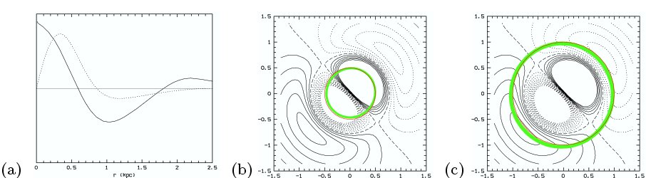
Figure 8: (a) The sign of the quantity $C_{2}(r)$ (solid line) roughly traces that of the density perturbation (dotted line). Perturbed orbits (green) are displaced from the unperturbed orbit (red orbit): orbits with $C_{2}>0$ are shifted into the direction of the overdensity (b), those with $C_{2}<0$ are shifted into the opposite direction (c).

The mechanism that causes the non-rotating $m=1$ mode is now clear : an infinitesimal $m=1$ perturbation will cause near-circular orbits to become somewhat more elliptic and to shift towards the slight overdensity, thus adding to this over-density, which in turn causes other orbits to become more elongated and to shift, and so on. This was already evident from section 3.3 3(a) of Binney & Tremaine (1987) who used perturbation theory in combination with the epicyclic approximation to calculate the response of near-circular orbits to a general $m$-armed perturbation. Since this perturbation has no Lindblad resonances, the condition that the sign of the quantity $C_{2}(r)=dV^{\prime}(r)/dr+2V^{\prime}(r)/r$ (represented by the red curve in Fig. 8a) traces that of the orbit displacement is fulfilled everywhere within the stellar disc (see eq. (3-120b) of Binney & Tremaine (1987)) and the perturbed near-circular orbits will all strengthen the $m=1$ mode. Tangential orbits with $C_{2}>0$ are shifted into the direction of the overdensity (Fig. 8b), those with $C_{2}<0$ are shifted into the opposite direction (Fig. 8c). As a consequence, the sign $C_{2}$ also roughly follows that of the density perturbation.

With a maximum density contrast of 10%, the orbits plotted in Figs. 6 and 7 are not per se in the linear regime. This was done, since we here only wish to illustrate the mechanism that induces the instability to grow, for clarity : a truly infinitesimal perturbation would result in an equally infinitesimal and therefore nearly invisible shift of the tangential orbits.

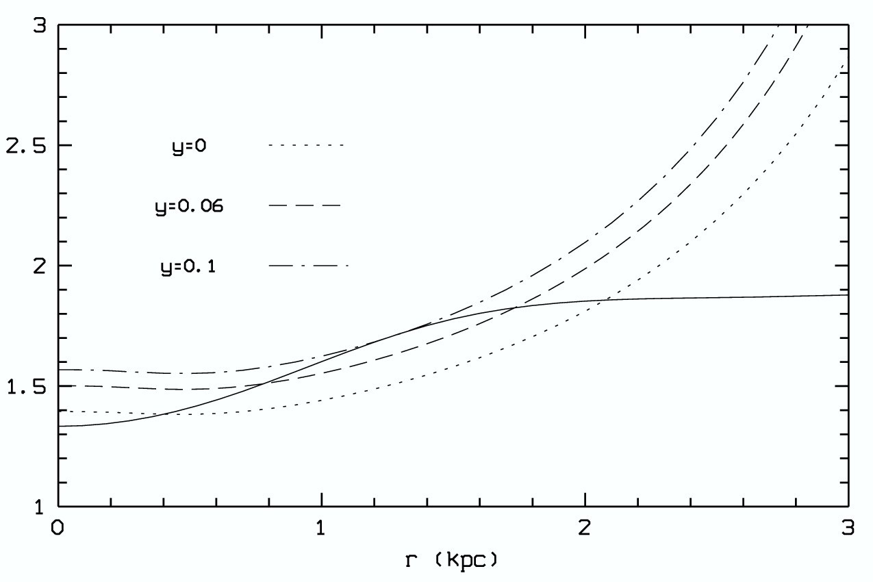
Figure 9: In a counter-rotating disc, purely growing WKB waves may develop when $Q(r)$ (dashed line) $\leq\frac{\kappa(r)^{2}}{\kappa(r)^{2}-\Omega(r)^{2}}$ (solid line). The quantity $\frac{\kappa(r)^{2}}{\kappa(r)^{2}-\Omega(r)^{2}}$ is plotted using a full line. The $Q-$ profiles of several counter-rotating models, with increasing radial anisotropy as quantified by the parameter $y$ in eq. (16), are overplotted (see legend in the figure). Models with $y\gtrsim 0.06$ are stable, both according to Palmer’s stability criterion and our mode analysis.

It is instructive to interpret this instability not only on the level of stellar orbits but also in terms of density waves. As shown in Palmer’s book on dynamical instabilities (Palmer, 1994), a razor-thin disc consisting of two equal-mass counter-rotating stellar populations may develop purely growing one-armed ($m=1$) WKB waves if the Toomre parameter, $Q=\frac{\sigma_{r}\kappa}{3.36G\rho_{0}}$, fails to satisfy the local stability criterion

$$Q(r)\geq\frac{\kappa(r)^{2}}{\kappa(r)^{2}-\Omega(r)^{2}}.$$ (20)

This is very similar to the well-known criterion $Q\geq 1$ for local stability against purely growing $m=0$ waves. The precise form of this stability criterion depends on three approximations, (i) the WKB approximation for tightly wound spiral waves, (ii) the epicycle description for near-circular stellar orbits, and (iii) a Gaussian distribution function. None of these necessarily applies to the models presented in this paper. Nonetheless, we used the $Q(r)$, $\kappa(r)$, and $\Omega(r)$ profiles of the fully counter-rotating $f_{0}^{0.5,y}$ models to evaluate this criterion as a function of radius, where $Q$ depends on the parameter $y$ via the radial velocity dispersion (Fig. 9). We only check the fully counter-rotating models since only in this case can an analytical stability criterion be derived. It is clear from Figs. 3(e) & 9 that the region where, according to the local stability criterion, purely growing waves may develop roughly coincides with the region in which the non-rotating lopsided mode resides (i.e. inside a radius $r\lesssim 2.1$ kpc).

As a further test, we checked whether the model that, according to our mode-analysis, is the first to be stabilized by increasing radial anistropy, is also stable according to Palmer’s criterion. This is done by increasing the parameter $y$ in eq. (16). It is clear from Fig. 9 that the $Q(r)$ profile of the first stable model according to our mode-analysis, the one with $y\approx 0.06$ (see fig. 4a), is also very close to the line of stability according to Palmer’s criterion. For $y\geq 0.1$, the models are definitely stable both according to Palmer’s criterion and our mode-analysis. Note that Palmer’s stability criterion is a sufficient one : satisfying it implies stability, not satisfying it does not necessarily imply instability. Given the reasonable agreement between Palmer’s analysis and our mode analysis concerning the line of stability and the spatial extent of the $m=1$ pattern, we are led to the conclusion that the purely growing lopsided mode we find in counter-rotating discs is caused by a local Jeans-type instability.

5.1.2 Non-linear regime

Figs. 6 and 7 reveal a feature that is not captured by our linear mode-analysis. Once the perturbation is strong enough, radial orbits are deformed into the new family of butterfly orbits whose centres of gravity are also shifted in the direction of the over-density. Thus, this orbit family may potentially contribute to the $m=1$ perturbation but only after the amplitude of the perturbation has become large enough, see also Jalali & Rafiee (2000). For an infinitesimal perturbation, radial orbits do not contribute to the growth of the instability (their presence is even detrimental to the instability’s growth in the linear regime, see below).

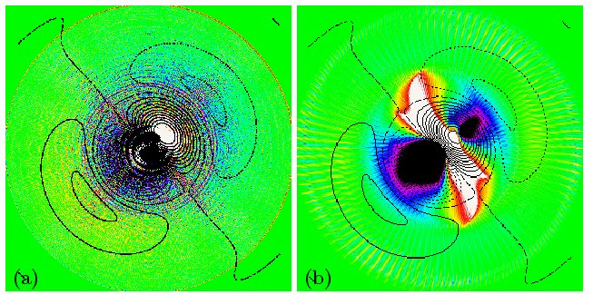
Figure 10: The change in the density distribution of an ensemble of orbits, $\delta\!\rho$, as defined by eq. (21), due to the non-rotating $m=1$ mode. Panel (a) : an ensemble of circular unperturbed orbits; panel (b) : an ensemble of radial unperturbed orbits. Negative values of $\delta\!\rho$ are coloured black/blue; positive values in white/yellow. The contours of the perturbed density of the $m=1$ mode are also plotted (solid line: over-density, dotted line: under-density). See text for a discussion of this figure.

Further evidence for this mechanism can be gleaned from the following exercise. A test particle with initial conditions $(\mathbf{r}_{0},\mathbf{v}_{0})$ on an orbit in the unperturbed system with potential $V_{0}(r)$ over time fills a certain area, which, in general will have the form of an annulus (with circular and straight-line orbits as extremes). For the same initial conditions $(\mathbf{r}_{0},\mathbf{v}_{0})$, the test particle’s orbit in the perturbed potential $V(r)$ will fill a differently shaped area. The difference between the density distribution of the perturbed orbit and that of the unperturbed orbit gives an idea of how the density of a galaxy made up of an ensemble of unperturbed orbits will change under the influence of the given perturbation. In Fig. 10, we show how the density distribution of an ensemble of circular orbits (10a) or radial orbits (10b) changes due to the perturbation given by eq. (19); i.e., we plot the quantity

$$\delta\!\rho(r,\theta)=\sum_{\rm orbit}\left(\rho_{\rm orbit,pert}(r,\theta)-\rho_{\rm orbit,unpert}(r,\theta)\right)$$ (21)

where the sum runs over an ensemble of circular unperturbed orbits with different radii and with the phases of the starting points of the orbit integrations distributed uniformly over the interval [0,2$\pi$[ (circles in Fig. 10a and spokes in Fig. 10b are caused by the finite number of orbits). Negative values of $\delta\!\rho$ are coloured black/blue; positive values in white/yellow. Clearly, the regions where $\delta\!\rho>0$ coincide with the over-densities of the $m=1$ mode (full line contours) whereas the regions where $\delta\!\rho<0$ coincide with the mode’s under-densities (dotted line contours). It is obvious from Fig. 10b that the radial orbits are not nearly as cooperative despite the fact that they are slightly displaced towards the inner overdensity. As an ensemble, they do not react to the imposed perturbation in a way that would tend to strengthen it since their long axes are oriented perpendicularly to the inner lopsidedness leading rather to a $m=2$ feature. The (near-)circular orbits are clearly the backbone of this $m=1$ mode and, as we know from Fig. 4a, even a smidgen of stars on radial orbits is enough to stabilise the system against this instability.

5.2 Rotating lopsided mode

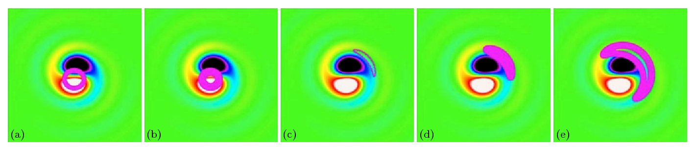
Figure 11: Stellar orbits in the force field of the rotating lopsided mode, as seen in a reference frame rotating with the same pattern speed as the lopsided mode. We find two orbit families : (a) & (b) loop orbits, and (c), (d) & (e) banana orbits.

In Fig. 11, we present five perturbed stellar orbits that occupy the region in which the density perturbation due to the rotating lopsided mode is maximal. The orbits are plotted in a reference frame that rotates with the pattern speed of the $m=1$ mode. Again we observe loop orbits that are displaced into the direction of the over-density and that can support the lopsided structure (Fig. 11a & 11b). At larger radii, the stellar orbits attain a banana shape in this reference frame. These orbits occupy a region outside the mode’s main under-density and seem to be connected to the one-armed spiral (Fig. 11c, 11d & 11e). Unlike in the previous case, where aligned loop orbits were almost solely responsible for creating the instability, here the two orbit families fulfil different tasks. The aligned loop orbits support the inner lobes of the lopsided structure whereas the banana orbits make up the outer one-armed spiral.

5.2.1 Linear regime

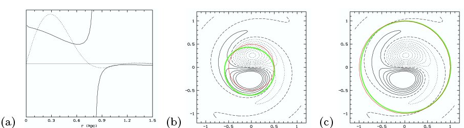
Figure 12: (a) The sign of the quantity $C_{2}(r)$ (solid line) roughly traces that of the density perturbation (dotted line). Perturbed orbits (green) are displaced from the unperturbed orbit (red orbit). Orbits with $C_{2}>0$ are shifted into the direction of the overdensity (b) and those with $C_{2}<0$ are shifted into the opposite direction (c).

For the lopsided mode with pattern speed $\Omega_{p}$, the quantity $C_{2}(r)$ from Binney & Tremaine (1987) becomes:

$$C_{2}(r)=\frac{1}{\kappa^{2}-m^{2}(\Omega-\Omega_{p})^{2}}\left(\frac{{\rm d}V^{\prime}(r)}{{\rm d}r}+2\frac{\Omega V^{\prime}(r)}{r(\Omega-\Omega_{p})}\right).$$ (22)

The sign of $C_{2}$ again traces that of the orbit displacement and, with less fidelity, of the density perturbation (Fig. 12a). Orbits inside the corotation radius are shifted into the direction of the overdensity $(C_{2}>0)$ (Fig. 12b). At corotation, $C_{2}$ diverges. Orbits near corotation become banana orbits. The corotation radius of the mode is at $r_{c}=0.8$ kpc, which coincides with the position of the one-armed spiral. Outside corotation, the sign of $C_{2}$ changes and orbits are shifted into the other direction (Fig. 12c).

The interpretation of this instability in terms of waves is somewhat subtle. In the case of a bar instability, the radial extent of the $m=2$ pattern is determined by the largest radius out to which the most slowly rotating wave that avoids having an inner Lindblad resonance (ILR) can travel. This constraint sets the size of the resonance cavity within which the pattern can grow by swing amplification. However, one-armed waves do not have an ILR, irrespective of their pattern speed. The radial extent of the $m=1$ pattern is set by the largest radius out to which non-rotating wave packets can travel. This radius is determined by the disc’s dispersion relation. We used the WKB dispersion relation (eq. (6-46) of Binney & Tremaine (1987) or eq. (12.82) of Palmer (1994)) together with the $Q(r)$, $\kappa(r)$, and $\Omega(r)$ profiles of the $f_{0}^{0,0}$ model to estimate the region in which non-rotating one-armed waves are allowed to exist. The $Q(r)$ profile of the fully rotating $f_{0}^{0,0}$ model rises outwardly, limiting the extent of non-rotating waves to some finite radius, well within the disc. In the case of the $f_{0}^{0,0}$ model, for a zero pattern speed, the dispersion relation has two branches (the long-wave and the short-wave branch) of incoming and outgoing leading and trailing waves for radii smaller than approximately 1.7 kpc. This sets the dimension of the resonance cavity within which the pattern can grow through swing amplification. All $m=1$ waves can propagate into the galaxy center where incoming trailing wave packets are reflected as outgoing leading wave packets, closing the feedback loop. Moreover, a more steeply rising rotation curve will suppress the $m=2$ mode while leaving the $m=1$ mode, which has no inner Lindblad resonance, largely intact.

Thus, following Evans & Read (1998) who already proposed this mechanism as the cause of the $m=1$ modes found in cut-out power-law discs, we propose swing amplification as the physical cause of the one-armed mode in this rotating model.

5.2.2 Non-linear regime

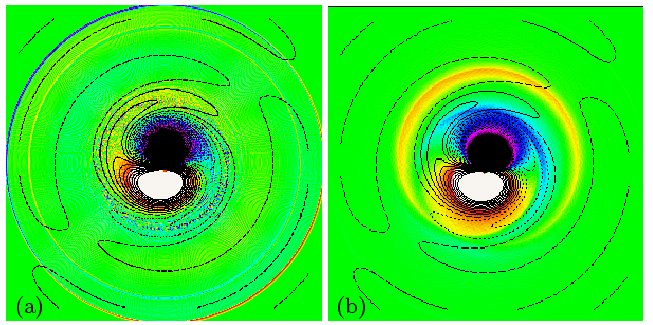
Figure 13: The change in the density distribution due to the rotating $m=1$ mode. Panel (a) : an ensemble of circular unperturbed orbits; panel (b) : an ensemble of radial unperturbed orbits. Negative values are coloured black/blue; positive values in white/yellow. The contours of the perturbed density of the $m=1$ mode are also plotted (solid line: over-density, dotted line: under-density)

[width=17cm]

In Fig. 13, we show how the density distribution, i.e. the quantity $\delta\!\rho$, defined by eq. (21), of an ensemble of circular (panel (a)) and of radial (panel (b)) orbits changes due to the rotating $m=1$ mode. We now see that the circular orbits and the radial orbits both support the lopsided structure. This is because radial orbits as well as the inner circular orbits become loop orbits that are aligned with the lopsided mode. If we change the fraction of stars on radial orbits, we have a slower stabilisation of the $m=1$ mode than in the non-rotating models (see Fig. 4a).

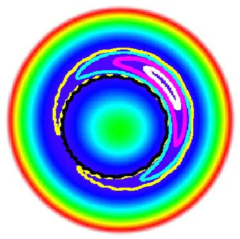
Figure 14: A few banana orbits in a frame rotating with the lopsided mode. All orbits start from co-rotation with the same energy and angular momentum, but at a different angle $\theta$: white ($\theta=45^{\circ}$), purple ($\theta=90^{\circ}$), cyan ($\theta=135^{\circ}$), yellow ($\theta=180^{\circ}$), black ($\theta=225^{\circ}$). The effective potential is also shown (increasing from white to blue).

We have integrated a number of stellar orbits that all start at the corotation radius $r=r_{c}$ with phases $\theta=45^{\circ},\,90^{\circ},...225^{\circ}$. The results are shown in Fig. 14 where we also showed the effective potential

$$V_{\rm eff}(r,\theta)=V(r,\theta)-\frac{1}{2}\left(\Im(\omega)\right)^{2}r^{2}.$$ (23)

All banana orbits evolve around the stable Lagrange point of the system which is located at the local maximum of the effective potential at a phase angle $\theta_{L}$. In the corotating reference frame, a star at position ($r_{c},\theta_{L}$) will remain there forever. Orbits started at corotation but with different phase angles will trace out a banana-shaped curve. The further away from the equilibrium point $(r_{c},\theta_{L})$ an orbit is started, the more elongated the banana becomes. The orbit started at $(r_{c},180^{\circ}+\theta_{L})$ is circular in the corotating reference frame. The origin of the one-armed spiral now becomes more clear. A weak, rotating lopsided perturbation will catch stars close to the ($r_{c},\theta_{L}$) Lagrange point on banana orbits. These then spend more time near the stable Lagrange point, creating an over-density there, and less time near the diametrically opposite point, creating an under-density there. Thus, the banana orbits help strengthen the lopsided mode, causing more stars to be trapped in banana orbits, and so on.

6 conclusions

Using a toy dynamical model, we have investigated the properties and causes of dynamical instabilities that may cause lopsidedness in disc galaxies.

We found the well-known counter-rotation instability to be the dominant mode in disc galaxy models with strong counter-rotation and small radial anisotropy. It is much stronger than any $m=2$ mode we found in these models. The strength of this mode diminishes in models with less counter-rotation and it eventually disappears in fully rotating models. These, however, develop a different type of lopsided mode, that becomes stronger as rotation increases, although it is always much weaker than the $m=2$ spiral-arm mode. This instability bears strong resemblance to the eccentricity instability that is known to occur in gaseous and stellar near-Keplerian discs orbiting a central massive object. We provide the first theoretical evidence, based on a thorough mode-analysis of a suite of dynamical models for disc galaxies embedded in a dark halo, that the eccentricity instability can also occur in the fully pro-grade stellar discs of spiral galaxies.

By integrating the orbits of an ensemble of stars in the perturbed potential of the two extreme cases of full counter-rotation on the one hand and full prograde rotation on the other hand, we investigated the physics underlying the counter-rotation and eccentricity instability. The counter-rotation instability grows by changing near-circular orbits into aligned loop orbits that help maintain a lopsided structure. If the non-linear regime, radial orbits are changed into butterfly orbits. In the case of the eccentricity mode, both radial and tangential orbits become aligned loops in a corotating reference frame. In the non-linear regime, orbits near corotation are trapped into resonance and describe banana-shaped figures in a corotating frame. They help support the characteristic one-armed spiral.

In terms of density waves, the counter-rotating $m=1$ mode is most likely due to a purely growing Jeans-type instability. An approximative analytical criterion for local stability, akin to Toomre’s stability criterion for axisymmetric waves, can be employed to estimate the region in which purely growing one-armed waves may develop. This estimate roughly coincides with the region in which the non-rotating lopsided mode is observed to reside. The rotating $m=1$ mode, on the other hand, grows as a result of the swing amplifier working inside the resonance cavity that extends from the disc center out to the radius where non-rotating rotating waves are stabilized by the model’s outwardly rising $Q$-profile. Rotating waves are confined to even smaller radii so the non-rotating waves effectively set the outer boundary of the resonance cavity.

Many disc galaxies show a noticeable $m=1$ perturbation besides the dominant $m=2$ spiral-arm mode but only very few of them show any counter-rotation. The rotating lopsided mode we identified in fully prograde disc models therefore forms an attractive explanation for this observed phenomenon.

References

- Adams, Ruden & Shu (1989) Adams F. C., Ruden S. P., Shu F. H., 1989, ApJ, 347, 959
- Angiras et al. (2006) Angiras R. A., Jog C. A., Omar A., Dwarakanath K. S., 2006, MNRAS, 369, 1849
- Bacon et al. (2001) Bacon R., Emsellem E., Combes F., Copin Y., Monnet G., Martin P., 2001, A&A, 371, 409
- Bertola & Corsini (1999) Bertola F., Corsini E.M., 1999, in Galaxy Interactions at Low and High Redshift, ed. J. E. Barnes & D. B. Sanders, IAUSymp., 186, 149
- Binggeli et al. (2000) Binggeli B., Barazza F., Jerjen H., 2000, A&A, 359, 447
- Binney & Tremaine (1987) Binney, J. & Tremaine, S., 1987, “Galactic Dynamics”, Princeton Univ. Press, Princeton, New Jersey, US
- Bournaud et al. (2005) Bournaud F., Combes F., Jog C. J., Puerari I., 2005, A&A, 438, 507
- Côté et al. (2006) Côté P. et al, 2006, ApJS, 165, 57
- De Rijcke & Debattista (2004) De Rijcke S., Debattista V.P., 2004, ApJ, 603, L25
- Evans & Read (1998) Evans N. W. & Read J. C. A., 1998, MNRAS, 300, 106
- Friedli (1996) Friedli D., 1996, A&A, 312, 761
- Haynes et al. (1998) Haynes M. P., Hogg D. E., Maddalena R. J., Roberts M. S., van Zee L., 1998, AJ, 304, 62
- Jacobs & Sellwood (2001) Jacobs V. & Sellwood, J. A., 2001, ApJ, 555, L25
- Jalali & Rafiee (2000) Jalali M. A., Rafiee A. R., 2000, MNRAS, 320, 379
- Jog (1997) Jog C. J., 1997, ApJ, 448, 642
- Jog (1999) Jog C. J., 1999, ApJ, 522, 661
- Kalnajs (1977) Kalnajs A. J., 1977, ApJ, 212, 637
- Kannappan & Fabricant (2001) Kannappan S. J. & Fabricant D. G., 2001, AJ, 121, 140
- Kuijken et al. (1996) Kuijken K., Fisher D., Merrifield M. R., 1996, MNRAS, 283, 543
- Levine & Sparke (1998) Levine S. E. & Sparke L. S., 1998, ApJ, 496, L13
- Levison et al. (1990) Levison H. F., Duncan M. J., Smith B. F., 1990, ApJ, 363, 66
- Lovelace et al. (1999) Lovelace R. V. E., Zhang L., Kornreich D. A., Haynes M. P., 1999, ApJ, 524, 634
- Merrifield and Kuijken (1994) Merrifield M. R., Kuijken K., 1994, ApJ, 432, 575
- Merritt & Stiavelli (1990) Merritt D. & Stiavelli M., 1990, ApJ, 358, 399
- Noh, Vishniac & Cochran (1991) Noh H., Vishniac E. T., Cochran W. D., 1991, ApJ, 383, 372
- Palmer (1994) Palmer P. L., 1994, “Stability of collisionless stellar systems”, Kluwer Academic Publishers, Dordrecht
- Palmer & Papaloizou (1990) Palmer P. L. & Papaloizou J., 1990, MNRAS, 243, 263
- Richter & Sancisi (1994) Richter O.-G., Sancisi R., 1994, A&A, 304, L9
- Rubin et al. (1992) Rubin V. C., Graham J. A., Kenney J. D. P. 1992, ApJ, 394, L9
- Saha, Combes & Jog (2007) Saha K., Combes F., Jog C.J. , 2007, eprint arXiv:0708.2873
- Salow & Statler (2004) Salow R. M., Statler T. S., 2004, ApJ, 611, 245
- Sawamura (1988) Sawamura M., 1988, PASJ, 40, 279
- Schoenmakers et al. (1997) Schoenmakers R. H. M., Franx M., de Zeeuw P. T. 1997, MNRAS, 292, 349
- Sellwood (1985) Sellwood J. A., 1985, MNRAS, 217, 127
- Sellwood & Merritt (1994) Sellwood J. A., Merritt D., 1994, ApJ, 425, 530
- Sellwood & Valluri (1997) Sellwood J. A., Valluri M., 1997, MNRAS, 287, 124
- Shu et al. (1990) Shu F. H., Tremaine S., Adams F. C., Ruden S. P., 1990, ApJ, 358, 495
- Swaters et al. (1999) Swaters R.A., Schoenmakers R. H., Sancisi R., van Albada T. S., 1999, MNRAS, 304, 330
- Taga & Iye (1998) Taga M. & Iye M., 1998, MNRAS, 299, 1132
- Tremaine & Yu (2000) Tremaine S. & Yu, Q., 2000, MNRAS, 319, 1
- Tremaine (2005) Tremaine S., 2005, ApJ, 625, 143
- Vauterin & Dejonghe (1996) Vauterin P., Dejonghe H., 1996, A&A, 313, 465
- Vergani et al. (2007) Vergani D., Pizzella A., Corsini E. M., van Driel W., Buson L. M., Dettmar R.-J., Bertola F., 2007, A&A, 463, 883
- Zang & Hohl (1978) Zang T. A. & Hohl F., 1978, ApJ, 226, 52