$\psi(2S)$ Radiative Decay Measurements

Abstract

Using a sample of 14 million $\psi(2S)$ events collected with the BESII detector, branching fractions or upper limits on the branching fractions of $\psi(2S)$ decays into $\gamma p\overline{p}$, $\gamma 2(\pi^{+}\pi^{-})$, $\gamma K^{0}_{S}K^{+}\pi^{-}+c.c.$, $\gamma K^{+}K^{-}\pi^{+}\pi^{-}$, $\gamma K^{\ast 0}K^{-}\pi^{+}+c.c.$, $\gamma K^{\ast 0}\overline{K}^{\ast 0}$, $\gamma\pi^{+}\pi^{-}p\overline{p}$, $\gamma 2(K^{+}K^{-})$, $\gamma 3(\pi^{+}\pi^{-})$ and $\gamma 2(\pi^{+}\pi^{-})K^{+}K^{-}$ with hadron invariant mass less than 2.9$~{}\mbox{GeV}/c^{2}$ are reported. We also report branching fractions of $\psi(2S)$ decays into $\gamma p\overline{p}\pi^{0}$, $p\overline{p}\pi^{0}\pi^{0}$, $2(\pi^{+}\pi^{-})\pi^{0}$, $\omega\pi^{+}\pi^{-}$, $\omega f_{2}(1270)$, $b_{1}^{\pm}\pi^{\mp}$ , $\pi^{0}K^{0}_{S}K^{+}\pi^{-}+c.c.$, $K^{\pm}\rho^{\mp}K^{0}_{S}$, $\pi^{0}2(\pi^{+}\pi^{-})K^{+}K^{-}$ and $\gamma\pi^{0}2(\pi^{+}\pi^{-})K^{+}K^{-}$.

I Introduction

Besides the conventional meson and baryon states, QCD (Quantum Chromodynamics) also predicts a rich spectrum of so-called QCD exotics, among them glueballs ($gg$), hybrids ($q\bar{q}g$), and four-quark states ($qq\bar{q}\bar{q}$) in the 1.0 to 2.5 $~{}\mbox{GeV}/c^{2}$ mass region. Therefore, the search for evidence of these exotic states plays an important role in testing QCD. Radiative decays of quarkonium are expected to be a good place to look for glueballs, and there have been many studies performed in $J/\psi$ radiative decays Jdecay ; QWG , while such studies have been limited in $\psi(2S)$ radiative decays due to low statistics in previous experiments PDG ; QWG . Radiative decays of $\psi(2S)$ to light hadrons are expected at about 1% of its total decay width PRD-wangp . However, the previously measured channels only sum up to 0.05% PDG .

In this paper we present measurements of $\psi(2S)$ decays into $\gamma p\overline{p}$, $\gamma 2(\pi^{+}\pi^{-})$, $\gamma K^{0}_{S}K^{+}\pi^{-}+c.c.$, $\gamma K^{+}K^{-}\pi^{+}\pi^{-}$, $\gamma K^{\ast 0}K^{-}\pi^{+}+c.c.$, $\gamma K^{\ast 0}\overline{K}^{\ast 0}$, $\gamma\pi^{+}\pi^{-}p\overline{p}$, $\gamma 2(K^{+}K^{-})$, $\gamma 3(\pi^{+}\pi^{-})$ and $\gamma 2(\pi^{+}\pi^{-})K^{+}K^{-}$ with the invariant mass of the hadrons ($m_{hs}$) in each final state less than 2.9$~{}\mbox{GeV}/c^{2}$. Measurements of $\psi(2S)$ decays into $\gamma p\overline{p}\pi^{0}$, $p\overline{p}\pi^{0}\pi^{0}$, $2(\pi^{+}\pi^{-})\pi^{0}$, $\omega\pi^{+}\pi^{-}$, $\omega f_{2}(1270)$, $b_{1}^{\pm}\pi^{\mp}$ , $\pi^{0}K^{0}_{S}K^{+}\pi^{-}+c.c.$, $K^{\pm}\rho^{\mp}K^{0}_{S}$, $\pi^{0}2(\pi^{+}\pi^{-})K^{+}K^{-}$ and $\gamma\pi^{0}2(\pi^{+}\pi^{-})K^{+}K^{-}$ are also presented and are used for the background analysis. Many of the above measurements have been published previously prlrad ; this paper provides more detailed information.

II BES detector

BES is a conventional solenoidal magnetic detector that is described in detail in Refs. bes ; bes2 . A 12-layer vertex chamber (VTC) surrounding the beam pipe provides trigger and track information. A forty-layer main drift chamber (MDC), located radially outside the VTC, provides trajectory and energy loss ($dE/dx$) information for charged tracks over $85\%$ of the total solid angle. The momentum resolution is $\sigma_{p}/p=1.78\%\sqrt{1+p^{2}}$ ($p$ in $~{}\mbox{GeV}/c$), and the $dE/dx$ resolution for hadron tracks is $\sim 8\%$. An array of 48 scintillation counters surrounding the MDC measures the time-of-flight (TOF) of charged tracks with a resolution of $\sim 200$ ps for hadrons. Radially outside the TOF system is a 12 radiation length, lead-gas barrel shower counter (BSC). This measures the energies of electrons and photons over $\sim 80\%$ of the total solid angle with an energy resolution of $\sigma_{E}/E=21\%/\sqrt{E}$ ($E$ in GeV). Outside of the solenoidal coil, which provides a 0.4 Tesla magnetic field over the tracking volume, is an iron flux return that is instrumented with three double layers of counters that identify muons of momentum greater than 0.5$~{}\mbox{GeV}/c$.

The data sample used in this analysis was taken with the BESII detector at the BEPC storage ring at an energy of $\sqrt{s}=3.686~{}\mbox{GeV}$. The number of $\psi(2S)$ events is ($14.0\pm 0.6)\times 10^{6}$, determined from inclusive hadronic events pspscan , and corresponds to a luminosity of $\mathcal{L}_{3.686}=(19.72\pm 0.86)~{}\hbox{pb}^{-1}$ lum , measured with large angle Bhabha events. Continuum data, used for background studies, were taken at $\sqrt{s}=3.650~{}\mbox{GeV}$ with a luminosity of $\mathcal{L}_{3.650}=(6.42\pm 0.24)~{}\hbox{pb}^{-1}$ lum . The ratio of the two luminosities is $\mathcal{L}_{3.686}/\mathcal{L}_{3.650}=3.07\pm 0.09$.

Monte Carlo (MC) simulations are used for the determination of mass resolutions and detection efficiencies, as well as background studies. The simulation of the BESII detector is GEANT3 based, where the interactions of particles with the detector material are simulated. Reasonable agreement between data and Monte Carlo simulation is observed simbes in various channels such as $e^{+}e^{-}\rightarrow(\gamma)e^{+}e^{-}$, $e^{+}e^{-}\rightarrow(\gamma)\mu^{+}\mu^{-}$, $J/\psi\rightarrow p\overline{p}$ and $\psi(2S)\rightarrow\pi^{+}\pi^{-}J/\psi$, $J/\psi\rightarrow\ell^{+}\ell^{-}$ $(\ell=e,\mu)$. An inclusive $\psi(2S)$ decay MC sample of the same size as the $\psi(2S)$ sample is generated by LUNDCHARM chenjc and used to estimate backgrounds,

III Event selection

A neutral cluster is taken as a photon candidate when the following conditions are satisfied: the energy deposited in the BSC is greater than 50 MeV; the first hit is in the beginning six radiation lengths; the angle between the cluster and the nearest charged track is greater than $15^{\circ}$; and the difference between the angle of the cluster development direction in the BSC and the photon emission direction is less than $37^{\circ}$.

Each charged track is required to be well fitted to a three-dimensional helix, be in the polar angle region $|\cos\theta|<0.8$ in the MDC, and have a transverse momentum greater than 70$~{}\mbox{MeV}/c$. The particle identification chi-squared, $\chi^{2}_{PID}(i)$, is calculated based on the $dE/dx$ and TOF measurements with the following definition

$$\chi^{2}_{PID}(i)=\chi^{2}_{dE/dx}(i)+\chi^{2}_{TOF}(i).$$

For all analyzed decay channels, the final states of the candidate events must have the correct number of charged tracks with net charge zero.

If there is more than one photon candidate in an event, the candidate with the largest energy deposit in the BSC is taken as the radiative photon in the event, and a four-constraint kinematic fit (4C-fit) is performed. The combined confidence level, $prob(\chi^{2}_{comb},ndf)=\frac{1}{\sqrt{2^{ndf}}\Gamma({ndf}/2)}\int_{\chi^{2}_{comb}}^{\infty}e^{-\frac{t}{2}}t^{\frac{{ndf}}{2}-1}dt$, is required to be greater than 1%, where $ndf$ is the number of degrees of freedom and $\chi^{2}_{comb}$ is defined as the sum of the $\chi^{2}$ of the kinematic fit ($\chi^{2}_{4C}$) and $\chi_{PID}^{2}$: $\chi^{2}_{comb}=\chi_{4C}^{2}+\sum\limits_{i}\chi_{PID}^{2}(i)$, where $i$ runs over all charged tracks.

For each decay mode, $m_{hs}$ is required to be less than 2.9$~{}\mbox{GeV}/c^{2}$ to exclude $\psi(2S)$ radiative transitions into other charmonium states, such as $\chi_{cJ}$, $J/\psi$, and $\eta_{c}$. To remove background from charged particle misidentification, the value of $\chi^{2}_{comb}$ for $\psi(2S)\to\gamma+hs$ is required to be less than those for $\psi(2S)$ decays into background channels $\gamma+hs^{\prime}$, where $hs^{\prime}$ has the same number of charged tracks as $hs$, but different particle types for the charged tracks. If there is potential background from $\psi(2S)\rightarrow\pi^{+}\pi^{-}J/\psi$, it is largely suppressed by applying $|m^{\pi^{+}\pi^{-}}_{recoil}-m_{J/\psi}|>0.05~{}\mbox{GeV}/c^{2}$, where $m^{\pi^{+}\pi^{-}}_{recoil}$ is the mass recoiling from each possible $\pi^{+}\pi^{-}$ pair. Possible background from $\psi(2S)\rightarrow K^{0}_{S}+X$ is removed by requiring that the invariant mass of $\pi^{+}\pi^{-}$ is outside the $K^{0}_{S}$ mass region ($|m_{\pi\pi}-m_{K^{0}_{S}}|>0.04~{}\mbox{GeV}/c^{2}$).

IV Backgrounds and fitting procedure

In our analyses, the backgrounds for each $\psi(2S)\to\gamma+hs$ decay mode fall into three classes: (1) continuum background, estimated using the continuum data; (2) multi-photon backgrounds, e.g. $\psi(2S)\to\pi^{0}+hadrons$, $3\gamma+hadrons$, etc., where $hadrons$ have the same charged tracks as the signal final state, estimated with MC simulation and normalized according to their branching fractions; and (3) other backgrounds, estimated using an inclusive $\psi(2S)$ MC sample of 14 million events chenjc . Multi-photon backgrounds are dominant; continuum background and other backgrounds including contamination between the channels studied are lower. The observed $\chi^{2}_{4C}$ distributions include both signal events and all of these backgrounds.

The number of signal events for most radiative decay channels is extracted by fitting the observed $\chi^{2}_{4C}$ distributions with those of the signal and background channels fitchi2 , i.e. $\chi^{2}_{obs}=w_{s}\chi^{2}_{sig}+\sum_{w_{b_{i}}}w_{b_{i}}\chi^{2}_{bg}$, where $w_{s}$ and $w_{b_{i}}$ are the weights of the signal and the background decays, respectively. As an example, Fig. 1 shows the observed $\chi^{2}$ distribution for $\psi(2S)\rightarrow\gamma 2(\pi^{+}\pi^{-})$, together with the $\chi^{2}$ distributions for the signal, multi-photon, continuum, and other background channels, as well as the final fit. In the fit, the weights of the multi-photon backgrounds and the continuum backgrounds ($w_{b}$) are fixed to be the normalization factors, but the weights of the signal ($w_{s}$) and the other backgrounds ($w_{b}$) are free. With this method, the number of signal events is extracted for each radiative decay mode for $m_{hs}<2.9~{}\mbox{GeV}/c^{2}$.

Figure 1: The fitted $\chi^{2}_{4C}$ distribution for $\psi(2S)\rightarrow\gamma 2(\pi^{+}\pi^{-})$ candidate events. The dots with error bars are data. The solid line is the fitted result, which is the sum of the four components: signal events (dashed line), MC simulated multi-photon backgrounds (dotted line), continuum (hatched histogram), and other backgrounds (dot-dashed line).

V Event analysis

V.1 $\psi(2S)\rightarrow\gamma p\overline{p}$

The major backgrounds to $\psi(2S)\rightarrow\gamma p\overline{p}$ come from the channels $\psi(2S)\rightarrow\pi^{0}\pi^{0}p\overline{p}$, $\gamma\pi^{0}p\overline{p}$, and $\pi^{0}p\overline{p}$. In order to estimate these backgrounds, we first measure their branching fractions.

V.1.1 Background estimation

For $\psi(2S)\rightarrow\pi^{0}\pi^{0}p\overline{p}$, candidate events must have two charged tracks and four good photons. To reject background from $\psi(2S)\rightarrow\pi^{0}\pi^{0}J/\psi,J/\psi\rightarrow p\overline{p}$ events, the $p\overline{p}$ invariant mass is required to satisfy $|m_{p\overline{p}}-m_{J/\psi}|>0.1~{}\mbox{GeV}/c^{2}$. Figure 2 (a) shows the scatter plot of $\gamma_{1}\gamma_{2}$ versus $\gamma_{3}\gamma_{4}$ invariant mass for events after selection, where $\gamma_{1}\gamma_{2}$ and $\gamma_{3}\gamma_{4}$ are formed from all possible combinations of the four photon candidates. The cluster of events shows a clear $\pi^{0}\pi^{0}$ pair signal. Figure 2 (b) shows the ${\gamma_{1}\gamma_{2}}$ invariant mass after requiring the other two photons be consistent with being a $\pi^{0}$ ($|m_{\gamma_{3}\gamma_{4}}-m_{\pi^{o}}|<0.03~{}\mbox{GeV}/c^{2}$). A fit to the peak is performed with a double Gaussian function, where the parameters are determined from MC simulation, plus a second order polynomial to describe the smooth background. The number of events in the peak determined from the fit is $254\pm 24$, and the background contamination to the peak is estimated to be $51\pm 11$ from the $m_{\gamma_{3}\gamma_{4}}$ sidebands: (0.0, 0.06) and (0.2, 0.26) $~{}\mbox{GeV}/c^{2}$. No significant resonance is observed in the mass distributions of any possible combination of particles in this final state, indicating no significant intermediate processes in the observed $\psi(2S)\rightarrow\pi^{0}\pi^{0}p\overline{p}$ candidate events. Therefore the detection efficiency for $\psi(2S)\rightarrow\pi^{0}\pi^{0}p\overline{p}$ is determined to be 8.3% using a phase space generator, and the branching fraction is determined to be

$${\cal B}(\psi(2S)\rightarrow\pi^{0}\pi^{0}p\overline{p})=(1.75\pm 0.21)\times 10^{-4},$$

where the error is statistical.

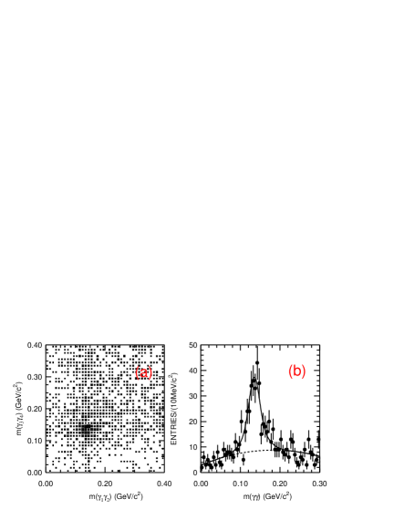
Figure 2: (a) Scatter plot of $\gamma_{1}\gamma_{2}$ versus $\gamma_{3}\gamma_{4}$ invariant mass for $\psi(2S)\rightarrow\pi^{0}\pi^{0}p\overline{p}$ candidate events. (b) Invariant mass distribution of $\gamma_{1}\gamma_{2}$ after requiring $|m_{\gamma_{3}\gamma_{4}}-m_{\pi^{o}}|<0.03~{}\mbox{GeV}/c^{2}$. The data are fitted with a double Gaussian function and a second order background polynomial.

For $\psi(2S)\rightarrow\gamma\pi^{0}p\overline{p}$, candidate events must have two charged tracks and three good photons. To reject background from $\psi(2S)\rightarrow\pi^{0}\pi^{0}J/\psi,J/\psi\rightarrow p\overline{p}$ events, the $p\overline{p}$ invariant mass is required to satisfy $|m_{p\overline{p}}-m_{J/\psi}|>0.1~{}\mbox{GeV}/c^{2}$.

Figure 3 (a) shows the $\gamma\gamma$ invariant mass distribution for $\psi(2S)\rightarrow\gamma\gamma\gamma p\overline{p}$ candidate events, where $\gamma\gamma$ is any possible combination among the three photon candidates. There is a clear $\pi^{0}$ signal. The distribution is fitted with a double Gaussian function with parameters determined from MC simulation plus a second order polynomial for the background. The number of events determined from the fit is $345\pm 33$.

Background studies indicate that the main contamination to the $\pi^{0}$ signal comes from $\psi(2S)\rightarrow\pi^{0}\pi^{0}p\overline{p}$ and $\pi^{0}p\overline{p}$; other backgrounds only contribute a smooth background. All possible backgrounds, including continuum, known simulated backgrounds ($\psi(2S)\rightarrow\pi^{0}\pi^{0}p\overline{p}$ and $\pi^{0}p\overline{p}$), and other unknown backgrounds estimated from the $\psi(2S)$ inclusive MC sample, are combined in Fig. 3 (b). Fitting this distribution in the same way as in Fig. 3 (a), the number of peaking background events is estimated to be $219\pm 18$.

Just as for $\psi(2S)\rightarrow\pi^{0}\pi^{0}p\overline{p}$, no significant intermediate process is observed in $\psi(2S)\rightarrow\gamma\pi^{0}p\overline{p}$. The efficiency is determined to be 8.94% with a phase space generator, and the branching fraction is calculated to be

$${\cal B}(\psi(2S)\rightarrow\gamma\pi^{0}p\overline{p})=(1.0\pm 0.3)\times 10^{-4},$$

where the error is statistical.

Figure 3: Distributions of $\gamma\gamma$ invariant mass for $\psi(2S)\rightarrow\gamma\gamma\gamma p\overline{p}$ candidate events fitted with a double Gaussian function and a second order background polynomial. (a) signal and (b) backgrounds including continuum, known simulated backgrounds ($\psi(2S)\rightarrow\pi^{0}\pi^{0}p\overline{p}$ and $\pi^{0}p\overline{p}$), and other unknown backgrounds estimated from the $\psi(2S)$ inclusive MC sample.

For $\psi(2S)\rightarrow\pi^{0}p\overline{p}$, there is an earlier measurement from BESII ppbpi0-bes2 . We reanalyze this channel in the same way, and then extract the $m_{p\overline{p}}$ distribution and estimate its contamination to $\psi(2S)\rightarrow\gamma p\overline{p}$.

Candidate events are required to have two charged tracks and two good photons. The probability of the 4C-fit must be greater than 1%, and the probability of the 4C-fit for the $\psi(2S)\rightarrow\gamma\gamma p\overline{p}$ hypothesis must be greater than that for $\psi(2S)\rightarrow\gamma\gamma K^{+}K^{-}$. To reject background from $\psi(2S)\rightarrow\pi^{0}\pi^{0}J/\psi,J/\psi\rightarrow p\overline{p}$ events, the invariant mass of $p\overline{p}$ is required to be: $|m_{p\overline{p}}-m_{J/\psi}|>0.02~{}\mbox{GeV}/c^{2}$.

A fit to the $m_{\gamma\gamma}$ distribution is performed with a double Gaussian function with parameters determined from MC simulation plus a second order polynomial for the background for $\psi(2S)\rightarrow\gamma\gamma p\overline{p}$ candidate events. The number of events determined from the fit is $266\pm 20$, and the detection efficiency is 14.8%. The branching fraction is determined to be:

$${\cal B}(\psi(2S)\rightarrow\pi^{0}p\overline{p})=(13.0\pm 1.0)\times 10^{-6},$$

where the error is statistical. This measurement agrees well with the previous BESII result of ($13.2\pm 1.0\pm 1.5)\times 10^{-6}$ ppbpi0-bes2 .

V.1.2 Signal Analysis

For $\psi(2S)\rightarrow\gamma p\overline{p}$, 329 events are observed after the event selection described in Section III; the $p\overline{p}$ invariant mass distribution is shown in Fig. 4. After subtracting the normalized major backgrounds, $\psi(2S)\to\pi^{0}\pi^{0}p\bar{p}$, $\gamma\pi^{0}p\bar{p}$, and $\pi^{0}p\bar{p}$, the number of signal events is $142\pm 18$. The detection efficiency determined from MC simulation is 35.3%, and the branching fraction for this process is determined to be:

$${\cal B}(\psi(2S)\rightarrow\gamma p\overline{p})=(2.9\pm 0.4)\times 10^{-5},$$

where the error is statistical.

There is an excess of events between $p\overline{p}$ threshold and $2.5~{}\mbox{GeV}/c^{2}$, but no significant narrow structure due to the $X(1859)$, that was observed in $J/\psi\rightarrow\gamma p\overline{p}$ jpsi-gppb . A fit to the mass spectrum (see Fig. 5) with an acceptance-weighted $S$-wave Breit-Wigner for the $X$ resonance (with mass and width fixed to $1859~{}\mbox{MeV}/c^{2}$ and $30~{}\mbox{MeV}/c^{2}$, respectively), together with the normalized MC histograms for the above measured background channels ($\psi(2S)\to\pi^{0}\pi^{0}p\bar{p}$, $\gamma\pi^{0}p\bar{p}$, and $\pi^{0}p\bar{p}$) and the histogram from $\psi(2S)\to\gamma p\bar{p}$ phase space massres , yields $11.7\pm 6.7$ events with a statistical significance of 2.0 $\sigma$. The upper limit on the branching fraction is determined to be

$${\cal B}(\psi(2S)\rightarrow\gamma X(1859)\rightarrow\gamma p\overline{p})<5.4\times 10^{-6}$$

at the 90% C.L.

Figure 4: The $p\overline{p}$ invariant mass distribution for $\psi(2S)\rightarrow\gamma p\overline{p}$ candidate events (dots with error bars). The shaded histogram is the sum of all backgrounds, including continuum, known simulated backgrounds ($\psi(2S)\to\pi^{0}\pi^{0}p\bar{p}$, $\gamma\pi^{0}p\bar{p}$, and $\pi^{0}p\bar{p}$), and other unknown backgrounds estimated from the $\psi(2S)$ inclusive MC sample.

Figure 5: The fit to the $m_{p\overline{p}}-2m_{p}$ distribution of $\psi(2S)\rightarrow\gamma p\overline{p}$ candidate events. The solid histogram is the fit result, the lower dashed line is the $X$ resonance shape, the dash-dotted histogram is the shape for $\psi(2S)\to\gamma p\bar{p}$ phase-space, the dotted histogram is the measured background channels ($\psi(2S)\to\pi^{0}\pi^{0}p\bar{p}$, $\gamma\pi^{0}p\bar{p}$, and $\pi^{0}p\bar{p}$), and the top dashed line is the efficiency curve.

V.2 $\psi(2S)\rightarrow\gamma 2(\pi^{+}\pi^{-})$

For $\psi(2S)\rightarrow\gamma 2(\pi^{+}\pi^{-})$, the main background comes from $\psi(2S)\rightarrow 2(\pi^{+}\pi^{-})\pi^{0}$, so we first measure $\psi(2S)\rightarrow 2(\pi^{+}\pi^{-})\pi^{0}$ in order to be able to estimate its contamination to $\psi(2S)\rightarrow\gamma 2(\pi^{+}\pi^{-})$.

V.2.1 Background analysis

For $\psi(2S)\rightarrow\pi^{0}2(\pi^{+}\pi^{-})$, candidate events are required to have four charged tracks and two good photons. The probability of the 4C-fit must be greater than 1%, the $\chi^{2}_{comb}$ probability for the $\psi(2S)\rightarrow\pi^{0}2(\pi^{+}\pi^{-})$ hypothesis must be greater than those of $\psi(2S)\rightarrow\pi^{0}K^{+}K^{-}\pi^{+}\pi^{-}$ and $\psi(2S)\rightarrow\pi^{0}\pi^{+}\pi^{-}p\overline{p}$, and the sum of the momentum of any $\pi^{+}$ and $\pi^{-}$ pairs must be greater than $550~{}\mbox{MeV}/c$ to reject contamination from $\psi(2S)\rightarrow\pi^{+}\pi^{-}J/\psi$ events.

After the above selection, a clear $\pi^{0}$ signal can be seen in the $\gamma\gamma$ invariant mass distribution of $\psi(2S)\rightarrow 2(\pi^{+}\pi^{-})\gamma\gamma$ candidates. After subtracting backgrounds, such as $\psi(2S)\to\gamma\chi_{c0},\chi_{c0}\to 2(\pi^{+}\pi^{-})$, $\psi(2S)\to\pi^{0}\pi^{0}J/\psi,J/\psi\to 2(\pi^{+}\pi^{-})$, etc., in the $\gamma\gamma$ invariant mass spectrum, the distribution is fitted with a $\pi^{0}$ signal shape determined with MC simulation plus a second order polynomial for the other remaining backgrounds, and the number of $\pi^{0}$ signal events is $2173\pm 53$. The detection efficiency is determined to be 6.32% taking into consideration the significant intermediate states such as $\omega\pi^{+}\pi^{-}$, $\omega f_{2}(1270)$, and $b_{1}^{\pm}\pi^{\mp}$ described below.

Figure 6 (b) shows the $\pi^{+}\pi^{-}\pi^{0}$ invariant mass distribution for events satisfying $|m_{\gamma\gamma}-m_{\pi^{o}}|<0.03~{}\mbox{GeV}/c^{2}$. The fit is performed with an $\omega$ signal shape plus a second order polynomial for the background, and the number of $\omega$ signal events obtained is $386\pm 23$. The efficiency determined from MC simulation is 3.74% correcting for intermediate states, such as $\omega f_{2}(1270)$ and $b_{1}^{\pm}\pi^{\mp}$, described below.

Figure 6 (c) shows the distribution of $\pi^{+}\pi^{-}$ invariant mass recoiling against the $\omega$, selected with the requirements $|m_{\pi^{+}\pi^{-}\pi^{0}}-m_{\omega}|<0.05~{}\mbox{GeV}/c^{2}$ and $|m_{\omega\pi}-m_{b_{1}}|>0.2~{}\mbox{GeV}/c^{2}$ to reject $b_{1}^{\pm}\pi^{\mp}$ events. The invariant mass spectrum is fitted with a $\sigma$, a $f_{2}(1270)$ shape determined from MC simulation, and a second order polynomial to describe other backgrounds. The number of $f_{2}(1270)$ events obtained is $57\pm 13$, and the detection efficiency determined from MC simulation is 3.65%.

Figure 6 (d) shows the $\omega\pi^{\pm}$ invariant mass spectrum with the requirement $|m_{\pi^{+}\pi^{-}\pi^{0}}-m_{\omega}|<0.05~{}\mbox{GeV}/c^{2}$. A clear $b_{1}^{\pm}$ signal is seen. Fitting with a $b_{1}$ signal shape with the mass and width fixed to PDG values plus a background polynomial, the number of $b_{1}^{\pm}$ signal events is $202\pm 21$, and the detection efficiency determined from MC simulation is 3.24%. The branching fractions of these processes are determined to be:

$${\cal B}(\psi(2S)\rightarrow\pi^{0}2(\pi^{+}\pi^{-}))=(24.9\pm 0.7)\times 10^{-4},$$

$${\cal B}(\psi(2S)\rightarrow\omega\pi^{+}\pi^{-})=(8.4\pm 0.5)\times 10^{-4},$$

$${\cal B}(\psi(2S)\rightarrow\omega f_{2}(1270))=(2.3\pm 0.5)\times 10^{-4},$$

$${\cal B}(\psi(2S)\rightarrow b_{1}^{\pm}\pi^{\mp})=(5.1\pm 0.6)\times 10^{-4},$$

where the errors are statistical.

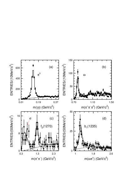
Figure 6: Invariant mass distributions with fits for $\psi(2S)\rightarrow\pi^{0}2(\pi^{+}\pi^{-})$ candidates, where dots with error bars are data, and the solid histograms and curves are the fit results. (a) $\gamma\gamma$; (b) $\pi^{+}\pi^{-}\pi^{0}$ with $|m_{\gamma\gamma}-m_{\pi^{o}}|<0.03~{}\mbox{GeV}/c^{2}$; (c) $\pi^{+}\pi^{-}$ with $|m_{\pi^{+}\pi^{-}\pi^{0}}-m_{\omega}|<0.05~{}\mbox{GeV}/c^{2}$ and $b_{1}^{\pm}\pi^{\mp}$ events rejected; and (d) $\omega\pi^{\pm}$ for the $\psi(2S)\rightarrow\pi^{0}2(\pi^{+}\pi^{-})$ candidate events. Resonance parameters are fixed to their world averaged values PDG .

V.2.2 Signal analysis

For $\psi(2S)\rightarrow\gamma 2(\pi^{+}\pi^{-})$, candidate events require four charged tracks, and each track must be identified as a pion. The background from $\psi(2S)\rightarrow\pi^{+}\pi^{-}J/\psi$ is rejected by requiring $|m_{recoil}^{\pi^{+}\pi^{-}}-m_{J/\psi}|>0.05$ GeV/$c^{2}$. After selection, 1697 candidates remain, and the $2(\pi^{+}\pi^{-})$ invariant mass distribution for the candidate events is shown in Fig. 7. The backgrounds include contributions from the continuum (estimated from the data sample at $\sqrt{s}=3.65~{}\mbox{GeV}$), $\psi(2S)\rightarrow\pi^{0}2(\pi^{+}\pi^{-})$, backgrounds remaining from $\pi^{+}\pi^{-}J/\psi,J/\psi\rightarrow\rho\pi$ and $\pi^{0}K^{0}_{S}K^{+}\pi^{-}+c.c.$, and the other unknown backgrounds assuming that they have the same shape as that obtained from the inclusive $\psi(2S)$ MC sample.

Using the $\chi^{2}$ fitting method of Section IV, the number of signal events is $583\pm 41$. The detection efficiency determined from MC simulation is 10.4%, and the branching fraction for this process is determined to be:

$${\cal B}(\psi(2S)\rightarrow\gamma 2\pi^{+}\pi^{-})=(39.6\pm 2.8)\times 10^{-5},$$

where the error is statistical.

Figure 7: The $2(\pi^{+}\pi^{-})$ invariant mass distribution for $\psi(2S)\rightarrow\gamma 2(\pi^{+}\pi^{-})$ candidate events (dots with error bars). The shaded histogram includes contributions from the continuum (estimated from the data sample at $\sqrt{s}=3.65~{}\mbox{GeV}$), $\psi(2S)\rightarrow\pi^{0}2(\pi^{+}\pi^{-})$, backgrounds remaining from $\pi^{+}\pi^{-}J/\psi,J/\psi\rightarrow\rho\pi$ and $\pi^{0}K^{0}_{S}K^{+}\pi^{-}+c.c.$, and other unknown backgrounds estimated from the inclusive $\psi(2S)$ MC sample.

V.3 $\psi(2S)\rightarrow\gamma K^{0}_{S}K^{+}\pi^{-}+c.c.$

For $\psi(2S)\rightarrow\gamma K^{0}_{S}K^{\pm}\pi^{\mp}$, the main background comes from $\psi(2S)\rightarrow K^{0}_{S}K^{\pm}\pi^{\mp}\pi^{0}$, so we first measure $\psi(2S)\rightarrow K^{0}_{S}K^{\pm}\pi^{\mp}\pi^{0}$ in order to estimate its contamination to $\psi(2S)\rightarrow\gamma K^{0}_{S}K^{\pm}\pi^{\mp}$.

V.3.1 Background estimation

For $\psi(2S)\rightarrow\pi^{0}K^{0}_{S}K^{+}\pi^{-}+c.c.$, candidate events require four charged tracks and two good photons. Figure 8 shows the scatter plot of $\pi^{+}\pi^{-}$ invariant mass versus the decay length in the transverse plane ($L_{xy}$) of $K^{0}_{S}$ candidates, where a clear $K^{0}_{S}$ signal is observed. Candidate events are required to have only one $K^{0}_{S}$ candidate satisfying the requirements $|m_{\pi^{+}\pi^{-}}-m_{K_{S}^{0}}|<0.015~{}\mbox{GeV}/c^{2}$ and $L_{xy}>0.5$ cm. After $K^{0}_{S}$ selection, the remaining two tracks are identified using their $\chi^{2}_{K\pi}$ values, i.e., if $\chi^{2}_{K^{+}\pi^{-}}<\chi^{2}_{\pi^{+}K^{-}}$, the final state is considered to be $\gamma\gamma K^{0}_{S}K^{+}\pi^{-}$; if $\chi^{2}_{K^{-}\pi^{+}}<\chi^{2}_{\pi^{-}K^{+}}$, the final state is considered to be $\gamma K^{0}_{S}K^{-}\pi^{+}$, where $\chi^{2}_{K\pi}=\chi^{2}_{PID}(K)+\chi^{2}_{PID}(\pi)$.

The confidence level of the 4C-fit must be greater than 1%, and the sum of the momentum of any $\pi^{+}$ and $\pi^{-}$ pair greater than $550~{}\mbox{MeV}/c$ to reject contamination from $\psi(2S)\rightarrow\pi^{+}\pi^{-}J/\psi$ events.

Figure 8: The scatter plot of $\pi^{+}\pi^{-}$ invariant mass versus the $K^{0}_{S}$ decay length for $\psi(2S)\rightarrow\gamma\gamma K^{0}_{S}K^{+}\pi^{-}+c.c.$ candidate events.

After requiring $|m_{\pi^{+}\pi^{-}}-m_{K_{S}^{0}}|<0.015~{}\mbox{GeV}/c^{2}$, the $\gamma\gamma$ invariant mass is shown in Fig. 9 (a), and a clear $\pi^{0}$ signal is seen. After requiring $|m_{\gamma\gamma}-m_{\pi^{o}}|<0.03~{}\mbox{GeV}/c^{2}$, the $\pi^{\pm}\pi^{0}$ invariant mass is shown in Fig. 9 (b), where there is a clear $\rho^{\pm}$ signal.

Figure 9: Invariant mass spectra of (a) $\gamma\gamma$ and (b) $\pi^{\pm}\pi^{0}$ for $\psi(2S)\rightarrow\gamma\gamma K^{0}_{S}K^{\pm}\pi^{\mp}$ candidate events. Dots with error bars are data, the histograms are the fits using signal shapes determined from Monte Carlo simulation and second order polynomials for background, and the dashed curves are the background shapes from the fit.

The $\gamma\gamma$ invariant mass distribution is fitted with a $\pi^{0}$ signal shape determined with MC simulation plus a second order polynomial for the background, and the result is shown in Fig. 9 (a). The number of $\pi^{0}$ signal events fitted is $361\pm 25$, and the efficiency determined from MC simulation is 4.40%, including the effect of the intermediate $K^{\pm}\rho^{\mp}K^{0}_{S}$ state.

The $\pi^{\pm}\pi^{0}$ invariant mass distribution is fitted with a $\rho^{\pm}$ signal shape determined with MC simulation plus a second order polynomial for the background, and the fit result is shown in Fig. 9 (b). The number of $\rho^{\pm}$ signal events is $100\pm 20$, and the detection efficiency is 3.80% determined from MC simulation. The branching fractions of these two processes are determined to be

$${\cal B}(\psi(2S)\rightarrow\pi^{0}K^{0}_{S}K^{\pm}\pi^{\mp})=(8.9\pm 0.6)\times 10^{-4},$$

$${\cal B}(\psi(2S)\rightarrow K^{\pm}\rho^{\mp}K^{0}_{S})=(2.9\pm 0.6)\times 10^{-4},$$

where the errors are statistical.

V.3.2 Signal analysis

The event selection is similar to $\psi(2S)\rightarrow\pi^{0}K^{0}_{S}K^{+}\pi^{-}+c.c.$, but only one photon is required. After event selection, the $\pi^{+}\pi^{-}$ invariant mass distribution is shown in Fig. 10. A fit is performed with a histogram describing the $K^{0}_{S}$ shape obtained from MC simulation, the normalized histogram for $\psi(2S)\rightarrow\pi^{0}K^{0}_{S}K^{+}\pi^{-}+c.c.$ background, and a Legendre polynomial for the other smooth backgrounds. The fit yields $115\pm 16$ events. The detection efficiency is 4.83%, and the branching fraction is determined to be:

$${\cal B}(\psi(2S)\rightarrow\gamma K^{0}_{S}K^{+}\pi^{-}+c.c.)=(25.6\pm 3.6)\times 10^{-5},$$

where the error is statistical. Figure 11 shows the $K^{0}_{S}K^{\pm}\pi^{\mp}$ invariant mass distribution after event selection.

Figure 10: The $\pi^{+}\pi^{-}$ invariant mass distribution for $\psi(2S)\rightarrow\gamma K^{0}_{S}K^{+}\pi^{-}+c.c.$ candidate events. Dots with error bars are data. The histogram is the fit with a histogram describing the $K^{0}_{S}$ shape obtained from MC simulation, the normalized histogram for $\psi(2S)\rightarrow\pi^{0}K^{0}_{S}K^{+}\pi^{-}+c.c.$ background (dashed histogram), and a Legendre polynomial for the other smooth backgrounds (dotted histogram).

Figure 11: The $K^{0}_{S}K^{\pm}\pi^{\mp}$ invariant mass distribution for $\psi(2S)\rightarrow\gamma K^{0}_{S}K^{+}\pi^{-}+c.c.$ candidates (dots with error bars). The shaded histogram is the sum of backgrounds including $\psi(2S)\rightarrow\pi^{0}K^{0}_{S}K^{+}\pi^{-}+c.c.$ and continuum background.

V.4 $\psi(2S)\rightarrow\gamma K^{+}K^{-}\pi^{+}\pi^{-}$

For $\psi(2S)\rightarrow\gamma K^{+}K^{-}\pi^{+}\pi^{-}$, candidate events require four charged tracks, among which two tracks must be identified as pions and the other two tracks identified as kaons. The background from $\psi(2S)\rightarrow\pi^{+}\pi^{-}J/\psi$ is rejected by requiring $|m_{recoil}^{\pi^{+}\pi^{-}}-m_{J/\psi}|>0.05$ GeV/$c^{2}$, the background from $\psi(2S)\to\gamma 2(\pi^{+}\pi^{-})$ is rejected by requiring $\chi^{2}_{\gamma K^{+}K^{-}\pi^{+}\pi^{-}}<\chi^{2}_{\gamma 2(\pi^{+}\pi^{-})}$, and the background from $\psi(2S)\to\gamma K^{0}_{S}K^{+}\pi^{-}+c.c.$ is rejected by requiring $|m_{\pi^{+}\pi^{-}}-m_{K_{S}^{0}}|>0.04$ GeV/$c^{2}$.

Figure 12 shows the $K^{+}K^{-}\pi^{+}\pi^{-}$ invariant mass distribution after event selection, where 361 events are observed. The backgrounds mainly come from $\psi(2S)\rightarrow\pi^{0}K^{+}K^{-}\pi^{+}\pi^{-}$ final states including intermediate states.

Using the $\chi^{2}$ fitting method of Section IV, the number of signal events is $132\pm 19$. The detection efficiency determined from MC simulation is 4.94%, and the branching fraction for this process is determined to be:

$${\cal B}(\psi(2S)\rightarrow\gamma K^{+}K^{-}\pi^{+}\pi^{-})=(19.1\pm 2.7)\times 10^{-5},$$

where the error is statistical.

Figure 12: The $K^{+}K^{-}\pi^{+}\pi^{-}$ invariant mass distribution for $\psi(2S)\rightarrow\gamma K^{+}K^{-}\pi^{+}\pi^{-}$ candidates (dots with error bars). The shaded histogram is background which mainly comes from $\psi(2S)\rightarrow\pi^{0}K^{+}K^{-}\pi^{+}\pi^{-}$.

V.5 $\psi(2S)\rightarrow\gamma K^{\ast 0}K^{+}\pi^{-}+c.c.$ and $\psi(2S)\rightarrow\gamma K^{\ast 0}\bar{K^{\ast 0}}+c.c.$

We apply the same event selection criteria as for $\psi(2S)\rightarrow\gamma K^{+}K^{-}\pi^{+}\pi^{-}$. For this decay channel, the main background channels are from $\psi(2S)\rightarrow K^{\ast 0}K^{-}\pi^{+}\pi^{0}+c.c.$ (phase space), $\psi(2S)\rightarrow K^{\ast 0}K^{-}\rho^{+}+c.c.$, and $\psi(2S)\rightarrow K^{\ast 0}\overline{K}^{\ast 0}\pi^{0}$.

Using a Breit-Wigner function to describe the signal along with the sum of normalized histograms from the $\psi(2S)\rightarrow K^{\ast 0}K^{-}\pi^{+}\pi^{0}+c.c.$ (phase space), $\psi(2S)\rightarrow K^{\ast 0}K^{-}\rho^{+}+c.c.$, and $\psi(2S)\rightarrow K^{\ast 0}\overline{K}^{\ast 0}\pi^{0}$ background channels, and a second order Legendre polynomial to describe other remaining backgrounds to fit the $K^{\pm}\pi^{\mp}$ invariant mass spectrum, $237\pm 39$ $\psi(2S)\rightarrow\gamma K^{\ast 0}K^{-}\pi^{+}+c.c.$ candidate events are obtained, as shown in Fig. 13. Events from the intermediate state $\psi(2S)\rightarrow\gamma K^{\ast 0}\overline{K}^{\ast 0}$ are counted twice, so an efficiency correction must be made for this.

Figure 13: The $K^{\pm}\pi^{\mp}$ invariant mass distribution for $\psi(2S)\rightarrow\gamma K^{+}K^{-}\pi^{+}\pi^{-}$ candidates. Dots with error bars are data. The blank histogram is the result of a fit using a Breit-Wigner function to describe the signal along with the sum of normalized histograms from the $\psi(2S)\rightarrow K^{\ast 0}K^{-}\pi^{+}\pi^{0}+c.c.$ (phase space), $\psi(2S)\rightarrow K^{\ast 0}K^{-}\rho^{+}+c.c.$, and $\psi(2S)\rightarrow K^{\ast 0}\overline{K}^{\ast 0}\pi^{0}$ background channels, and a second order Legendre polynomial to describe other remaining backgrounds. The dashed histogram is the fitted sum of all backgrounds.

The scatter plot of $K^{+}\pi^{-}$ versus $K^{-}\pi^{+}$ invariant mass is shown in Fig. 14, where clear $K^{\ast 0}$ and $\overline{K}^{\ast 0}$ signals are seen. The numbers of $\psi(2S)\rightarrow\gamma K^{\ast 0}\overline{K}^{\ast 0}$ events and background events are estimated from the scatter plot. The signal region is shown as a square box at (0.896, 0.896)$~{}\mbox{GeV}/c^{2}$ with a width of $60~{}\mbox{MeV}/c^{2}$. Backgrounds are estimated from sideband boxes, which are taken 60 MeV$/c^{2}$ away from the signal box. Background in the horizontal or vertical sideband boxes is twice that in the signal region. If we subtract half the number of events in the horizontal and vertical sideband boxes, we double count the phase space background. Therefore the background is one-half the number of events in the horizontal and vertical boxes plus one fourth the number of the events in the four corner boxes. After subtraction, $41\pm 8$ $\psi(2S)\rightarrow\gamma K^{\ast 0}\overline{K}^{\ast 0}$ candidates are obtained, and the efficiency is $(2.75\pm 0.06)\%$. In simulating signal channels containing $K^{\ast}$, the shape of $K^{\ast}$ is described by a P-wave relativistic Breit-Wigner, with a width

$$\Gamma=\Gamma_{0}\frac{m_{0}}{m}\frac{1+r^{2}p_{0}^{2}}{1+r^{2}p^{2}}\Big{[}\frac{p}{p_{0}}\Big{]}^{3},$$

where $m$ is the mass of the $K\pi$ system, $p$ is the momentum of the kaon in the $K\pi$ system, $\Gamma_{0}$ is the width of the resonance, $m_{0}$ is the mass of the resonance, $p_{0}$ is the momentum evaluated at the resonance mass, $r$ is the interaction radius, and $\frac{1+r^{2}p_{0}^{2}}{1+r^{2}p^{2}}$ represents the contribution of the barrier factor. The value $r=(3.4\pm 0.6\pm 0.3)(~{}\mbox{GeV}/c)^{-1}$ measured by the $K^{-}\pi^{+}$ scattering experiment r-aston is used as an approximate estimation of the interaction radius $r$.

Figure 14: The scatter plot of $K^{+}\pi^{-}$ versus $K^{-}\pi^{+}$ invariant mass of $\psi(2S)\rightarrow\gamma K^{+}K^{-}\pi^{+}\pi^{-}$ candidate events. The center box indicates the signal region for $\psi(2S)\rightarrow\gamma K^{\ast 0}\overline{K}^{\ast 0}$ events, and the other boxes are used for background determination.

Taking into consideration the effect of the intermediate channel, $\psi(2S)\to\gamma K^{*0}\bar{K^{*0}}$, the efficiency for $\psi(2S)\rightarrow\gamma K^{\ast}K^{-}\pi^{+}+c.c.$ is 6.86%, and we obtain the branching fractions:

$${\cal B}(\psi(2S)\rightarrow\gamma K^{\ast}K^{-}\pi^{+}+c.c.)=(37.0\pm 6.1)\times 10^{-5}$$

$${\cal B}(\psi(2S)\rightarrow\gamma K^{\ast 0}\overline{K}^{\ast 0})=(24.0\pm 4.5)\times 10^{-5},$$

where the errors are statistical.

V.6 $\psi(2S)\rightarrow\gamma 2(K^{+}K^{-})$

For $\psi(2S)\rightarrow\gamma 2(K^{+}K^{-})$, the candidate events must have four charged tracks, and every track must be identified as a kaon. The backgrounds from $\psi(2S)\rightarrow\gamma 2(\pi^{+}\pi^{-}),\gamma\pi^{+}\pi^{-}K^{+}K^{-}$ are rejected by requiring the $\chi^{2}_{4C}$ for the signal channel to be less than those for backgrounds. There are 15 events observed after event selection, and the $2(K^{+}K^{-})$ invariant mass distribution is shown in Fig. 15. The detection efficiency for this channel is 2.93%.

Figure 15: Invariant mass distribution of $2(K^{+}K^{-})$ for $\psi(2S)\rightarrow\gamma 2(K^{+}K^{-})$ candidates (dots with error bars). The shaded histograms is background mainly from $\psi(2S)\to\pi^{0}2(K^{+}K^{-})$.

The dominant background comes from $\psi(2S)\rightarrow\pi^{0}2(K^{+}K^{-})$. Using the branching fraction measured by CLEO chic23hs , the estimated number of background events remaining is $8\pm 2$. To measure the continuum contribution in this channel, the continuum data at $E_{cm}=3.65~{}\mbox{GeV}$ is analyzed using the same criteria as for $\psi(2S)$ data, and no events survive. It is also found that no events survive from the simulated 14 million inclusive $\psi(2S)$ decay MC sample. The upper limit on the number of $\psi(2S)\rightarrow\gamma 2(K^{+}K^{-})$ events is 14 at the 90% C.L., and the corresponding upper limit on the branching fraction after considering systematic uncertainties is

$${\cal B}(\psi(2S)\rightarrow\gamma 2(K^{+}K^{-}))<4.0\times 10^{-5}.$$

V.7 $\psi(2S)\rightarrow\gamma\pi^{+}\pi^{-}p\overline{p}$

For $\psi(2S)\rightarrow\gamma\pi^{+}\pi^{-}p\overline{p}$, there must be four good charged tracks, and two of them must be identified as a proton anti-proton pair. The backgrounds from $\gamma 2(\pi^{+}\pi^{-})$ and $\gamma\pi^{+}\pi^{-}K^{+}K^{-}$ are rejected by requiring $\chi^{2}_{4C}$ for the signal channel to be less than for the background channels. To eliminate possible contamination from $\psi(2S)\rightarrow\pi^{+}\pi^{-}J/\psi,J/\psi\to\gamma p\overline{p}$, we require $|m^{\pi^{+}\pi^{-}}_{recoil}-m_{J/\psi}|>0.02~{}\mbox{GeV}/c^{2}$.

Figure 16 shows the $\pi^{+}\pi^{-}p\overline{p}$ invariant mass distribution with 55 events after event selection. The detection efficiency for this channel is 4.47%.

Figure 16: Invariant mass distribution of $\pi^{+}\pi^{-}p\overline{p}$ for $\psi(2S)\rightarrow\gamma\pi^{+}\pi^{-}p\overline{p}$ candidates (dots with error bars). The shaded histogram is background mainly from $\psi(2S)\rightarrow\pi^{0}\pi^{+}\pi^{-}p\overline{p}$ and $\psi(2S)\rightarrow\pi^{+}\pi^{-}J/\psi,J/\psi\rightarrow\gamma p\overline{p}$.

The dominant backgrounds are $\psi(2S)\rightarrow\pi^{0}\pi^{+}\pi^{-}p\overline{p}$ and background remaining from $\psi(2S)\rightarrow\pi^{+}\pi^{-}J/\psi,J/\psi\rightarrow\gamma p\overline{p}$. The detection efficiencies for these two background channels are determined by MC simulation to be 0.35% and 0.18%, respectively. For the first background channel, using ${\cal B}(\psi(2S)\rightarrow\pi^{0}\pi^{+}\pi^{-}p\overline{p})$ measured by CLEO chic23hs , the number of background events remaining is estimated to be $35.8\pm 3.5$. Similarly, the estimated number of background events from $\psi(2S)\rightarrow\pi^{+}\pi^{-}J/\psi,J/\psi\rightarrow\gamma p\overline{p}$ is $1.7\pm 0.4$. Subtracting backgrounds, the number of $\psi(2S)\rightarrow\gamma\pi^{+}\pi^{-}p\overline{p}$ events is $17\pm 7$, and the corresponding branching fraction is

$${\cal B}(\psi(2S)\rightarrow\gamma\pi^{+}\pi^{-}p\overline{p})=(2.8\pm 1.2)\times 10^{-5},$$

where the error is statistical.

V.8 $\psi(2S)\rightarrow\gamma 3(\pi^{+}\pi^{-})$

For $\psi(2S)\rightarrow\gamma 3(\pi^{+}\pi^{-})$, six charged tracks are required. The backgrounds from $\psi(2S)\rightarrow\pi^{+}\pi^{-}J/\psi$ and $\psi(2S)\rightarrow K^{0}_{S}K^{0}_{S}\pi^{+}\pi^{-}$ are removed by eliminating events having the recoil mass of any pion pair satisfying $|m^{\pi^{+}\pi^{-}}_{recoil}-m_{J/\psi}|<0.05~{}\mbox{GeV}/c^{2}$ or having a pion pair in the $K_{S}^{0}$ mass region from 0.47 to 0.53 GeV/$c^{2}$. The remaining backgrounds mainly come from processes with multi-photon final states, such as $\psi(2S)\rightarrow\pi^{0}3(\pi^{+}\pi^{-}),\gamma\pi^{0}3(\pi^{+}\pi^{-}),$ and $\pi^{0}\pi^{0}3(\pi^{+}\pi^{-})$. Their contaminations are estimated using MC simulation. Figure 17 shows the $3(\pi^{+}\pi^{-})$ invariant mass distribution after event selection with 118 events observed. The detection efficiency for this channel is 1.97%. Using the $\chi^{2}$ fitting method described in Section IV, the upper limit on the number of signal events is 45 at the 90 % C.L., and the upper limit on the branching fraction after considering systematic uncertainties is $B(\psi(2S)\to\gamma 3(\pi^{+}\pi^{-}))<17\times 10^{-5}$.

Figure 17: The $3(\pi^{+}\pi^{-})$ invariant mass distribution for $\psi(2S)\rightarrow\gamma 3(\pi^{+}\pi^{-})$ candidates (dots with error bars). The shaded histogram is background mainly from processes with multi-photon final states, such as $\psi(2S)\rightarrow\pi^{0}3(\pi^{+}\pi^{-}),\gamma\pi^{0}3(\pi^{+}\pi^{-}),$ and $\pi^{0}\pi^{0}3(\pi^{+}\pi^{-})$.

V.9 $\psi(2S)\rightarrow\gamma 2(\pi^{+}\pi^{-})K^{+}K^{-}$

V.9.1 Background estimation

First, background from $\psi(2S)\rightarrow\eta J/\psi$, $\eta\to\gamma\pi^{+}\pi^{-}$, $J/\psi\rightarrow\pi^{+}\pi^{-}K^{+}K^{-}$ is rejected by requiring $m_{2(\pi^{+}\pi^{-})K^{+}K^{-}}<2.9$ GeV$/c^{2}$. The dominant backgrounds remaining are $\psi(2S)\rightarrow\pi^{0}2(\pi^{+}\pi^{-})K^{+}K^{-}$ and $\gamma\pi^{0}2(\pi^{+}\pi^{-})K^{+}K^{-}$. Branching fractions for these are not currently available, so they are measured using our $\psi(2S)$ data sample.

For $\psi(2S)\rightarrow\pi^{0}2(\pi^{+}\pi^{-})K^{+}K^{-}$, the number of good photons is required to be $N_{\gamma}=2$ or $3$. A kinematic fit is performed under the $\psi(2S)\to\gamma\gamma 2(\pi^{+}\pi^{-})K^{+}K^{-}$ hypothesis running over all selected photons, and the combination with the smallest $\chi^{2}$ is retained. Background from $\psi(2S)\rightarrow\pi^{+}\pi^{-}J/\psi$, $J/\psi\rightarrow\gamma\gamma 2(\pi^{+}\pi^{-})K^{+}K^{-}$ is rejected by requiring $|m^{\pi^{+}\pi^{-}}_{recoil}-m_{J/\psi}|>0.05$ $\hbox{GeV}/c^{2}$. The possible backgrounds from $\psi(2S)\to\gamma 2(\pi^{+}\pi^{-})K^{+}K^{-}$ and $3\gamma 2(\pi^{+}\pi^{-})K^{+}K^{-}$ are rejected by requiring the $\chi^{2}$ value for the signal to be less than those for the backgrounds. To remove backgrounds from $\psi(2S)\to\gamma\chi_{cJ}$ decays, we require $m_{2(\pi^{+}\pi^{-})K^{+}K^{-}}<3.38$ GeV$/c^{2}$.

Eight main peaking background channels, including $\psi(2S)\rightarrow\eta J/\psi$, $\pi^{0}J/\psi$ and $\gamma\chi_{cJ}$ to decay into the same final states, are simulated and fitted using the same procedure and selection criteria, and $9.8\pm 4.5$ background events are obtained. Using the 14 million inclusive MC sample, $14.7\pm 5.7$ background events are found, which is consistent with the simulation result within the statistical error.

Figure 18 shows the $\gamma\gamma$ invariant mass distribution for $\psi(2S)\rightarrow\pi^{0}2(\pi^{+}\pi^{-})K^{+}K^{-}$ candidate events. A fit is performed with a $\pi^{0}$ signal shape determined from MC simulation plus a third order polynomial for the background, and the number of $\pi^{0}$ signal events is determined to be $57.4\pm 9.8$. After subtracting peaking backgrounds, the number of signal events is $47.6\pm 10.8$.

The detection efficiency determined from MC simulation using a phase space generator is $0.41\%$ below $m_{2(\pi^{+}\pi^{-})K^{+}K^{-}}=3.38\textrm{ GeV}/c^{2}$, and the branching fraction is determined to be:

$${\cal B}(\psi(2S)\rightarrow\pi^{0}2(\pi^{+}\pi^{-})K^{+}K^{-})=(8.39\pm 1.91)\times 10^{-4}$$

with the requirement $m_{2(\pi^{+}\pi^{-})K^{+}K^{-}}<3.38\textrm{ GeV}/c^{2}$, where the error is statistical. The effect of possible intermediate resonances is not considered. Assuming phase space production, the branching fraction extrapolated to the full $m_{2(\pi^{+}\pi^{-})K^{+}K^{-}}$ energy region is determined to be ${\cal B}(\psi(2S)\rightarrow\pi^{0}2(\pi^{+}\pi^{-})K^{+}K^{-})=(11.5\pm 2.6)\times 10^{-4}$.

Figure 18: The $\gamma\gamma$ invariant mass distribution for $\psi(2S)\rightarrow\gamma\gamma 2(\pi^{+}\pi^{-})K^{+}K^{-}$ candidate events. Dots with error bars are data, and the blank histogram is the fit with a $\pi^{0}$ signal shape determined from MC simulation plus a third order polynomial for the background. The curve is the fitted background.

For $\psi(2S)\rightarrow\gamma\pi^{0}2(\pi^{+}\pi^{-})K^{+}K^{-}$, the number of good photons is required to be $N_{\gamma}=3$ or 4. A kinematic fit is performed under the $\psi(2S)\to 3\gamma 2(\pi^{+}\pi^{-})K^{+}K^{-}$ hypothesis running over the selected photons; the combination with the smallest $\chi^{2}$ is retained. Possible backgrounds from $\psi(2S)\rightarrow(n\gamma)2(\pi^{+}\pi^{-})K^{+}K^{-}$ with $n=1$ $2$ and $4$ and from $\psi(2S)\rightarrow 3\gamma 3(\pi^{+}\pi^{-}),~{}3\gamma\pi^{+}\pi^{-}2(K^{+}K^{-})$, and $3\gamma K^{\pm}\pi^{\mp}2(\pi^{+}\pi^{-})$ are rejected by requiring that the $\chi^{2}$ of the signal is less than those of the backgrounds. Background from $\psi(2S)\to\pi^{+}\pi^{-}J/\psi,~{}J/\psi\to 3\gamma\pi^{+}\pi^{-}K^{+}K^{-}$ is rejected by requiring $|m^{\pi^{-}\pi^{+}}_{recoil}-m_{J/\psi}|>0.05$ GeV/$c^{2}$, and backgrounds from $\psi(2S)\rightarrow\pi^{0}J/\psi,~{}\eta J/\psi,~{}\pi^{0}\pi^{0}J/\psi,~{}J/\psi\to 2(\pi^{+}\pi^{-})K^{+}K^{-}$ are rejected with the requirement $|m_{2(\pi^{+}\pi^{-})K^{+}K^{-}}-m_{J/\psi}|>0.05$ GeV/$c^{2}$. We select the $\pi^{0}$ from the $\gamma\gamma$ combinations as the one with $m_{\gamma\gamma}$ invariant mass closest to $m_{\pi^{0}}$. To remove backgrounds from $\psi(2S)\to\gamma\chi_{cJ}$ decays, $m_{\pi^{0}2(\pi^{+}\pi^{-})K^{+}K^{-}}<3.38$ GeV$/c^{2}$ is required.

After event selection, no significant $\pi^{0}$ candidates are observed. A fit with a $\pi^{0}$ shape determined from MC simulation plus a second order Legendre polynomial for background yields $27.1\pm 8.5$ events. Fitting in the same way a histogram of 20 MC simulated background modes, $21.2\pm 10.6$ background events are obtained. The detection efficiency determined from MC simulation is $5.8\times 10^{-4}$. The upper limit on the branching fraction at the $90\%$ C.L., determined using POLE pole and including systematic uncertainties, is

$$B(\psi(2S)\rightarrow\gamma\pi^{0}2(\pi^{+}\pi^{-})K^{+}K^{-})<3.1\times 10^{-3}.$$

V.9.2 Signal analysis

For $\psi(2S)\rightarrow\gamma 2(\pi^{+}\pi^{-})K^{+}K^{-}$, six charged tracks are required, and two of them must be identified as kaons. The background from $\psi(2S)\rightarrow\pi^{+}\pi^{-}J/\psi,J/\psi\to\gamma+$ four charged particles is removed by requiring $|m^{\pi^{+}\pi^{-}}_{recoil}-m_{J/\psi}|>0.05$ GeV$/c^{2}$, and the backgrounds from $\psi(2S)\to\gamma 3(\pi^{+}\pi^{-}),\gamma K^{\pm}\pi^{\mp}2(\pi^{+}\pi^{-})$ and $\gamma 2(K^{+}K^{-})\pi^{+}\pi^{-}$ are rejected by requiring the $\chi^{2}$ values for the signal to be smaller than for the backgrounds. The background from $\psi(2S)\to\eta J/\psi\to\gamma 2(\pi^{+}\pi^{-})K^{+}K^{-}$ is rejected by requiring $m_{2(\pi^{+}\pi^{-})K^{+}K^{-}}<2.9\textrm{GeV}/c^{2}$.

Figure 19 shows the $2(\pi^{+}\pi^{-})K^{+}K^{-}$ invariant mass distribution, where the shaded histogram is background mainly from $\psi(2S)\rightarrow\pi^{0}2(\pi^{+}\pi^{-})K^{+}K^{-}$ and $\gamma\pi^{0}2(\pi^{+}\pi^{-})K^{+}K^{-}$. For the $\psi(2S)\rightarrow\pi^{0}2(\pi^{+}\pi^{-})K^{+}K^{-}$ background channel, the branching fraction of $(8.39\pm 1.91)\times 10^{-4}$ is used since the MC sample is produced with $m_{2(\pi^{+}\pi^{-})K^{+}K^{-}}<3.38$ $\hbox{GeV}/c^{2}$. After subtracting all backgrounds, 17 events are obtained. The detection efficiency for this channel is 0.69%. The upper limit on the number of signal events is 15.5 at the 90% C.L., and the branching fraction after considering systematic uncertainties is $B(\psi(2S)\to\gamma 2(\pi^{+}\pi^{-})K^{+}K^{-})<22\times 10^{-5}$.

Figure 19: The $2(\pi^{+}\pi^{-})K^{+}K^{-}$ invariant mass distribution for $\psi(2S)\rightarrow\gamma 2(\pi^{+}\pi^{-})K^{+}K^{-}$ candidates (dots with error bars). The shaded histogram is background mainly from $\psi(2S)\rightarrow\pi^{0}2(\pi^{+}\pi^{-})K^{+}K^{-}$ and $\gamma\pi^{0}2(\pi^{+}\pi^{-})K^{+}K^{-}$.

Table 1: Summary of systematic errors (%), where WR, $\varepsilon_{\gamma}$, $K^{0}_{S}$ rec., and MC denote the wire resolution, photon efficiency, the error for $K^{0}_{S}$ reconstruction, and MC statistics, respectively. The sixth column gives the uncertainties due to the $\chi^{2}$ fits or the $K^{\ast}$ fit.

Mode	WR	$\varepsilon_{\gamma}$	PID	$K^{0}_{S}$ rec.	fit	Branching Fractions	Background	$N_{\psi(2S)}$	MC	Total
$\gamma p\overline{p}$	6.3	2.0	4.0	—	—	—	9.4	4.0	0.5	12.8
$\gamma p\overline{p}\pi^{0}$	11.6	6.0	4.0	—	—	—	14.3	4.0	3.0	20.4
$\gamma 2(\pi^{+}\pi^{-})$	5.0	2.0	8.0	—	3.0 ($\chi^{2}$ fit)	—	6.4	4.0	1.0	12.7
$\gamma K^{0}_{S}K^{+}\pi^{-}+c.c.$	5.0	2.0	—	3.4	—	—	11.8	4.0	1.0	14.1
$\gamma K^{+}K^{-}\pi^{+}\pi^{-}$	10.7	2.0	8.0	—	3.0 ($\chi^{2}$ fit)	—	17.2	4.0	2.2	22.6
$\gamma K^{\ast 0}K^{+}\pi^{-}+c.c.$	10.7	2.0	8.0	—	8.8 ($K^{\ast}$ fit)	—	10.0	4.0	1.2	19.5
$\gamma K^{\ast 0}\overline{K}^{*0}$	10.7	2.0	8.0	—	—	—	10.0	4.0	1.1	17.4
$\gamma\pi^{+}\pi^{-}p\overline{p}$	10.4	2.0	8.0	—	—	—	20.6	4.0	1.1	24.9
$\gamma 2(K^{+}K^{-})$	11.1	2.0	8.0	—	—	—	14.2	4.0	1.6	20.3
$\gamma 3(\pi^{+}\pi^{-})$	5.0	2.0	—	—	—	—	—	4.0	2.2	7.0
$\gamma 2(\pi^{+}\pi^{-})K^{+}K^{-}$	8.7	2.0	4.0	—	3.0 ($\chi^{2}$ fit)	—	25.0	4.0	3.0	27.5
$\gamma\pi^{0}2(\pi^{+}\pi^{-})K^{+}K^{-}$	9.1	6.0	4.0	—	—	—	6.0	4.0	3.1	14.0
$p\overline{p}\pi^{0}\pi^{0}$	11.7	8.0	4.0	—	—	—	4.3	4.0	1.7	15.9
$\pi^{0}2(\pi^{+}\pi^{-})$	10.0	4.0	8.0	—	—	—	1.8	4.0	1.0	14.2
$\omega\pi^{+}\pi^{-}$	10.0	4.0	8.0	—	—	0.8 ($\omega$ Br)	2.0	4.0	1.0	14.2
$\omega f_{2}(1270)$	10.0	4.0	8.0	—	—	3.1 ($f_{2}$ Br)	10.0	4.0	1.0	17.5
$b_{1}^{\pm}\pi^{\mp}$	10.0	4.0	8.0	—	—	0.8 ($b_{1}$ Br)	1.0	4.0	1.0	14.1
$\pi^{0}K^{0}_{S}K^{\pm}\pi^{\mp}$	10.0	4.0	—	3.4	—	—	3.0	4.0	1.5	12.5
$K^{\pm}\rho^{\mp}K^{0}_{S}$	10.0	4.0	—	3.4	—	—	8.0	4.0	1.5	14.5
$\pi^{0}2(\pi^{+}\pi^{-})K^{+}K^{-}$	13.5	4.0	4.0	—	—	—	13.3	4.0	1.1	20.2

VI Systematic errors

Systematic errors on the branching fractions, listed in Table 1, mainly originate from the MC statistics, the track error matrix, the kinematic fit, particle identification, the photon efficiency, the $\chi^{2}$ fit method, the uncertainty of the branching fractions of intermediate states (taken from the PDG PDG ), the uncertainty of the background estimation, and the total number of $\psi(2S)$ events.

1. The systematic error caused by the MDC tracking and the kinematic fit is estimated by using simulations with different MDC wire resolutions simbes . The systematic error ranges from 5% to 13.5% depending on the number of charged tracks in the different channels.

2. The photon detection efficiency was studied with $J/\psi\to\pi^{+}\pi^{-}\pi^{0}$ events simbes , and the difference between data and MC simulation is about $2\%$ for each photon.

3. Pure $\pi$ and $K$ samples were selected, and the particle identification efficiency was measured as a function of track momentum. On the average, a $1.3\%$ efficiency difference per $\pi$ track and a $1.0\%$ difference per $K$ track are observed between data and MC simulation. We take $2.0\%$ for each charged particle identification as a conservative estimate of the systematic error.

4. In order to estimate the systematic error caused by the differences of the $\chi^{2}$ distributions between data and MC simulation, we use selected samples of $\psi(2S)\to\gamma\chi_{c0}$, $\chi_{c0}\to K^{+}K^{-}\pi^{+}\pi^{-}$ and $\pi^{+}\pi^{-}\pi^{+}\pi^{-}$ to compare the $\chi^{2}$ shapes of data and MC, because these two samples have similar final states and sufficient statistics. The difference is about 3%, which is taken as the systematic error of the $\chi^{2}$ fit method. We also performed an input-output study of the $\chi^{2}$ fit, and found the difference between input and output values is very small ($<0.5\%$) and is neglected.

5. The background uncertainties are estimated by changing the order of the polynomial or the fitting range used. The errors on the branching fractions of the main backgrounds ($\psi(2S)\to\pi^{0}+hs$) have also been considered and included. The uncertainty of the background estimation varies from 1%-25% depending on the channel and background level.

6. The uncertainty of the total number of $\psi(2S)$ events is 4% pspscan .

Adding up all these sources in quadrature, the total systematic errors range from 7% to 28% depending on the channel.

VII Results and conclusions

Figure 20 shows the differential branching fractions for $\psi(2S)$ decays into $\gamma p\overline{p}$, $\gamma 2(\pi^{+}\pi^{-})$, $\gamma K^{+}K^{-}\pi^{+}\pi^{-}$, and $\gamma K^{0}_{S}K^{+}\pi^{-}+c.c.$, and the numbers of events extracted for each decay mode with $m_{hs}<2.9~{}\mbox{GeV}/c^{2}$ are listed in Table 2. Broad peaks, which are similar to those observed in $J/\psi$ decays into the same final states jpsi-gppb ; g4pi , appear in the $m_{p\overline{p}}$ and $m_{4\pi}$ distributions at masses between 1.9 and 2.5 $~{}\mbox{GeV}/c^{2}$ and 1.4 and 2.2 $~{}\mbox{GeV}/c^{2}$, respectively. Possible structure within these broad peaks cannot be resolved with the current statistics. No obvious structure is observed in other final states. The branching fractions for $m_{hs}<2.9~{}~{}\mbox{GeV}/c^{2}$ in this paper sum up to 0.26% note1 of the total $\psi(2S)$ decay width, which is about a quarter of the total expected radiative $\psi(2S)$ decays. This indicates that a larger data sample is needed to search for more decay modes and to resolve the substructure of $\psi(2S)$ radiative decays.

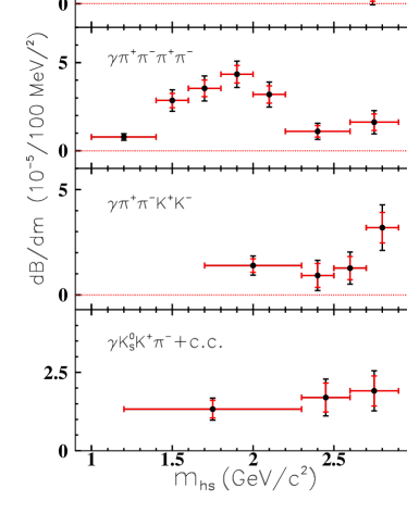
Figure 20: Differential branching fractions for $\psi(2S)$ decays into $\gamma p\overline{p}$, $\gamma 2(\pi^{+}\pi^{-})$, $\gamma K^{+}K^{-}\pi^{+}\pi^{-}$, and $\gamma K^{0}_{S}K^{+}\pi^{-}+c.c.$ Here $m_{hs}$ is the invariant mass of the hadrons in each final state. For each point, the smaller vertical error is the statistical error, while the bigger one is the sum of statistical and systematic errors.

Table 3 lists the results of $\psi(2S)$ decays into $\pi^{0}$ + hadrons together with the world averaged values PDG , and values of $Q_{h}~{}[={\cal B}(\psi(2S)\rightarrow h)/{\cal B}(J/\psi\rightarrow h)]$. For $\psi(2S)\rightarrow\pi^{0}2(\pi^{+}\pi^{-})$ decay, intermediate resonances including $\sigma~{}[f_{0}(600)]$, $f_{2}(1270)$, $\omega$, and $b_{1}(1235)$ are observed, and the measurement of ${\cal B}[\psi(2S)\rightarrow\omega f_{2}(1270)]$ agrees with the previous measurement using the same data sample bes2VP . The $\rho^{\pm}$ resonance is observed in $\psi(2S)\rightarrow\pi^{0}K^{0}_{S}K^{+}\pi^{-}+c.c.$ decay mode.

Table 2: Results for $\psi(2S)\rightarrow\gamma+hadrons$. For each final state, the following quantities are given: the number of events in $\psi(2S)$ data, $N^{Tot}$; the number of background events from $\psi(2S)$ decays and continuum, $N^{Bg}$; the number of signal events, $N^{Sig}$; and the weighted averaged efficiency, $\varepsilon$; the branching fraction with statistical and systematic errors or the upper limit on the branching fraction at the 90% C.L. For all the radiative channels, except the $\gamma p\overline{p}\pi^{0}$ and $\gamma\pi^{0}2(\pi^{+}\pi^{-})K^{+}K^{-}$ modes we require $m_{hs}<2.9~{}\mbox{GeV}/c^{2}$. The branching fraction for $\gamma\pi^{0}2(\pi^{+}\pi^{-})K^{+}K^{-}$ is measured with the requirement $m_{\pi^{0}2(\pi^{+}\pi^{-})K^{+}K^{-}}<3.38$ GeV/$c^{2}$. Possible interference effects for the modes with intermediate states are ignored.

Mode	$N^{Tot}$	$N^{Bg}$	$N^{Sig}$	$\varepsilon$(%)	${\cal B}(\times 10^{-5})$
$\gamma p\overline{p}$	$329$	$187$	$142\pm 18$	35.3	2.9$\pm$0.4$\pm$0.4
$\gamma p\overline{p}\pi^{0}$	$345$	$219$	$126\pm 38$	8.94	$10.1\pm 3.1\pm 2.1$
$\gamma 2(\pi^{+}\pi^{-})$	$1697$	$1114$	$583\pm 41$	10.4	39.6$\pm$2.8$\pm$5.0
$\gamma K^{0}_{S}K^{+}\pi^{-}+c.c.$	$-$	$-$	$115\pm 16$	4.83	25.6$\pm$3.6$\pm$3.6
$\gamma K^{+}K^{-}\pi^{+}\pi^{-}$	$361$	$229$	$132\pm 19$	4.94	19.1$\pm$2.7$\pm$4.3
$\gamma K^{*0}K^{+}\pi^{-}+c.c.$	$-$	$-$	$237\pm 39$	6.86	37.0$\pm$6.1$\pm$7.2
$\gamma K^{\ast 0}\overline{K}^{\ast 0}$	$58$	$17$	$41\pm 8$	2.75	24.0$\pm$4.5$\pm$5.0
$\gamma\pi^{+}\pi^{-}p\overline{p}$	$55$	$38$	$17\pm 7$	4.47	2.8$\pm$1.2$\pm$0.7
$\gamma 2(K^{+}K^{-})$	$15$	$8$	$<14$	2.93	$<4.0$
$\gamma 3(\pi^{+}\pi^{-})$	$118$	$95$	$<45$	1.97	$<17$
$\gamma 2(\pi^{+}\pi^{-})K^{+}K^{-}$	$17$	$13$	$<15.5$	0.69	$<22$
$\gamma\pi^{0}2(\pi^{+}\pi^{-})K^{+}K^{-}$	$27$	$21$	$<24.9$	$0.058$	$<310$

Table 3: Results of $\psi(2S)\rightarrow\pi^{0}+hadrons$. Here $N^{Sig}$ is the number of signal events, $\varepsilon$ is the detection efficiency, ${\cal B}$ is the measured branching fraction, ${\cal B}^{\textrm{PDG}}$ is the world averaged value PDG , and $Q_{h}={\cal B}(\psi(2S)\rightarrow h)/{\cal B}(J/\psi\rightarrow h)$. The branching fraction for $\pi^{0}2(\pi^{+}\pi^{-})K^{+}K^{-}$ is measured with the requirement $m_{2(\pi^{+}\pi^{-})K^{+}K^{-}}<3.38$ GeV/$c^{2}$.

Mode: $h$	$N^{Sig}$	$\varepsilon$(%)	${\cal B}(\times 10^{-4})$	${\cal B}^{\textrm{PDG}}(\times 10^{-4})$	$Q_{h}$(%)
$\pi^{0}2(\pi^{+}\pi^{-})$	$2173\pm 53$	$6.32$	$24.9\pm 0.7\pm 3.6$	$23.7\pm 2.6$	$10.5\pm 2.0$
$\omega\pi^{+}\pi^{-}$	$386\pm 23$	$3.74$	$8.4\pm 0.5\pm 1.2$	$6.6\pm 1.7$	$11.7\pm 2.4$
$\omega f_{2}(1270)$	$57\pm 13$	$3.65$	$2.3\pm 0.5\pm 0.4$	$2.0\pm 0.6$	$5.4\pm 0.6$
$b_{1}^{\pm}\pi^{\mp}$	$202\pm 21$	$3.24$	$5.1\pm 0.6\pm 0.8$	$3.6\pm 0.6$	$17.0\pm 4.2$
$p\overline{p}\pi^{0}\pi^{0}$	$203\pm 27$	8.30	$1.75\pm 0.21\pm 0.28$	—	—
$\pi^{0}K^{0}_{S}K^{\pm}\pi^{\mp}$	$361\pm 25$	4.40	$8.9\pm 0.6\pm 1.1$	—	—
$K^{\pm}\rho^{\mp}K^{0}_{S}$	$100\pm 20$	3.80	$2.9\pm 0.6\pm 0.4$	—	—
$\pi^{0}2(\pi^{+}\pi^{-})K^{+}K^{-}$	$48\pm 11$	$0.41$	$8.4\pm 1.9\pm 1.7$	—	—

In summary, we report measurements of the branching fractions of $\psi(2S)$ decays into $\gamma p\overline{p}$, $\gamma 2(\pi^{+}\pi^{-})$, $\gamma K^{0}_{S}K^{+}\pi^{-}+c.c.$, $\gamma K^{+}K^{-}\pi^{+}\pi^{-}$, $\gamma K^{\ast 0}K^{-}\pi^{+}+c.c.$, $\gamma K^{\ast 0}\overline{K}^{\ast 0}$, $\gamma\pi^{+}\pi^{-}p\overline{p}$, $\gamma 2(K^{+}K^{-})$, $\gamma 3(\pi^{+}\pi^{-})$, $\gamma 2(\pi^{+}\pi^{-})K^{+}K^{-}$ and the differential branching fractions for $\psi(2S)$ decays into $\gamma p\overline{p}$, $\gamma 2(\pi^{+}\pi^{-})$, $\gamma K^{+}K^{-}\pi^{+}\pi^{-}$, and $\gamma K^{0}_{S}K^{+}\pi^{-}+c.c.$ with hadron invariant mass less than 2.9$~{}\mbox{GeV}/c^{2}$. We also report branching fractions of $\psi(2S)$ decays into $\gamma p\overline{p}\pi^{0}$, $p\overline{p}\pi^{0}\pi^{0}$, $\pi^{0}K^{0}_{S}K^{+}\pi^{-}+c.c.$, $K^{\pm}\rho^{\mp}K^{0}_{S}$, $\pi^{0}2(\pi^{+}\pi^{-})K^{+}K^{-}$ and $\gamma\pi^{0}2(\pi^{+}\pi^{-})K^{+}K^{-}$. The measurements of $\psi(2S)$ decays into $\pi^{0}2(\pi^{+}\pi^{-})$, $\omega\pi^{+}\pi^{-}$, $\omega f_{2}(1270)$, and $b_{1}^{\pm}\pi^{\mp}$ are consistent with previous measurements PDG and the recent measurements by the CLEO collaboration chic23hs .

References

(1) L. Kpke and N. Wermes,
Phys. Rep. 174, 67 (1989).
(2) N. Brambilla et al., hep-ph/0412158.
(3)W.-M. Yao et al., Journal of Physics G 33, 1 (2006).
(4) P. Wang, C. Z. Yuan, and X. H. Mo, Phys. Rev. D 70, 114014 (2004).
(5) BES Collaboration, M. Ablikim et al., Phys. Rev.
Lett. 99, 011802 (2007).
(6) BES Collaboration, J. Z. Bai et al., Nucl. Instr. Meth.
A 344, 319 (1994).
(7)BES Collaboration, J. Z. Bai et al., Nucl. Instr. Meth. A 458, 627 (2001).
(8) X. H. Mo et al., HEP&NP 28, 455 (2004) [arXiv:hep-ex/0407055].
(9) S. P. Chi et al., HEP & NP 28, 1135 (2004).
(10)BES Collaboration, M. Ablikim et al.,
Nucl. Instrum. Meth. A 552, 344 (2005).
(11) J. C. Chen et al., Phys. Rev. D 62, 034003 (2000).
(12) R. G. Ping et al., HEP & NP 31, 229 (2007)
[arXiv:physics/0608213].
(13)BES Collaboration, M. Ablikim et al., Phys. Rev. D 71, 072006 (2005).
(14)BES Collaboration, M. Ablikim et al., Phys. Rev. Lett. 91, 022001 (2003).
(15) The mass resolution in
the fitted region is less than and neglected
in the fit.
(16) D. Aston et al., Nucl. Phys. B 296, 493 (1988).
(17) CLEO Collaboration, R. A. Briere et al., Phys. Rev. Lett. 95, 062001 (2005).
(18) J. Conrad, O. Botner, A. Hallgren, and C. Perez de los Heros, Phys. Rev. D 67, 012002 (2003).
(19) DM2 Collaboration, D. Bisello et al., Phys. Rev. D 39, 701 (1989);
MARK-III Collaboration, R. M. Baltrusaitis et al., Phys. Rev. D
33, 1222 (1986).
(20) This value includes the decays of
, ; the
intermediate resonance channels, e.g. are excluded.
(21) BES Collaboration, M. Ablikim et al., Phys. Rev. D 69, 072001 (2004).