Density oscillations in a model of water and other similar liquids

Abstract

It is suggested that the dynamics of liquid water has a component consisting of $O^{-2z}$ (oxygen) anions and $H^{+z}$ (hydrogen) cations, where $z$ is a (small) reduced effective electron charge. Such a model may apply to other similar liquids. The eigenmodes of density oscillations are derived for such a two-species ionic plasma, included the sound waves, and the dielectric function is calculated. The plasmons may contribute to the elementary excitations in a model introduced recently for the thermodynamics of liquids. It is shown that the sound anomaly in water can be understood on the basis of this model. The results are generalized to an asymmetric short-range interaction between the ionic species as well as to a multi-component plasma, and the structure factor is calculated.

Introduction. As simple as it may appear, water is still a complex liquid involving various interactions as well as kinematic and dynamic correlations. It is widely agreed that the water molecule in liquid water preserves to some extent its integrity, especially the directionality of the $sp^{3}$-oxygen orbitals, though it may be affected substantially by hydrogen bonds. As such, it is conceived that water has a molecular electric moment, an intrinsic polarizability and hindered rotations (librations) which may affect its orientational polarizability. We examine herein another possible component of the dynamics of the liquid water, as resulting from the dissociation of water molecule.

Water molecule $H_{2}O$ has two $H-O$ (hydrogen-oxygen) bonds which make an angle of cca $109^{\circ}$ in accordance with the tetragonal symmetry of the four hybridized $sp^{3}$-oxygen orbitals. The "spherical" diameter of water molecule is approximately $2.75\textrm{\AA}$ and the inter-molecular spacing in liquid water under normal conditions is $a\sim 3\textrm{\AA}$. This suggests that water molecule in liquid water, while preserving the directionality of the oxygen electronic orbitals, might be dissociated to a great extent. Dissociation models which assume $OH^{-}-H^{+}$ or $OH^{-}-H_{3}O^{+}$ pairs are known for water. This indicates a certain mobility of hydrogens (and oxygens). We analyze herein the hypothesis that water may consist of $O^{-2z}$ anions of mass $M=16amu$ and density $n$ and $H^{+z}$ cations (protons) of mass $m=1amu$ and density $2n$, where $z$ is a small reduced effective electron charge (the atomic mass unit is $1amu\simeq 1.7\times 10^{-24}g.$). We shall see that such a hypothesis adds another dimension to the dynamics of water. Such a model may apply to other similar liquids.

Due to their large mass the ions have a classical dynamics. Herein, we limit ourselves to considering the ions motion in water under the action of the Coulomb potentials $\varphi_{OO}=4z^{2}e^{2}/r$, $\varphi_{HH}=z^{2}e^{2}/r$ and $\varphi_{OH}=-2z^{2}e^{2}/r$, where $-e$ ($\simeq-4.8\times 10^{-10}esu$) is the electron charge and $r$ denotes the distance between the ions. For stability, it is necessary also to introduce a short-range repulsive (hard-core) potential $\chi$. It is shown that in the limit $z\rightarrow 0$ water may exhibit an anomalous sound-like mode beside both the ordinary (hydrodynamic) one and the non-equilibrium sound-like excitations governed by short-range interactions. We compute the density oscillations for this model, the dielectric function, the structure factor, and extend the model to a multicomponent plasma, including an asymmetric short-range interaction between ion species.

Plasmons in a jellium model. Let us consider one species of charged particles, with charge $-ze$, continuously distributed with density $n$ in a neutralising rigid continuous background of positive charge. This is the well-known jellium model. The Coulomb interaction reads

$$U=\frac{1}{2}\int d\mathbf{r}d\mathbf{r}^{\prime}\varphi(\mathbf{r}-\mathbf{r}^{\prime})\delta n(\mathbf{r})\delta n(\mathbf{r}^{\prime})\,\,\,,$$ (1)

where $\delta n(\mathbf{r})$ denotes a small disturbance of density (which preserves the global neutrality). We introduce the Fourier representation

$$\delta n(\mathbf{r})=\frac{1}{\sqrt{N}}\sum_{\mathbf{q}}\delta n(\mathbf{q})e^{i\mathbf{qr}}\,\,\,,\,\,\,\delta n(\mathbf{q})=\frac{n}{\sqrt{N}}\int d\mathbf{r}\delta n(\mathbf{r})e^{-i\mathbf{qr}}\,\,\,,$$ (2)

where $N=nV$ is the total number of particles in volume $V$. Similarly,

$$\varphi(\mathbf{r})=\frac{1}{V}\sum_{\mathbf{q}}\varphi(\mathbf{q})e^{i\mathbf{qr}}\,\,\,,\,\,\,\varphi(\mathbf{q})=\int d\mathbf{r}\varphi(\mathbf{r})e^{-i\mathbf{qr}}\,\,\,,$$ (3)

where $\varphi(\mathbf{q})=4\pi z^{2}e^{2}/q^{2}$ is the Fourier transform of the Coulomb potential (interaction). The Coulomb interaction given by (1) becomes

$$U=\frac{1}{2n}\sum_{\mathbf{q}}\varphi(q)\delta n(\mathbf{q})\delta n(-\mathbf{q})\,\,\,$$ (4)

(where the $q=0$-term is excluded by the positive background).

The small variations $\delta n(\mathbf{r})$ in density can be represented as $\delta n=-ndiv\mathbf{u}$, where $\mathbf{u}$ is a displacement vector. We emphasize that such a representation holds for $\mathbf{qu}(\mathbf{r})\ll 1$. It follows $\delta n(\mathbf{q})=-in\mathbf{q}\mathbf{u(}\mathbf{q})$, and one can see that the Coulomb interaction involves only longitudinal components of the displacement vector $\mathbf{u}(\mathbf{q})$ along the wavevector $\mathbf{q}$. Therefore, we may write $\mathbf{u}(\mathbf{q})=(\mathbf{q}/q)u(\mathbf{q})$, with $\delta n^{*}(-\mathbf{q})=\delta n(\mathbf{q})$, $\mathbf{\mathbf{u^{*}(-}q)\mathbf{=}u(}\mathbf{q})$ and $u^{*}(-\mathbf{q})=-u(\mathbf{q})$. The Coulomb interaction (4) becomes

$$U=-\frac{n}{2}\sum_{\mathbf{q}}q^{2}\varphi(q)u(\mathbf{q})u(-\mathbf{q})\,\,.$$ (5)

The kinetic energy associated with the coordinates $u(\mathbf{q})$ is given by

$$T=\frac{1}{2}\int d\mathbf{r}nm\dot{\mathbf{u}}^{2}=-\frac{1}{2}m\sum_{\mathbf{q}}\dot{u}(\mathbf{q})\dot{u}(-\mathbf{q})\,\,\,,$$ (6)

where $m$ denotes the particle mass. The equations of motion obtained from the Lagrange function $L=T-U$ are

$$m\ddot{u}(\mathbf{q})+nq^{2}\varphi(q)u(\mathbf{q})=0\,\,\,,$$ (7)

which leads to the well-known plasma oscillations with frequency given by $\omega_{p}^{2}=4\pi nz^{2}e^{2}/m$.

Plasma oscillations with two species of ions. We apply the above model to the two species of ions $O^{-2z}$ and $H^{+z}$. The change in density is associated with a displacement vector $\mathbf{v}$ in the former and a displacement vector $\mathbf{u}$ in the latter. First we note that the Fourier transforms of the Coulomb potentials are given by $\varphi_{OO}=4\varphi(q)$, $\varphi_{HH}=\varphi(q)$ and $\varphi_{OH}=-2\varphi(q)$, where $\varphi(q)=4\pi z^{2}e^{2}/q^{2}$. Therefore, the interactions can be written as

$$\begin{array}[]{c}U_{OO}=-\frac{n}{2}\sum_{\mathbf{q}}q^{2}\left[4\varphi(q)+\chi(q)\right]v(\mathbf{q})v(-\mathbf{q})\,\,\,,\\ \\ U_{HH}=-2n\sum_{\mathbf{q}}q^{2}\left[\varphi(q)+\chi(q)\right]u(\mathbf{q})u(-\mathbf{q})\,\,\,,\\ \\ U_{OH}=n\sum_{\mathbf{q}}q^{2}[2\varphi(q)-\chi]u(\mathbf{q})v(-\mathbf{q})\,\,\,,\end{array}$$ (8)

where $n=N/V$ is the density of water molecules and the Fourier transform $\chi$ of a hard-core potential has been introduced (the same for both species). The kinetic energy is given by

$$T=-\frac{1}{2}M\sum_{\mathbf{q}}\dot{v}(\mathbf{q})\dot{v}(-\mathbf{q})-m\sum_{\mathbf{q}}\dot{u}(\mathbf{q})\dot{u}(-\mathbf{q})\,\,\,,.$$ (9)

and the equations of motion read

$$\begin{array}[]{c}m\ddot{u}+2nq^{2}(\varphi+\chi)u-nq^{2}(2\varphi-\chi)v=0\\ \\ M\ddot{v}+nq^{2}(4\varphi+\chi)v-2nq^{2}(2\varphi-\chi)u=0\,\,\,,\end{array}$$ (10)

where we have dropped out the argument $\mathbf{q}$.

The solutions of these equations can be obtained straightforwardly. In the long wavelength limit $\mathbf{q}\rightarrow 0$ there are two branches of eigenfrequencies, one given by

$$\omega_{p}^{2}=\frac{16\pi nz^{2}e^{2}}{\mu}\,\,\,$$ (11)

corresponding to plasma oscillations and another given by

$$\omega_{s}^{2}=\frac{9n\chi}{M+2m}q^{2}=v_{s}^{2}q^{2}\,\,\,$$ (12)

corresponding to sound-like waves propagating with velocity $v_{s}$ given by (12). $\mu=2mM/(2m+M)$ is the reduced mass. The plasma oscillations are associated with antiphase oscillations of the relative coordinate ($2mu+Mv=0$), while the sound waves are associated with in-phase oscillations of the center-of-mass coordinate ($u-v=0$).

Polarization. An external electric field arising from a potential $\phi(\mathbf{r})$ gives an additional energy

$$U_{i}=q_{i}\int d\mathbf{r}\phi(\mathbf{r})\delta n_{i}(\mathbf{r})=-i(n_{i}q_{i}/n)\sum_{\mathbf{q}}q\phi(\mathbf{q})u_{i}(-\mathbf{q})\,\,\,,$$ (13)

for a species of ions labelled by $i$, with electric charge $q_{i}$ and density $n_{i}$. We apply this formula to the two-species ionic plasma, and get

$$U_{H}=-2ize\sum_{\mathbf{q}}q\phi(\mathbf{q})u(-\mathbf{q})\,\,,\,\,U_{O}=2ize\sum_{\mathbf{q}}q\phi(\mathbf{q})v(-\mathbf{q})\,\,$$ (14)

Adding these two terms to the lagrangian, the equations of motion given by (10) become

$$\begin{array}[]{c}m\ddot{u}+2nq^{2}(\varphi+\chi)u-nq^{2}(2\varphi-\chi)v=-izeq\phi\\ \\ M\ddot{v}+nq^{2}(4\varphi+\chi)v-2nq^{2}(2\varphi-\chi)u=2izeq\phi\,\,\,,\end{array}$$ (15)

where we have dropped out the argument $\mathbf{q}$. This is a system of coupled harmonic oscillators under the action of an external force. In the limit of long wavelengths its solutions are given by

$$\begin{array}[]{c}u=\frac{izeq}{m}\phi\frac{\omega^{2}-\frac{2m}{3\mu}\omega_{s}^{2}}{(\omega^{2}-\omega_{p}^{2})(\omega^{2}-\omega_{s}^{2})}\,\,\,,\\ \\ v=-\frac{2izeq}{M}\phi\frac{\omega^{2}-\frac{2M}{3\mu}\omega_{s}^{2}}{(\omega^{2}-\omega_{p}^{2})(\omega^{2}-\omega_{s}^{2})}\,\,.\end{array}$$ (16)

On the other hand, equation $n_{i}div\mathbf{u}_{i}=-\delta n_{i}$ is in fact the Maxwell equation $div\mathbf{E}_{i}=4\pi q_{i}\delta n_{i}$, where the electric field is given by $\mathbf{E}_{i}=-4\pi nq_{i}\mathbf{u}_{i}$. We have therefore the internal electric fields $E_{u}=-8\pi nzeu$ and $E_{v}=8\pi nzev$. The polarization $P=-(E_{u}+E_{v})/4\pi$ is given by

$$P(\mathbf{q})=2nze\left[u(\mathbf{q})-v(\mathbf{q})\right]=\frac{iq}{4\pi}\phi(\mathbf{q})\frac{\omega_{p}^{2}}{\omega^{2}-\omega_{p}^{2}}\,\,.$$ (17)

The external field is related to the external potential through $D(\mathbf{q})=-iq\phi(\mathbf{q})$ and the dielectric function $\varepsilon$ is given by $D=\varepsilon E=\varepsilon(D+E_{int})$, where $E_{int}=E_{u}+E_{v}$ is the internal field. We get the dielectric function

$$\varepsilon=1-\omega_{p}^{2}/\omega^{2}\,\,\,,$$ (18)

as expected. As it is well-known, its zero gives the longitudinal mode of plasma oscillations.

The $\omega_{p}$ in the nominator of equation (18) defines also the plasma edge: for frequencies lower than $\omega_{p}$ the electromagnetic waves are absorbed (the refractive index is given by $n^{2}=\varepsilon$). It is well-known that water exhibits indeed a strong absorption in the gigahertz-terrahertz region. On the other hand, neutron scattering on heavy water, as well as inelastic $X$-ray scattering, revealed the existence of a dispersionless mode $\simeq 4-5meV$ ($\simeq 10^{13}s^{-1}$) in the structure factor, which may be taken tentatively as the $\omega_{p}$-plasmonic mode given by equation (11). Making use of this equation we get $\omega_{p}\simeq 3\times 10^{14}zs^{-1}$($n=1/a^{3},$ $a=3\textrm{\AA}$), so we may estimate the reduced effective charge $z\simeq 3\times 10^{-2}$.

Dielectric function. The dielectric function given by equation (18) has a singularity for $\omega=0$, as arising from the exact cancellation in the static limit of the external field by the internal field. It is plausible to assume that residual polarization fields are still present in this static limit, like, for instance, the intrinsic polarizability. In this case, equation (18) is modified, and the dielectric function is of the type

$$\varepsilon=\frac{\omega^{2}-\omega_{p}^{2}}{\omega^{2}+\omega_{0}^{2}}\,\,\,,$$ (19)

where $\omega_{0}$ is a plasma frequency associated with the intrinsic, molecular polarizability. As such, it is a very high frequency, and equation (19) gives a small, negative contribution to the dielectric function in the static limit ($\omega\rightarrow 0$).

The dielectric properties of water are still a matter of debate. It is agreed that the permitivity dispersion of water is described to some extent by a Debye model of the form $\varepsilon=a+b/(1-i\omega\tau)$, where $a$ and $b$ are semi-empirical parameters and $\tau\sim\eta a^{3}/T$ is a relaxation time; $\eta$ denotes the viscosity and $T$ is the temperature. This Debye model assumes mainly an orientational polarizability of electric dipoles, which, due to the preservation of the directional character of the $O-H$ bonds, is compatible with the plasma model suggested here for water. Therefore, the contribution given by equation (19) should be added to the above Debye formula for the dielectric function, which becomes

$$\varepsilon=a+\frac{b}{1-i\omega\tau}+\frac{\omega^{2}-\omega_{p}^{2}}{\omega^{2}+\omega_{0}^{2}}\,\,.$$ (20)

Parameters $a$ and $b$ in equation (20) are related to the static permitivity $\varepsilon_{0}$ and high-frequency permitivity $\varepsilon_{\infty}$ through

$$\varepsilon_{0}=a+b-\omega_{p}^{2}/\omega_{0}^{2}\,\,,\,\,\varepsilon_{\infty}=a+1\,\,.$$ (21)

We may neglect $\omega_{p}^{2}/\omega_{0}^{2}$ here because it is too small, and we may also take $\varepsilon_{\infty}=1$($a=0$). The static permitivity $\varepsilon_{0}=b$ is given mainly by the electric dipoles. Let $\mathbf{p}$ be such an electric dipole. Its energy in an electric field $\mathbf{D}$ is $-pD\cos\theta$, where $\theta$ is the angle between $\mathbf{p}$ and $\mathbf{D}$. The thermal distribution of such dipoles is $dw\sim\exp(-pD\cos\theta/T)d(\cos\theta),.$where $T$ denotes the temperature. We get easily the thermal average $\left\langle\cos\theta\right\rangle=-L(pD/T)$, where $L(x)=\coth x-1/x$ is the well-known Langevin’s function.

We take $p=2ez_{e}(a/2)=ez_{e}a$, where $a\sim 3\textrm{\AA}$ and $z_{e}$ is a delocalized reduced charge associated with the $H-O$ dipole. We estimate the argument $pD/T$ of the Langevin’s function. At room temperature, we find $pD/T\simeq 3\times 10^{-4}Dz_{e}$. For $pD/T=1$ this corresponds to an external field $D=\frac{1}{3z_{e}}\times 10^{4}esu$, or $D=10^{8}/z_{e}V/m$. This is an extremely high field, so we are justified to take $pD/T\ll 1$, and $L(pD/T)\simeq pD/3T$. We get therefore a polarization $P=-np\left\langle\cos\theta\right\rangle=np^{2}D/3T$, an internal field $E_{int}=-4\pi P=-4\pi np^{2}D/3T$, and a permitivity

$$\varepsilon_{0}=b=\frac{1}{1-4\pi np^{2}/3T}\,\,\,$$ (22)

from $D=\varepsilon E=\varepsilon(D+E_{int})$. This is the well-known Kirkwood formula. For the empirical value $\varepsilon_{0}=80$, we get (at room temperature) a reduced charge $z_{e}\simeq 10^{-2}$. This is in good agreement with the $H^{+z}-O^{-2z}$ plasma charge $z$ estimated above.

Cohesion and thermodynamics. Recently, a model of liquid has been introduced based on an excitation spectrum (per particle) of the form $\varepsilon_{n}=-\varepsilon_{0}+\varepsilon_{1}(n+1/2)$, where $\varepsilon_{0}$ is a cohesion energy and $\varepsilon_{1}$ is the quanta of energy of a harmonic oscillator with one degree of freedom; $n$ represents here the quantum number. The model includes also the kinematic correlations (spatial restrictions) of the movement of the liquid molecules. This model leads to a consistent thermodynamics for liquids, arising from a statistics which is equivalent with the statistics of bosons in two dimensions.

For water, the cohesion energy per particle $\varepsilon_{0}$ can be estimated from the vaporization heat ($\simeq 40kJ/mol$). It gives $\varepsilon_{0}\sim 10^{3}K$. On the other hand, it was shown in a previous paper that the transition temperature beween a gas and a liquid of identical particles is approximately given by

$$T_{t}=\frac{4}{3}\frac{\varepsilon_{0}}{\ln(\varepsilon_{0}/T_{0})}\,\,\,,$$ (23)

where $T_{0}=\hbar^{2}n^{2/3}/m$ is a gas characteristic temperature. We can apply this formula to water disssociation, taking $n$ as the density of hydrogen atoms, $m$ as the mass of two hydrogen atoms and $T_{t}=383K$ (at normal pressure; $\varepsilon_{0}$ depends on the inter-particle spacing). We may neglect the oxygen, as it is too heavy in comparison with the hydrogen atoms. We get $T_{0}\simeq 2K$ and the above formula gives $\varepsilon_{0}\simeq 2000K\simeq 200meV$ for the cohesion energy of water per molecule, which is consistent with the above estimate ($1eV\simeq 11.6\times 10^{3}K$; $n\simeq 1/a^{3}$ with $a=3\textrm{\AA}$ and $\hbar\simeq 10^{-27}erg\cdot s$; Bohr radius $a_{H}=\hbar^{2}/m_{e}e^{2}\simeq 0.53\textrm{\AA}$, $e^{2}/a_{H}\simeq 27.2eV$, where $m_{e}$ is the electron mass).

The plasma oscillations obtained above can be quantized and the energy levels of the plasma read

$$E_{n}=\sum_{\mathbf{q}}\hbar\omega_{p}(n+1/2)=\frac{V}{(2\pi)^{3}}\frac{4\pi}{3}q_{c}^{3}\cdot\hbar\omega_{p}(n+1/2)\,\,\,,$$ (24)

where $q_{c}$ is a cutoff wavevector. The prefactor in equation (24) is $Vq_{c}^{3}/6\pi^{2}\simeq N(aq_{c}/4)^{3}$, so the energy levels given above can be written as

$$E_{n}=N\varepsilon_{1}(n+1/2)\,\,\,,$$ (25)

where $\varepsilon_{1}=(aq_{c}/4)\hbar\omega_{p}$. These energy levels correspond to a harmonic oscillator with one degree of freeedom. It follows that the present description of water as a two-species of highly dissociated ionic plasma provides a further support for the liquid model mentioned above. If we take $q_{c}\simeq 1/a$ the energy quanta $\varepsilon_{1}=(aq_{c}/4)^{3}\hbar\omega_{p}=\simeq 3zmeV$ represents the $\varepsilon_{1}$ parameter in the spectrum of the liquid. (The plasma frequency given by equation (11) is $\omega_{p}\simeq 200zmeV$).

Debye screening and the correlation energy. As it is well-known the plasma excitations described above represent collective oscillations of the density in the long wavelength limit. At the same time they induce correlations in the ionic movements. For a classical plasma these correlations are associated with a screening length given by the Debye-Huckel theory as

$$\kappa^{-1}=\left(T/24\pi nz^{2}e^{2}\right)^{1/2}\,\,\,$$ (26)

for our case ($\kappa^{-1}=\left(T/4\pi e^{2}\sum_{i}n_{i}z_{i}^{2}\right)^{-1}$where $i$ labels the ionic species with density $n_{i}$ and charge $ez_{i}$). The formula is valid for the Coulomb energy $z^{2}e^{2}/a$ much lower than the temperature $T$. In the present case we have $z^{2}e^{2}/a\simeq 45K$ (for $z\simeq 3\times 10^{-2}$), which shows that the above condition is fulfilled. From (26) we get $\kappa^{-1}\sim 1\textrm{\AA}$ (at room temperature), in agreement with the present molecular-dissociation model. The correlation energy per particle is given by

$$\varepsilon_{corr}=-\frac{e^{2}}{a}\sqrt{\frac{\pi e^{2}}{Ta}}(6z^{2})^{3/2}\,\,\,$$ (27)

($\varepsilon_{corr}=-(e^{2}/a)\sqrt{\pi e^{2}/Ta}(\sum_{i}n_{i}z_{i}^{2})^{3/2}$). The estimation of this energy gives $\varepsilon_{corr}\sim 10^{2}K$ (at room temperature). It contributes to the cohesion energy.

Sound anomaly. The sound-like branch $\omega_{2}\simeq\omega_{s}=v_{s}q$, where $v_{s}=\sqrt{9n\chi/(M+2m)}$ according to equation (12), is distinct from the ordinary hydrodynamic sound whose velocity is given by the well-known formula $v_{0}=1/\sqrt{\kappa nm}$ for a one-component fluid, where $\kappa$ is the adiabatic compressibility. For the present two-component fluid ($H^{+z}-O^{-2z}$ plasma), the velocity of the ordinary sound is given by $v_{0}=1/\sqrt{\kappa n(M+2m)}$. The former represents a non-equilibrium elementary excitation, whose velocity $v_{s}$ does not depend on temperature, while the latter proceeds by thermodynamic, equilibrium, adiabatic processes, and its velocity $v_{0}$ depends on temperature thorugh the adiabatic conpresibility $\kappa$. In order to distinguish them from the hydrodynamic sound we propose to call the sound-like excitations derived here density "kinetic" modes or "densitons". The distinction between the two sounds is made by a threshold wavevector $q_{t}$ in the following manner. Suppose that there is a finite lifetime $\tau$ for the sound-like excitations $\omega_{s}$ propagating with a velocity $v_{s}$ and a corresponding meanfree path $\Lambda=v_{s}\tau$. If the sound-like wavelength $\lambda$ is much longer than the meanfree path, $\lambda\gg\Lambda$, then we are in the collision-like regime ($\omega_{s}\tau\ll 1$), and the collisions may restore the thermodynamic equilibrium. In this case the hydrodynamic sound propagates, and the sound-like excitations do not. This condition defines the threshold wavevector $q_{t}=1/v_{s}\tau$. In the opposite case, $q\gg q_{t}$ (collision-less regime), it is the sound-like excitations that propagate, and not the hydrodynamic sound. The finite lifetime $\tau$ originates in the residual interactions between the collective modes and the underlying motion of the individual particles. It is easy to estimate this residual interaction. It is given by $\sqrt{\varepsilon T}$, where $\varepsilon$ is the mean energy per particle corresponding to the motion of the individual particles. We get therefore $\tau\simeq\hbar/\sqrt{\varepsilon T}$ and the threshold wavevector $q_{t}=\sqrt{\varepsilon T}/\hbar v_{s}$. It is difficult to have a reliable estimation of the mean energy $\varepsilon$; for a resonable value $\varepsilon=10meV$ we get $q_{t}\simeq 0.1\textrm{\AA}^{-1}$ at room temperature for $v=3000m/s$, which is in good agreement with experimental data.

Indeed, the phenomenon of two-sound anomaly in water is well-documented. Neutron, $X$-ray, Brillouin or ultraviolet light scattering on water revealed the existence of a hydrodynamic sound propagating with velocity $v_{0}\simeq 1500m/s$ for smaller wavevectors and an additional sound propagating with velocity $\simeq 3000m/s$ for larger wavevectors. In addition, though both sound velocities do exhibit an isotopic effect, their ratio does not. According to the above discussion, we assign this additional, faster sound to the sound-like excitations derived here. We can see that both $v_{0}$ and $v_{s}$ given above exhibit a weak isotopic effect, while their ratio $v_{s}/v_{0}=3n\sqrt{\kappa\chi}$ does not. From $v_{s}=\sqrt{9n\chi/(M+2m)}=3000m/s$ we get the short-range interaction $\chi\simeq 7eV\cdot\textrm{\AA}^{3}$. Similar results are obtained for other forms of dissociation of the water molecule, like $OH^{-}-H^{+}$ or $OH^{-}-H_{3}O^{+}$, so the $H^{+z}-O^{-2z}$ plasma model employed here can be viewed as an average, effective model for various plasma components that may exist in water.

Another possible anomalous sound. It is worth calculating the spectrum given by equations of motion (10) without neglecting higher-order contributions in $q^{2}$. The result of this calculation is given by

$$\omega_{1,2}^{2}=\frac{1}{2}\omega_{p}^{2}\left[1+Ax^{2}\pm\sqrt{1+2Bx^{2}+A^{2}x^{4}}\right]\,\,\,,$$ (28)

where

$$A=\frac{1}{9\alpha}(2+5\alpha+2\alpha^{2})\,\,,\,\,B=\frac{1}{9\alpha}(2-13\alpha+2\alpha^{2})\,\,,\,\,\alpha=m/M\,\,\,$$ (29)

and $x=v_{s}q/\omega_{p}$. It is shown in Fig. 1.

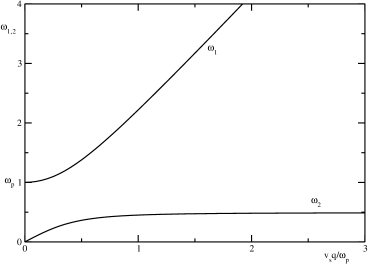
Figure 1: The spectrum of the density oscillations given by equation (28) for the $H^{+z}-O^{-2z}$ plasma with the same short-range interaction between ionic species.

Frequency $\omega_{2}$ in equation (28) represents the sound-like branch, which goes like $\omega_{2}\simeq\omega_{s}=v_{s}q$ in the long wavelength limit and approaches the horizontal asymptote $\omega_{2}=\omega_{p}/\sqrt{A}\simeq\omega_{p}\sqrt{m/2M}$ for shorter wavelengths. Frequency $\omega_{1}$ in equation (28) represents the plasmonic branch ($\omega_{1}\simeq\omega_{p}$ for $q\rightarrow 0$). In the long wavelength limit it goes like

$$\omega_{1}\simeq\omega_{p}+\frac{(M-m)^{2}}{9mM}v_{s}^{2}q^{2}/\omega_{p}\,\,\,,\,\,\,q\rightarrow 0\,\,.$$ (30)

Due to the large disparity between the two masses $m$ and $M$ we can see that the plasma frequency has an abrupt increase toward the short-wavelength oblique asymptote given by

$$\omega_{a}\simeq\sqrt{A}v_{s}q\simeq\sqrt{2M/9m+5/9}v_{s}q\,\,.$$ (31)

For small values of $\omega_{p}$ (vanishing Coulomb coupling, $z\rightarrow 0$) this asymptotic frequency may look like an anomalous sound propagating with velocity

$$v_{a}\simeq\sqrt{2M/9m+5/9}v_{s}\,\,.$$ (32)

For water, we get $v_{a}\simeq 2v_{s}$ from this formula. However, the ratios $v_{a}/v_{s}$ or $v_{a}/v_{0}$ exhibit a rather strong isotopic effect, which is not supported by experimental data.

Multi-component plasma. The model presented herein might be generalized to a multi-component plasma consisting of several ionic species labelled by $i$, each with number $N_{i}$ of particles, density $n_{i}$, charge $z_{i}e$ and mass $m_{i}$, such that $\sum_{i}z_{i}n_{i}=0$.

The lagrangian of the density oscillations is given by

$$\begin{array}[]{c}L=-\frac{1}{2n}\sum_{i\mathbf{q}}m_{i}n_{i}\dot{u}_{i}(\mathbf{q})\dot{u}_{i}(-\mathbf{q})+\frac{1}{2n}\sum_{ij\mathbf{q}}n_{i}n_{j}q^{2}\left[\varphi_{ij}(q)+\chi(q)\right]u_{i}(\mathbf{q})u_{j}(-\mathbf{q})+\\ \\ +i\frac{e}{n}\sum_{i\mathbf{q}}n_{i}z_{i}q\phi(\mathbf{q})u_{i}(-\mathbf{q})\,\,\,,\end{array}$$ (33)

where $\varphi_{ij}(q)=4\pi z_{i}z_{j}e^{2}/q^{2}$. The equations of motion are given by

$$m_{i}\ddot{u}_{i}+4\pi e^{2}z_{i}\sum_{j}z_{j}n_{j}u_{j}+q^{2}\chi\sum_{j}n_{j}u_{j}=-iqez_{i}\phi\,\,.$$ (34)

Making use of the notations

$$S_{1}=\sum_{i}z_{i}^{2}n_{i}/m_{i}\,\,,\,\,S_{2}=\sum_{i}n_{i}/m_{i}\,\,,\,\,S_{3}=\sum_{i}z_{i}n_{i}/m_{i}\,\,\,,$$ (35)

the eigenfrequencies $\omega_{1,2}$ of the system of equations (34) in the long wavelength limit are given by

$$\omega_{1}^{2}\simeq\omega_{p}^{2}=4\pi e^{2}S_{1}=\sum_{i}\frac{4\pi e^{2}z_{i}^{2}n_{i}}{m_{i}}\,\,\,,$$ (36)

which represents the plasma branch of the spectrum, and

$$\omega_{2}^{2}\simeq\omega_{s}^{2}=\left(S_{2}-S_{3}^{2}/S_{1}\right)\chi q^{2}=v_{s}^{2}q^{2}\,\,\,,$$ (37)

which represents the sound-like excitations. The plasma branch of the spectrum has an oblique asimptote given by $\omega_{1}\simeq\omega_{a}=\sqrt{\chi S_{2}}q$, which may be taken as an anomalous sound propagating with velocity $v_{a}=\sqrt{\chi S_{2}}$ for small values of $\omega_{p}$. The ratio of the two sound velocities is given by

$$v_{a}/v_{s}=\frac{1}{\sqrt{1-S_{3}^{2}/S_{1}S_{2}}}\,\,\,,$$ (38)

which is always higher than unity. The sound branch of the spectrum has an horizontal asymptote given by $\omega_{2}\simeq\sqrt{1-S_{3}^{2}/S_{1}S_{2}}\omega_{p}$. For the $H^{+z}-O^{-2z}$ plasma we can check from (38) that $v_{a}/v_{s}\simeq(2M/9m+5/9)^{1/2}\simeq 2$, and $\omega_{2}\simeq 3\sqrt{m/2M}\omega_{p}$, as obtained above. As we have discussed above this ratio exhibits a rather strong isotopic effect, which is not in accord with experimental data. We assign therefore the additional sound to sound-like excitations propagating with velocity $v_{s}$ given by equation (37). The ordinary, hydrodynamic sound in a multi-component mixture has the velocity $v_{0}=1/\sqrt{\kappa\sum_{i}n_{i}m_{i}}$. It can be shown that $v_{s}^{2}/v_{0}^{2}\geq n^{2}\kappa\chi$ for a neutral multi-component mixture.

The internal field is given by

$$E_{int}=-4\pi e\sum_{i}z_{i}n_{i}u_{i}\,\,\,;$$ (39)

we get easily from equations (34)

$$E_{int}=-iq\phi\frac{\omega_{p}^{2}}{\omega^{2}-\omega_{p}^{2}}\,\,\,$$ (40)

and the dielectric function $\varepsilon=1-\omega_{p}^{2}/\omega^{2}$, as expected.

Structure factor. The structure factor is defined by

$$\begin{array}[]{c}S(q,\omega)=\frac{1}{2\pi}\int d\mathbf{r}d\mathbf{r}^{\prime}dt\left\langle\delta n(\mathbf{r},t)\delta n(\mathbf{r}^{\prime},0)\right\rangle e^{i\mathbf{q}(\mathbf{r}-\mathbf{r}^{\prime})-i\omega t}=\\ \\ =\frac{N}{2\pi n^{2}}\int dt\left\langle\delta n(\mathbf{q},t)\delta n(-\mathbf{q},0)\right\rangle e^{-i\omega t}\,\,\,,\end{array}$$ (41)

where the brackets stand for the thermal average (we leave aside the central peak). Since

$$\delta n(\mathbf{q},t)=-iq\sum_{i}n_{i}u_{i}(\mathbf{q},t)\,\,\,,$$ (42)

it becomes

$$S(q,\omega)=\frac{Nq^{2}}{2\pi n^{2}}\int dt\sum_{ij}n_{i}n_{j}\left\langle u_{i}(t)u_{j}(0)\right\rangle e^{-i\omega t}\,\,\,,$$ (43)

where we dropped out the argument $\mathbf{q}$.

In order to calculate the thermal averages we turn back to the system of equations (34) without the external electric field. This system can be written as

$$\begin{array}[]{c}(-\omega^{2}+aS_{1})x+bS_{3}y=0\,\,\,,\\ \\ aS_{3}x+(-\omega^{2}+bS_{2})y=0\,\,\,,\end{array}$$ (44)

where $a=4\pi e^{2}$, $b=\chi q^{2}$, $S_{1,2,3}$ are given by equation (35) and

$$x=\frac{1}{n}\sum_{i}z_{i}n_{i}u_{i}\,\,\,,\,\,\,y=\frac{1}{n}\sum_{i}n_{i}u_{i}\,\,.$$ (45)

In addition,

$$u_{i}=\frac{anz_{i}}{m_{i}\omega^{2}}x+\frac{bn}{m_{i}\omega^{2}}y\,\,.$$ (46)

The system of equations (44) has two eigenfrequencies $\omega_{1,2}$ as given by equations (36) and (37). The corresponding eigenvectors are given by

$$x_{1}\sim S_{1}\,\,,\,\,y_{1}\sim S_{3}\,\,\,;\,\,\,x_{2}\sim bS_{3}\,\,,\,\,y_{2}\sim-aS_{1}\,\,\,$$ (47)

in the long wavelength limit. According to equation (46) the coordinates $u_{i}$ can be written as

$$u_{i}^{(1,2)}=\frac{anz_{i}}{m_{i}\omega_{1,2}^{2}}x_{1,2}e^{i\omega_{1,2}t}+\frac{bn}{m_{i}\omega_{1,2}^{2}}y_{1,2}e^{i\omega_{1,2}t}\,\,\,,$$ (48)

and one can see that they are coordinates of linear harmonic oscillators with frequencies $\omega_{1,2}$ and potential energies $m_{i}\omega_{1,2}^{2}\left[u_{i}^{(1,2)}\right]^{2}/2$ . The thermal distribution of the coordinate $u$ for such an oscillator is given by $dw=\sqrt{m\omega^{2}/2\pi T}\exp\left(-m\omega^{2}u^{2}/2T\right)du$ in the classsical limit, where $T$ denotes the temperature ($T\gg\hbar\omega$). It follows

$$\left\langle u_{i}^{(1,2)}u_{j}^{(1,2)}\right\rangle=\frac{T}{m_{i}\omega_{1,2}^{2}}\delta_{ij}\,\,.$$ (49)

Writing

$$u_{i}=u_{i}^{(1)}e^{i\omega_{1}t}+u_{i}^{(2)}e^{i\omega_{2}t}\,\,\,$$ (50)

and making use of equation (49) the structure factor given by equation (43) becomes

$$S(q,\omega)=NTq^{2}\left(\sum_{i}n_{i}^{2}/n^{2}m_{i}\right)\left[\frac{1}{\omega_{1}^{2}}\delta(\omega-\omega_{1})+\frac{1}{\omega_{2}^{2}}\delta(\omega-\omega_{2})\right]\,\,.$$ (51)

We can see from this equation that the relevant sound contributions are given by

$$S(q,\omega)\simeq\frac{NT}{v_{s,a}^{2}}\left(\sum_{i}n_{i}^{2}/n^{2}m_{i}\right)\delta(\omega-v_{s,a}q)\,\,.$$ (52)

Asymmetric short-range interaction. Up to now, the short-range interaction was assumed to be the same for all ionic species. In general, we may introduce a short-range interaction $\chi_{ij}$ depending on the nature of the ionic species. If this interaction is separable, the solution given above for a multi-component plasma holds with minor modifications. For a non-separable short-range interaction, appreciable changes may appear in the spectrum, which may exhibit multiple branches. Such a spectrum may serve to identify the nature (mass, charge) of various molecular aggregates in a multi-component plasma. It is worth noting that a range of frequencies $10^{10}s^{-1}-10^{12}s^{-1}$ is documented in living cells by microwave, Raman and optical spectroscopies and by cell-biology studies, upon which the theory of coherence domains in living matter is built.

We consider here again the $H^{+z}-O^{-2z}$ plasma with different short-range interaction $\chi_{HH}=\chi_{1\,,\,}\chi_{OO}=\chi_{2}\,,\,\chi_{OH}=\chi_{3}$; it still exhibits two branches of frequencies, a plasmonic one ($\omega_{1}$) and a sound-like one ($\omega_{2}$), but the spectrum may have certain peculiarities (the dielectric constant is not affected by this modification). Equations of motion (15) become now

$$\begin{array}[]{c}m\ddot{u}+2nq^{2}(\varphi+\chi_{1})u-nq^{2}(2\varphi-\chi_{3})v=-izeq\phi\\ \\ M\ddot{v}+nq^{2}(4\varphi+\chi_{2})v-2nq^{2}(2\varphi-\chi_{3})u=2izeq\phi\,\,.\end{array}$$ (53)

We introduce the notations

$$a=2nq^{2}\varphi/m=8\pi ne^{2}z^{2}/m\,\,\,,\,\,\,b_{1,2,3}=n\chi_{1,2,3}/m\,\,.$$ (54)

The dispersion relations can be computed straightforwardly. In the long wavelength limit ($q\rightarrow 0$) we get the plasmonic branch

$$\omega_{1}^{2}\simeq(1+2\alpha)a+\frac{2b_{1}+\alpha^{2}b_{2}-4\alpha b_{3}}{1+2\alpha}q^{2}\,\,\,,$$ (55)

where $(1+2\alpha)a=16\pi ne^{2}z^{2}/\mu$ is the plasma frequency, and the sound-like branch

$$\omega_{2}^{2}\simeq\frac{\alpha(4b_{1}+b_{2}+4b_{3})}{1+2\alpha}q^{2}=v_{s}^{2}q^{2}\,\,;$$ (56)

one can see that the sound velocity $v_{s}$ is always a real quantity.

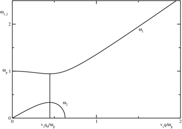
Figure 2: Excitation spectrum given by equation (59) for the $H^{+z}-O^{-2z}$ plasma with short-range potentials $\chi_{OO}=\chi_{HH}=0$ and $\chi_{OH}=\chi\neq 0$.

The sound-like branch exhibits an asymptote in the short-wavelength limit given by

$$\omega_{2}^{2}\sim\frac{1}{2}\left[2b_{1}+\alpha b_{2}-\sqrt{(2b_{1}-\alpha b_{2})^{2}+8\alpha b_{3}^{2}}\right]q^{2}\,\,\,,$$ (57)

whose slope may have either sign or vanish. It is easy to see that this slope is positive for $b_{3}^{2}<b_{1}b_{2}$, negative for $b_{3}^{2}>b_{1}b_{2}$ (when the sound-like branch has a maximum value) and it vanishes for $b_{3}^{2}=b_{1}b_{2}$ (when the sound-like branch has an horizontal asymptote). In the case of a negative slope the sound velocity may exhibit a negative velocity and the sound may suffer a strong absorption for moderate values of the wavevector, which may indicate an anomalous or unphysical situation.

We return now to the plasmon branch given by equation (55), and write it as

$$\omega_{1}^{2}=\omega_{p}^{2}+b_{2}\frac{2x^{2}-4\alpha\lambda x+\alpha^{2}}{1+2\alpha}q^{2}\,\,\,,$$ (58)

where $\lambda^{2}=b_{3}^{2}/b_{1}b_{2}$ and $x=\sqrt{b_{1}/b_{2}}.$ It is easy to see that for $\lambda^{2}>1$ the plasmonic spectrum exhibits a dip around a certain value $q_{0}$ of the wavevector $q$ for $\left(\lambda-\sqrt{\lambda^{2}-1/2}\right)\alpha<\sqrt{b_{1}/b_{2}}<\left(\lambda+\sqrt{\lambda^{2}-1/2}\right)\alpha$; it approaches an asymptote with a positive slope for $q\rightarrow\infty$, which may define again an anomalous sound for small values of $\omega_{p}$.

We illustrate these anomalies for a particular case of short-range interaction $\chi_{1,2}=0$ and $\chi_{3}=\chi$ ($b_{3}=n\chi/m$). The dispersion relations of the system of equations (53) become

$$\omega_{1,2}^{2}=\frac{1}{2}\omega_{p}^{2}\left[1\pm\sqrt{1-4v_{s}^{2}q^{2}/\omega_{p}^{2}+\frac{(1+2\alpha)^{2}}{2\alpha}v_{s}^{4}q^{4}/\omega_{p}^{4}}\right]\,\,.$$ (59)

The plasmonic branch has a minimum value for $q_{0}\simeq 2\sqrt{m/M}\omega_{p}/v_{s}$, where the sound-like branch has a maximum value ($\simeq\sqrt{2m/M}\omega_{p}$). The spectrum is shown in Fig. 2. Using $\omega_{p}\simeq 10^{13}s^{-1}$ estimated above and the sound velocity $v_{s}\simeq 3000m/s$ in water we get $q_{0}^{-1}\simeq 6\textrm{\AA}$. We may expand $\omega_{1}$ in series of $(q-q_{0})^{2}$ around its mimimum value at $q_{0}$ and get $\omega_{1}\simeq\omega_{p}+(M/4m+1)(v_{s}^{4}q_{0}^{2}/\omega_{p}^{3})(q-q_{0})^{2}=\omega_{p}+(1+4m/M)v_{s}^{2}(q-q_{0})^{2}/\omega_{p}$. This is similar with the rotons-like dispersion relation discussed in connection with the coherence domains in water. Although this might be an interesting suggestion, it is inconsequential here, because $\omega_{p}$ is too small in comparison with the temperatures at which water exists and, therefore, this "dip" feature has no effect for the water thermodynamics.

Conclusion. We summarize the main features of the model suggested here for liquid water. First, we assume, as it is generally accepted, the four, directional $sp^{3}$-oxygen electronic orbitals. The electron delocalization along two such orbitals together with a corresponding delocalization of the hydrogen electronic charge lead to the water cohesion. It is represented by the cohesion energy $\varepsilon_{0}$ discussed here. Within such a picture, we can still visualize the oxygen and the hydrogen as neutral atoms, moving around almost freely (as a consequence of the uniformity of the environment; this gives a noteworthy support to the "hydrogen bonds" concept). To this picture the present model adds another component, arising from a very small charge transfer between hydrogen and oxygen atoms, leading to a $H^{+z}-O^{-2z}$ plasma, with the reduced charge $z$. It may originate in the weak asymmetry of the two occupied $sp^{3}$-oxygen electronic orbitals with respect to the other two unoccupied orbitals. Under these circumstances, the hydrogen and oxygen ions interact, both by Coulomb and short-range potentials. This interaction gives the plasma frequency and the sound-like excitations frequency. The plasmons contribute to the excitations which give rise to a consistent thermodynamics for liquids, in a model introduced recently. In addition, the ionic plasma oscillations entail oscillations of the delocalized electronic cloud, with the same eigenfrequency. Subjected to an external field, these electronic oscillations produce an intrinsic polarizability which removes the $\omega=0$ singularity in the plasma dielectric function (the $\omega_{0}$ frequency). In addition, the magnitude of the electric moment $\mathbf{p}$ which is responsible for the orientational, static dielectric function is in satisfactory agrement with the plasma charge $z$ derived herein.

On the basis of this model we are able to understand to some extent, both qualitatively and in some places even quantitatively, the sound anomaly, the dielectric function (permitivity dispersion), the structure factor, cohesion and thermodynamics of water. The model is extended to a multi-component classical plasma, including an asymmetric short-range interaction between the components, which might be relevant for more complex structural aggregates like those in biological matter.