Stability of Quantized Vortices in a Bose-Einstein condensate confined in an Optical Lattice

Abstract

We investigate the existence and especially the linear stability of single and multiple-charge quantized vortex states of nonlinear Schrödinger equations in the presence of a periodic and a parabolic potential in two spatial dimensions. The study is motivated by the examination of pancake-shaped Bose-Einstein condensates in the presence of magnetic and optical confinement. A two-parameter space of the condensate’s chemical potential versus the periodic potential’s strength is scanned for both single- and double-quantized vortex states located at a local minimum or a local maximum of the lattice. Triply charged vortices are also briefly discussed. Single-charged vortices are found to be stable for cosinusoidal potentials and unstable for sinusoidal ones above a critical strength. Higher charge vortices are more unstable for both types of potentials and their dynamical evolution leads to breakup into single-charged vortices.

I Introduction

In the past decade, the study of coherent structures with topological charge has become increasingly popular in Hamiltonian systems. This has been especially so due to the emergence of both nonlinear optical, as well as atomic physics settings where such studies were experimentally relevant. Recent reviews both in the framework of optical fibers and waveguides desyatnikov , as well as in that of Bose-Einstein condensates (BECs) fetter ; us have given overviews of this rapidly growing area of research; see also Pismen . It is particularly interesting that both of these directions are associated with the prototypical dispersive equation that supports such structures, namely the nonlinear Schrödinger equation sulem .

More specifically, in the context of dilute alkali vapors forming BECs at extremely low temperatures, the experimental realization of one as well as a few vortices dalib1 ; cornell1 , followed by the realization of very robust vortex lattices kett1 has had a profound influence on the field. More recently, experimental efforts have turned to higher-charged vortices, illustrating not only how vortices of topological charge $S=2$ and even $S=4$ can be imprinted kett2 , but also the dynamical instability of such waves kett3 .

These experimental works have caused an intense theoretical interest in the existence and stability of vortices, especially under the case of parabolic confinement which is customary in BECs due to magnetic trapping. While vortices of topological charge $S=1$ were found to be stable in a parabolic potential, higher topological charges were found to be unstable. The work of pu illustrated the potential instability (for appropriate values of the number of atoms i.e., the spatially integrated square modulus of the solution) of $S=2$ and $S=3$ waveforms. Later, the work of kawa shed light into the case of $S=4$ and the role of negative energy eigenmodes in the instability. The studies of motto and ueda examined the various scenaria of split-up of higher charge vortices during dynamical evolution simulations for repulsive and attractive interactions (i.e., defocusing and focusing nonlinear Schrödinger equations) respectively. The work of carr examined such vortices riding on the background of not just the ground state, but also of higher, ring-like, excited states of the system. In the context of an optical lattice, the authors of borissak tried to construct both higher charge vortices, and super-vortices for attractive condensates in optical lattices, while in the repulsive setting the so-called gap vortices have been predicted ostr1 and systematically created ostr2 . More recently, these notions have also been examined from a more mathematically rigorous point of view, using tools such as the Evans function to compute the eigenvalue spectrum kollar , or weak perturbations from the linear limit, to obtain a full count on the potentially unstable eigenvalues todd .

One essential limitation of almost all of the above studies regarding the existence and stability of the vortices has been the radial nature of the symmetry of the parabolically confined system. In that radially symmetric setting, the authors of the above theoretical references proceeded to convert the problem to an effectively one-dimensional one along the radial direction, which it is straightforward to solve by a shooting method or otherwise. Then, when the so-called Bogolyubov-de Gennes (or linear stability) analysis was performed around the ensuing radial excitations, the radial symmetry was again crucially involved, as the angular dependence of the perturbation modes was decomposed into Fourier modes, resulting into a one-parameter infinity of radial problems (indexed by the wavenumber of the angular mode); for the mathematical details of this analysis see e.g., pegowar . As discussed in pegowar , subsequent examination of only the lower modes in the resulting quasi-1d stability problem is sufficient to extract conclusions on the stability of the full 2d radial state. It should be mentioned in passing that the more recent works of lundh1 ; lundh2 considered the stability of multiply quantized vortices in three-dimensional BECs.

This above radial approach, however, does not allow us to examine the stability of states in the presence of both a magnetic trap and an optical lattice. In the latter setting, the combined potential breaks the radial symmetry and defies any one-dimensional approach towards the identification of the solutions or of their stability. In view of that, while numerous works examine the existence and linear stability of states in the presence of the parabolic trap, references that address the properties of the vortices in combined potentials are scant; in fact, we are only aware of the direct integration results of pgk which illustrate the disparity of the effects of the optical lattice phase on vortices of $S=1$, and of the entirely theoretical work of bhatta that calculated the normal modes of the system based on a Lagrangian approach.

Our purpose in the present work is to examine systematically both the existence and the stability of both single-charged as well as multiply charged vortices in the presence of the combined parabolic and periodic potentials. The considerable numerical load that is required to perform the relevant computations (and which, we believe, is what prevented an earlier study of this topic) is circumvented with two separate variations of Newton’s method which both allow us to perform equally efficient fixed point iteration that converges on numerically exact solutions of the system. The variations differ in the method of handling the linear system in each Newton iteration, which is far beyond the capacity of a standard direct linear solvers. One scheme implements an iterative linear solver in each Newton step, and the other implements a standard sparse banded matrix solver. We subsequently critically use the sparse nature of the relevant stability matrices to invoke a sparse Arnoldi iterative algorithm for approximating the system’s eigenvalues, which, in turn, allows us to determine the linear stability (i.e., to computationally perform the Bogolyubov-de Gennes analysis) of the resulting vortices. This permits us to develop two-parameter diagrams (as a function of the chemical potential, and of the strength of the periodic potential) for the existence and stability of solutions with $S=1$ and $S=2$; we also briefly touch upon solutions with $S=3$ that can also be obtained by the above means. Finally, we examine the dynamical evolution of these solutions when they are unstable.

Our presentation will be structured as follows. In the next section, we give an overview of our theoretical setup. In section 3, we develop our numerical results for the vortices of different topological charge, while in section 4, we summarize our findings and present some interesting directions for future research.

II Theoretical Setup

We assume the well known dimensionless setting for a confined BEC in harmonic oscillator units book1 ; book2 , given as the following:

$$iu_{t}=-\frac{1}{2}\nabla^{2}u+g|u|^{2}u+V(x,y)u$$ (1)

$$V_{M} = \frac{1}{2}\Omega^{2}(x^{2}+y^{2})$$

$$V_{OL} = V_{0}[\cos^{2}(k_{x}x+\phi)+\cos^{2}(k_{y}y+\phi)]$$

$$V(x,y) = V_{M}+V_{OL}.$$

where $\nabla^{2}$ is the two dimensional Laplacian operator $\nabla^{2}=\partial_{xx}+\partial_{yy}$, $V_{0}$ denotes the strength of the optical lattice and $\Omega$ characterizes the effective tightness of the magnetic trap, while $\phi$ is an arbitrary phase shift. In particular, we will focus on the case of the, so-called, pancake-shaped (i.e., quasi-two-dimensional) BECs where $\Omega\ll 1$. By assuming a standing wave solution of the form $u(r,t)=e^{-i\mu t}w(r)$, we are able to locate stationary states by solving the following equation with a fixed point algorithm (such as a Newton method):

$$F(w)\equiv\mu w+\frac{1}{2}\nabla^{2}w-g|w|^{2}w-V(r)w=0.$$ (2)

In the Newton iteration, we have the following update scheme (where we define $w=(w_{r},w_{i})^{T}$ in the equivalent case of the real formulation and $J$ represents the Jacobian of $F$ with respect to $w$):

$$-J(w)\Delta w = F(w)$$

$$w = w+\Delta w,$$

where

$$F(w) = Lw+N(w)$$

$$L = \frac{1}{2}\nabla^{2}$$

$$N(w) = (\mu-V-g|w|^{2})w$$

$$J(w) = L+\frac{\partial N}{\partial w}$$

For $V_{0}=0$, in the linear limit, $g\rightarrow 0$, we recognize the two-dimensional Quantum Harmonic Oscillator (QHO), for which the eigenfunctions are explicitly known in the form :

$$w_{0}=e^{-r^{2}\Omega/2}H_{n,m}(x,y)$$

$$\mu=\Omega(n+m+1)$$

where $H_{n,m}$ is the product of the $nth$ in x and $mth$ in y Hermite polynomials. The advantage of this underlying linear problem is that it allows us to generate the structure of a single charge vortex in 2d as a linear combination of $|1,0\rangle=H_{1,0}e^{-\Omega r^{2}/2}$ and $|0,1\rangle=H_{0,1}e^{-\Omega r^{2}/2}$, where $H_{1,0}=x$ and $H_{0,1}=y$, according to $w(x,y)=|1,0\rangle+i|0,1\rangle$. Similarly, a linear, doubly charged vortex-type state can be constructed as $w(x,y)=|2,0\rangle-|0,2\rangle+2i|1,1\rangle$ and such constructions can also be produced for higher charges, as well. These can be used as good initial guesses for the fixed point iteration, towards producing a solution of the full nonlinear problem.

In what follows, we perform a two-parameter continuation in $\mu$, which corresponds to the chemical potential of the BEC (and is related to its number of atoms), and in $V_{0}$ which parametrizes the strength of the OL potential. A uniform space mesh with $\Delta x=\Delta y=0.15$ is used to prevent contamination of spurious modes which may occur when the spatial scale of the unstable bound state in the vortex core competes with the grid size. Solutions were found with both a standard banded solver for each Newton iteration as well as a Newton-Krylov GMRES scheme with the MATLAB script nsoli kelley . The total necessary storage space was minimized with the Krylov method, by approximating the directional derivative in the direction of subsequent Krylov vectors and iteratively solving the linear system in each Newton step. For a system of size $267\times 267$ (about $7\times 10^{4}$ nodes) no more than 400 MB of RAM was used and a solution (within $10^{-8}$) for a single charge vortex with $V_{0}=0$ and $\mu=0.45$ took 80 seconds to compute. The same solution using a standard sparse banded solver took 60 seconds and used 500 MB of RAM. A 64-bit AMD processor was used for the computations.

Once the solution of the nonlinear problem has been identified to a prescribed accuracy (typically $10^{-7}$-$10^{-8}$), we solve the linearized eigenvalue problem of the Bogolyubov-de Gennes equations book1 ; book2 to determine the stability of each solution. To do so, we introduce a complex-valued perturbation as follows:

$$u(x,t)=\exp(-i\mu t)[w(x)+\delta(W_{1}(x)\exp(i\omega t)+W_{2}(x)\exp(-i\omega^{*}t))],$$ (3)

where ^∗ denotes complex conjugation. Then, substituting $u$ into (1), ignoring terms of order $\delta^{2}$, collecting terms of $O(\delta)$, and then separating the ones with like phase ($i\omega$ and $-i\omega^{*}$ ) we obtain the following eigensystem for $\omega$:

$\bordermatrix{&\cr&\mathcal{L}_{1}&\mathcal{L}_{2}\cr&-\mathcal{L}_{2}^{*}&-\mathcal{L}_{1}^{*}\cr}\bordermatrix{&\cr&W_{1}\cr&W_{2}^{*}\cr}=\omega\bordermatrix{&\cr&W_{1}\cr&W_{2}^{*}\cr},$

where we define

$$\mathcal{L}_{1} = \mu+\frac{1}{2}\nabla^{2}-V-2g|w|^{2}$$

$$\mathcal{L}_{2} = -w^{2}.$$

In this eigenvalue problem for $\omega$, we see from the expansion above that Im$(\omega)<0\rightarrow$ Re$(i\omega)>0$, and so the eigenfrequencies that satisfy this condition are those which lead to instability of our stationary wave solution. We will henceforth refer to the eigenvalues $\lambda=i\omega$ for clarity. Returning to our discretized space mesh and the finite difference approximation to the Laplacian in order to calculate the values for $\omega$, we notice that the system is sparse and so it is well suited for the use of a sparse Arnoldi iterative algorithm for approximating the eigenvalues. Such a method is implemented by ARPACK that is invoked by the MATLAB function eigs, which we use for our calculations. The Hamiltonian nature of the system guarantees that the eigenvalues come in quadruples $\pm\lambda$, $\pm\lambda^{*}$. So we are only concerned with $\lambda$ such that Re$(\lambda)$ is non-zero.

We will follow the above procedure, scanning the parameter space for quantized vortex states in the presence of the potential $V$, for both the cases where the vortex is centered at a local maximum ($\phi=0$) and a minimum ($\phi=\pi/2$) at the bottom of the parabolic trap. Finally, once the solution is identified and the eigenvalues of linearization around it are obtained, we confirm our stability results by dynamically evolving these solutions over time. Such numerical results for vortices with $S=1$, $S=2$ and $S=3$ are presented below.

III Numerical Results

III.1 $S=1$ Vortices

We start by investigating the stability of the single quantized vortex state in the cases of $\phi=0$ and $\phi=\pi/2$ over a range of chemical potentials, $\mu$ between $0.2$ (the QHO linear limit for such a state with $V_{0}=0$), and $1.2$. For $V_{0}=0$, our results confirm previous ones pu in that the single quantized vortex is stable in the presence of a pure parabolic potential over all values of $\mu$. Perhaps more interestingly, we found the $\phi=0$ case to be stable over all $V_{0}$ as well, in agreement with the dynamical observations of pgk , where such a solution was observed to remain at its location, when initialized in the center of such a potential. An example density profile and spectrum are presented at the top panel of figure 1.

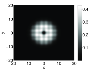
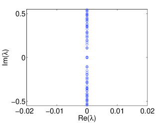
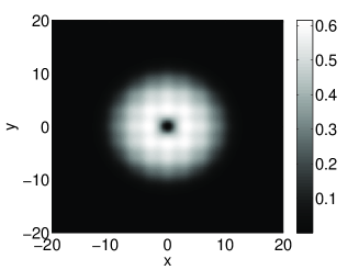
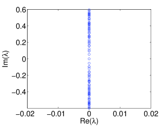
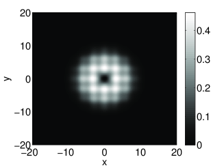
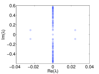
Figure 1: (Color Online) Top: profile (left) and spectrum (right) for a stable vortex with $\phi=0$ at $(V_{0},\mu)=(0.3,0.8)$. Middle: stable vortex with $\phi=\pi/2$ at the point $(0.1,0.8)$ in our parameter plane. Bottom: same for the unstable case at the intersection of the slices from the previous image, $(0.3,0.8)$.

On the other hand, when the vortex of single charge is located at a local minimum ($\phi=\pi/2$), instability sets in for a sufficiently modulated trap (i.e., for $V_{0}\approx 0.2$) and the solutions remain unstable essentially throughout their interval of existence. Notice that for each value of $\mu$, the solution can only sustain a certain level of modulation from the optical lattice, before it finally degenerates into the zero solution (beyond a certain critical, $\mu$-dependent OL strength). Typical examples of the subcritical and supercritical profiles and their corresponding spectra for the relevant $S=1$ mode are shown in Fig. 1. It is evident that in this case, beyond the critical $V_{0}$, a mode becomes unstable through an oscillatory instability associated with an eigenvalue quartet. Both the existence regime (top left panel) and the stability regimes (top right panel) of such waveforms are illustrated in Fig. 2 (the figure also contains relevant one-parameter cross-sections of the number of atoms and of the eigenvalue of the most unstable mode of the linearization).

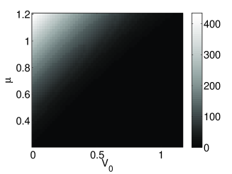
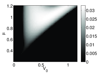
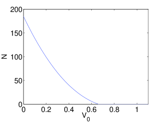
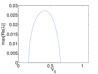
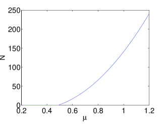
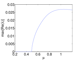
Figure 2: (Color Online) Top: the number of particles, $N$, is shown as a contour plot in the two-parameter plane of $(V_{0},\mu)$ in the left panel, while the maximum real part of $\lambda$ is shown in a similar way in the right panel for a single charged vortex with $\phi=\pi/2$. Middle: slices of $N(V_{0})$ (left) and ${\rm max}[{\rm Re}(\lambda(V_{0}))]$ (right) for $\mu=0.8$. Bottom: slices of $N(\mu)$ (left) and ${\rm max}[{\rm Re}(\lambda(\mu))]$ (right) for $V_{0}=0.3$.

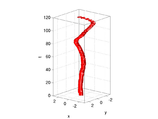
Figure 3: (Color Online) The dynamics of the unstable mode when $\phi=\pi/2$ for parameter values $(0.3,0.8)$. We show an isosurface of the vorticity, or curl of the velocity field ($\nabla\times\{\frac{-i}{|u|^{2}}[u^{*}\nabla u-u\nabla u^{*}]\}$) over time. This clearly illustrates the winding out of the vortex towards the periphery of the BEC cloud.

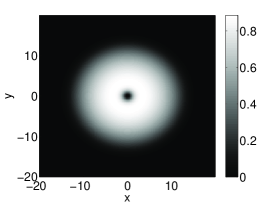
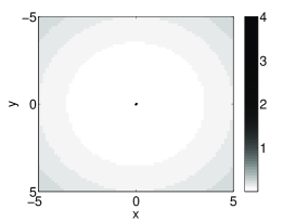
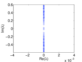
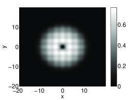
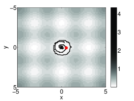
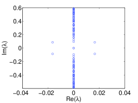
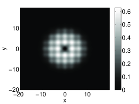
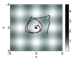
Figure 4: (Color Online) The vortex trajectory for 450 time units for some example charge 1 solutions are given above, center, with the respective stationary solutions, left, and spectra, right. All solutions are with $\mu=1$ and are overlayed on top of the external potential in order to clarify the setting. The top row is for $V_{0}=0$, middle is $V_{0}=0.2$, and the bottom row is for $V_{0}=0.4$. The red dot represents $\textbf{p}(t^{*})$ (see 4, 6). The value of $t^{*}$ is $300$ for the middle case and $134$ for the bottom.

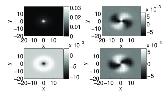
Figure 5: (Color Online). The real (top row) and imaginary (bottom row) parts of the linearization eigenvectors $W_{1}$ (left column) and $W_{2}^{*}$ (right column) corresponding to the unstable eigenvalue of the charge 1 solution with $\phi=\pi/2$ for parameter values $(V_{0},\mu)=(0.4,1)$ as in the evolution from the bottom row of Figure 4. Notice the majority of the support of $W_{1}$ is real valued and located at the vortex core. This accounts for the dominant feature of the dynamics of the perturbed solution, namely, the displacement from it’s original location. The apparent vorticity of the secondary mode, $W_{2}^{*}$, then contributes to the circular path.

Our stability calculations above are corroborated by direct numerical experiments involving the dynamical evolution of the vortices. We perturb the stationary state at unstable parameter values (for $\phi=\pi/2$) in the direction $\tilde{u}$ of its unstable eigenmode. We introduce the initial condition $u+\tilde{u}$ into our integrator, in this case a Runge-Kutta, fourth order scheme. Then, we integrate with the modest time step of $dt=10^{-2}$ afforded (stability-wise) by this method. The instability is clearly present and the vortex spirals out from the center of the condensate within the first 100 time units, as is shown in figure 3. We note in passing that this result is consonant with the earlier findings of pgk .

It is interesting enough to reiterate that for $\phi=\pi/2$, the instability growth rate is zero for small $V_{0}$, while for larger $V_{0}$, it becomes nonzero, in fact increasing initially as a function of $V_{0}$ as seen in Fig. 2 (before it eventually decreases back to zero along with the solution, for very strong lattices). This indicates that the vortices should spiral outward faster for larger $V_{0}$ (with the exception of the case of very strong lattices), which is perhaps counter-intuitive. In addition to the vorticity dynamics illustrated in figure 3, this fact is confirmed by observing the trajectory $\textbf{p}(t)$, defined below, of the initially stationary vortex slightly perturbed by a random noise of amplitude $\pm 0.05\%$ of the maximum amplitude of the solution, for different values of $V_{0}$ in the runs of Fig. 4. In these runs, the location of the vortex center is obtained by

$$\textbf{p}(t)=\frac{1}{||v||_{2}^{2}}(\int x|v|^{2}dA,\int y|v|^{2}dA),$$ (4)

where v(x,y,t) is the vorticity,

$$v(x,y,t)=\nabla\times\{-\frac{i}{|u|^{2}}[u^{*}\nabla u-u\nabla u^{*}]\}.$$ (5)

A related quantitative diagnostic is defined as

$$t^{*}={\rm min}\{t;||\textbf{p}(t)||_{2}>0.5\},$$ (6)

illustrating the time at which the vortex arrives at a distance of $0.5$ from its initial central location ($||\cdot||_{2}$ is the $L_{2}$ norm of Euclidean distance). In the absence of external potential, the perturbed vortex remains at the center of the harmonic trap for the entire simulation time of 450 units (see top row of Fig. 4). For a slightly larger value of $V_{0}=0.2$ it becomes slightly unstable due to a small magnitude eigenvalue quartet (with ${\rm max(Re}(\lambda))=0.0165$) which emerges. See the middle row of Fig. 4, and notice the (red) dot in the center image presenting the dynamics. This corresponds to $\textbf{p}(t^{*})$, where $t^{*}=300$, which represents the first time the vortex leaves the radius of $0.5$ from its original position. Notice that subsequently the perturbed vortex remains within the local minimum of the lattice for the duration of 450 time units. As $V_{0}$ is increased further to the value of $V_{0}=0.4$, depicted at the bottom row of the Fig. (4), it moves away from the initial location faster, having a critical time of $t^{*}=134$. This is in line with the fact that this case corresponds to a larger growth rate with ${\rm max(Re}(\lambda))=0.0307$. We should point out that this outward from the center motion of the vortex core may, in fact, be expected on the basis of the unstable eigenmodes of the linearization analysis shown in Fig. 5. There, it can be seen that the dominant instability eigenmode has a maximum (real) amplitude at the center and hence, when amplified, it will lead to the displacement of the vortex core from the center of the trap. The vorticity of the secondary mode will then contribute to the circular trajectory.

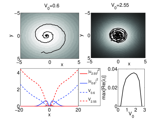
Figure 6: (Color Online) The above results are for the Gaussian dimple potential given in equation (7) with $\sigma=2\sqrt{10}$. The top row displays the (perturbed) vortex trajectory for $350$ time units of two solutions with fixed $\mu=0.99$. The left panel is for the value $V_{0}=0.6$, and the vortex is able to escape the confines of the dimple, while in the right panel, where $V_{0}=2.55$, the vortex remains in the deep dimple which has the approximate form of a harmonic potential itself, of frequency $2\sqrt{V_{0}}/\sigma$. The bottom left panel shows the potential (dotted) and the density proifile (solid) for $V_{0}=0.6$ (blue) and $V_{0}=2.55$ (red). The corresponding instability growth rate branch is given in the bottom right panel. It is interesting that, while the growth rates in the two cases are comparable, the parabolic nature of the deep dimple ($V_{0}=2.55$) prevents the spiraling out of the vortex during dynamical evolution.

It is interesting to compare these results with the work of prl_npp where the effect of sound emission and corresponding spiraling of the vortex away from the center of a magnetic trap with an additional radial dimple potential is considered. In the latter case, it was observed that for small amplitude of the dimple potential, the sound emission and vortex spiraling were facilitated, while for larger amplitudes of the dimple, the vortex was trapped within the dimple. While we point out that the case of prl_npp appears to have a reverse dependence of the evolution dynamics on the strength of the additional potential (to the magnetic one), we should also point out that there are fundamental differences between the two cases such as for instance the radial form of the dimple potential in comparison with the anisotropic spatial dependence of the periodic potential considered herein. In fact, we have performed stability computations in the context of the trap of prl_npp ,

$$V=V_{M}+V_{0}[1-\exp(\frac{2(x^{2}+y^{2})}{\sigma^{2}})].$$ (7)

We found a similar instability and dependence of its growth rate on $V_{0}$ (the strength of the dimple amplitude) as in our optical lattice results above (see the bottom right panel of Fig. 6); our numerical experiments on the evolution of the instability, on the other hand, confirm the findings of prl_npp (see the top row of Fig. 6).

III.2 $S=2$ Vortices

We now turn to the case of the doubly quantized vortex. Again, when $V_{0}=0$, we observe the solutions disappear at the linear QHO limit of $\mu=0.3$. Our results in the $V_{0}=0$ continuation over $\mu$ are consistent with those of pu . In particular, there are windows of stability along this branch for $\mu$ in the intervals $(0.45,0.75)$ and $(0.85,1)$. Then, as we fill out the surface of solutions in $V_{0}$ we observe in Fig. 7 a similar behavior of $N$ (as for the $S=1$ vortices), while the stability intervals appear to narrow as $V_{0}$ increases. Furthermore the stability landscapes appear to be quite similar for $\phi=0$ and $\phi=\pi/2$, as can be observed in the comparison of the upper right corners of figures 7 and 10. While the stability intervals quickly narrow as $V_{0}$ increases, it is worthwhile to note that stable solutions with a considerable amount of modulation by the optical lattice can still be identified.

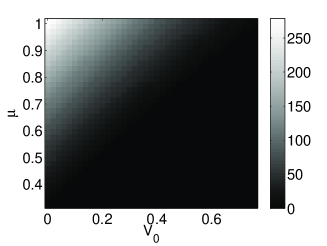
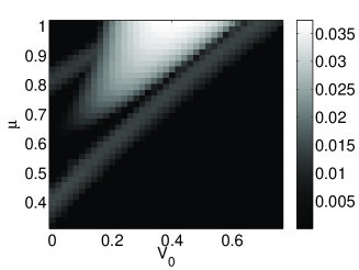
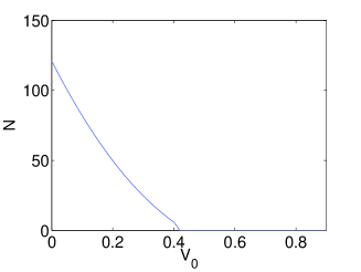
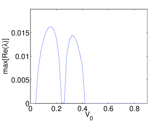
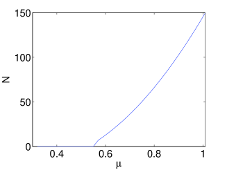
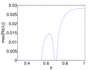
Figure 7: (Color Online) The corresponding images to Fig. 2 for a double charge vortex with $\phi=\pi/2$ in the same layout as for the single charge case in Fig. 2. $V_{0}$ slices are for $\mu=0.71$ and $\mu$ slices are for $V_{0}=0.24$.

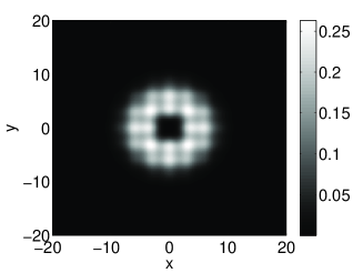
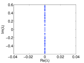
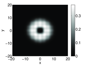
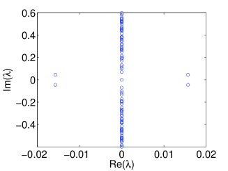
Figure 8: (Color Online) Stable (top, $(0.25,0.71)$) and unstable (bottom, $(0.13,0.71)$) double charge vortices (both their profiles and their corresponding spectral planes of eigenvalues) with $\phi=\pi/2$.

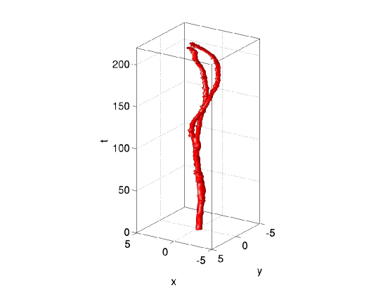
Figure 9: (Color Online) The space-time dynamics, similarly to Fig. 3, of the unstable mode when $\phi=\pi/2$ for parameter values $(0.13,0.71)$.

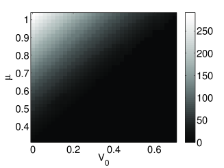
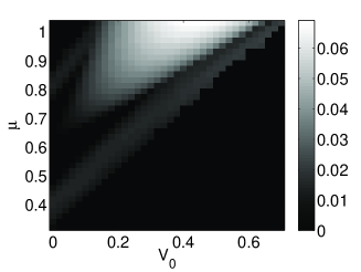
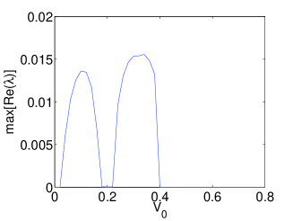
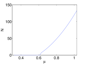
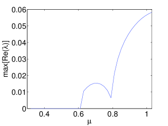
Figure 10: (Color Online) Same as figure 7 except with $\phi=0$. $V_{0}$ slices are for $\mu=0.71$ again and $\mu$ slices are for $V_{0}=0.3$.

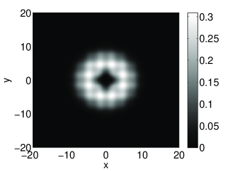
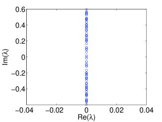
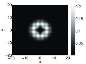
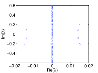
Figure 11: (Color Online) Similarly to Fig. 8, stable (top, $(0.21,0.71)$) and unstable (bottom, $(0.3,0.71)$) double charge vortices but now for $\phi=0$.

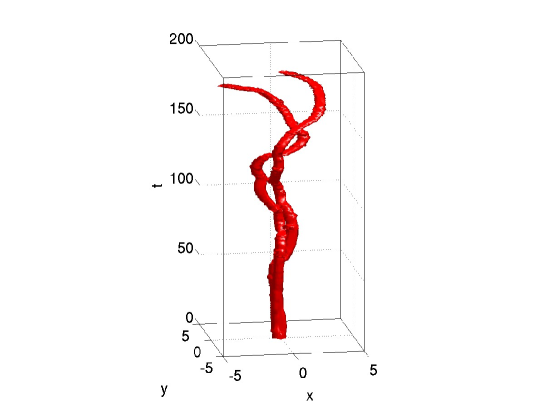
Figure 12: (Color Online) The space-time dynamics of the unstable mode when $\phi=0$ for parameter values $(0.3,0.71)$ is illustrated.

The dependence of the structure of the solutions on the phase of the OL, $\phi$, becomes apparent in the case of these higher charged vortices. In the case $\phi=\pi/2$, the vortex is centered at a local minimum of the lattice and therefore, when it merges with the neighboring local minima of the condensate background density, forms either an ’X’ or a square comprised of four local maxima of the lattice (minima of the condensate background), depending on the relative size of the condensate ($\mu$) and the lattice ($V_{0}$), as can be seen in figure 8. In the case of $\phi=0$, where the vortex merges with the neighboring local minima, it assumes the form of a cross comprised of five local maxima of the lattice, as is shown in Fig. 11.

Finally, we examine the dynamical evolution of vortices in the case of $\phi=\pi/2$ (Fig. 9) and $\phi=0$ (Fig. 12). Over time, both double charge vortices split into a pair of single charge vortices which follow one another around in an oscillatory spiral motion. Also, it is clear that the vortex located at the maximum (Fig. 11) has typically somewhat larger instability growth rates and in fact may possess two unstable eigenvalue quartets in its spectrum. This can also be observed to have a bearing in the evolution images, particularly as is highlighted in the contrast between figure 9, for parameter values for which the solution has a small instability growth rate, and figure 12, for parameter values for which the solution has a strong growth rate. The spiraling in Fig. 9 is slower and less violent than that of Fig. 12.

Dynamics were also performed for equal parameter values of $(0.25,0.8)$ and the vortex trajectory for 450 time units along with the profiles and spectra are presented in figure 13. The magnitude of the real part of the single quartet in each case is comparable, as are the corresponding dynamics. For $\phi=0$, ${\rm max[Re}(\lambda)]=0.036$, while for $\phi=\pi/2$, ${\rm max[Re}(\lambda)]=0.027$. While this slight discrepency is hard to detect from the trajectories shown in Fig. 13, we can define a similar diagnostic as in the single charge case. Here we define $\textbf{p}_{1}$ and $\textbf{p}_{2}$ as in equation 4 and $t^{**}={\rm min}\{t;{\rm max_{k}}(|{p}_{1}^{k}-p_{2}^{k}|)>1.5,k\in\{1,2\}\}$, where $\textbf{p}=(p^{1},p^{2})$, in order to investigate this fundamentally different type of instability. As we expect from the larger real part of its unstable quartet, $t^{**}=152$ when $\phi=0$ is smaller than $t^{**}=216$ when $\phi=\pi/2$.

It is interesting to remark here the apparent difference of this result with the case of the $S=1$ vortex, where the potential with $\phi=0$ induced stability, while that of $\phi=\pi/2$ could potentially lead to instability. However, an important clarification should be made here. The instability of the vortices with $S=1$ and that of the vortices with $S=2$ are fundamentally different. In particular, the former concerns the spiraling of the vortices away from the center of the trap (see Figs. 3 and 4). On the other hand, the latter predominantly involves the effect of splitting of the vortex of charge 2 into two vortices of charge $S=1$ (see Figs. 9, 12 and 13), As a result of this splitting, the two same charge vortices (as is discussed e.g. in us ), start rotating around each other (while, of course, spiraling away from the center of the trap). This type of effect (the break-up of the $S=2$ into two $S=1$ vortices) may even happen in the magnetic trap alone for solutions in one of the instability bands at $V_{0}=0$, rendering vortices of $S=2$ potentially unstable in that setting as discussed e.g. in pu .

In view of this, the two cases of $S=1$ and $S=2$ and their respective instability growth rates (and trends) should not be directly compared as they physically refer to different mechanisms. One of the two potentials (the $\phi=0$ case) can be thought of as a “local inhomogeneity” within the central well of the optical lattice, while the other one (the $\phi=\pi/2$) can be thought of, within the same region, as an approximate parabolic potential (modulated by an appropriately weak Gaussian past the first maximum of the optical lattice). While this picture can be fairly successful in capturing the stability characteristics of the optical lattice for small values of the chemical potential (results not shown), for strong nonlinearities (large chemical potentials) this picture is no longer valid. It is only in the latter strongly nonlinear regime where the growth rates of the instabilities in the cases of the two different phases of the optical lattice potential are substantially different. Hence it is a challenging task whether this difference can be intuitively understood, a question that is outside the scope of the present work. Interestingly, the unstable eigenmodes in this case have strong similarities in their spatial profile between the $\phi=0$ and $\phi=\pi/2$ cases and so only those for $\phi=\pi/2$ are shown in Fig. 14.

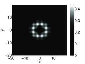
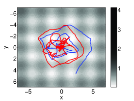
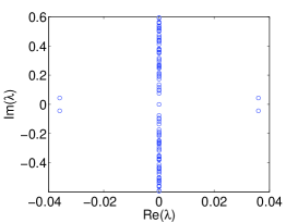
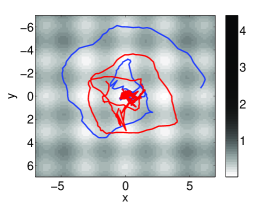
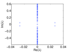
Figure 13: (Color Online) The top row contains the profile (left) spectrum (right) and temporal evolution for 450 time units of the charge 2 vortex with $\phi=0$, where one can visualize the splitting into tow charge 1 vortices in blue and red. The bottom row is the same for the case $\phi=\pi/2$. Parameter values are equal in both cases, $(0.25,0.8)$.

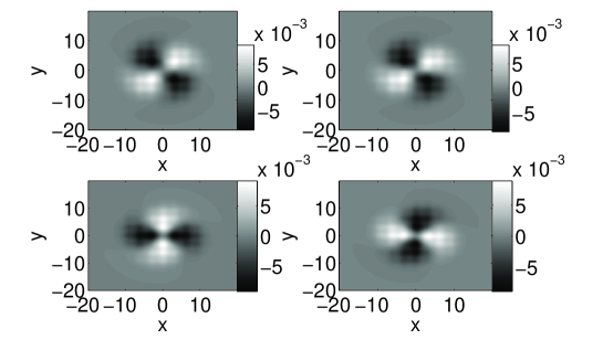
Figure 14: (Color Online). The same set of images as in 5 for the linearization around the charge 2 solution with $\phi=\pi/2$ for parameter values $(V_{0},\mu)=(0.25,0.8)$ as in the evolution from the bottom row of Figure 13. We note that for the case of $\phi=0$, the corresponding eigenmodes are qualitatively indiscernable from these shown here and are hence omitted.

IV $S=3$ Vortices

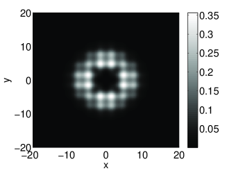
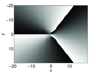
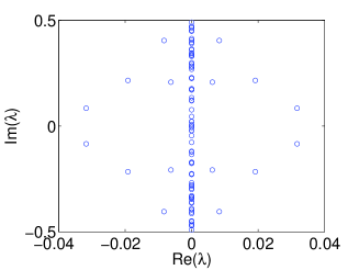
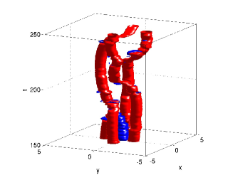
Figure 15: (Color Online) Top row: unstable charge $3$ vortex for $(0.44,1)$ for $\phi=0$; density profile (left) and corresponding phase diagram (right). Bottom row: spectrum of the solution (left) and dynamics of the unstable mode for parameter values $(0.44,1)$, where red is a positive isosurface and blue is a negative surface of equal magnitude.

Finally, we briefly touch upon the case of triple quantized vortices. In this setting, and depending on parameter values, we were able to identify two different fundamental types of solutions with this vorticity. One of them consists of four positively charged and one negatively charged vortex, forming a bound state with $S=3$, as is shown in Fig. 15. However, we were also able to identify settings where the entire structure appeared to be a single, point-like vortex as is shown in Fig. 16.

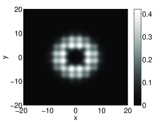
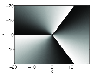
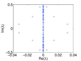
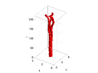
Figure 16: (Color Online) Top row: Unstable charge $3$ vortex for $(0.37,1)$ for $\phi=0$; density profile (left) and corresponding phase diagram (right). Bottom row: spectrum of the solution (left) and its dynamical evolution (right).

The dynamics over time of these solutions were consistent with the previous cases, as can also be seen in figures 15 and 16. The configuration with the $5$ single-charge vortices (of total $S=3$) exhibits an interesting type of instability development. Around $t=150$ the negative charge vortex in the middle collides with one of the $4$ positively charged vortices and they both dissappear, while the remaining $3$ $S=1$ structures begin to meander around the domain. On the other hand, the triple charge vortex in figure 16 splits into $3$ single charge vortices, which also spiral towards the periphery of the BEC cloud. All the cases shown for charge 3 are for $\phi=0$ , but we found similar results for $\phi=\pi/2$.

V Conclusion

In this work, we have examined in some detail the existence regime, stability regions and dynamical evolution of vortices of single, double and briefly also triple charge in a nonlinear Schrödinger equation involving both a parabolic and a periodic potential. This setting is particularly relevant to pancake-shaped BECs in the presence of magnetic trapping and optical lattices, but similar applications may arise in optics among other settings. We constructed two-parameter diagrams of the modes and their stability as a function of the solution’s chemical potential and the strength of the optical lattice. These continuations led to the insight that single-charged vortices are typically stable for cosinusoidal potentials, while they are typically unstable beyond a critical periodic potential strength for sinusoidal potentials. The instability is manifested through the outward spiraling of the vortex. In the case of $S=2$ vortices, the regions of instability widen (and, in fact, reach through all the way to the limit of no optical lattice, a feature that did not exist in the $S=1$ case) and now become fairly similar for the cosinusoidal and sinusoidal cases. The instability dynamics features the split up of the vortices and their subsequent rotation around each other, while they are both spiraling towards the outskirts of the BEC. Finally, both more complex scenaria of instability (involving many quartets of eigenvalues) and more complicated structures (including bound states of five vortices with total $S=3$) were found to arise in the $S=3$ case.

It would be of particular interest to examine the same type of solutions in the case of a three-dimensional magnetic and optical trapping. Adapting the numerical technology of Huepe , it should be possible to perform relevant three-dimensional existence and stability computations, by efficiently solving the linear system in the Newton method and identifying the dominant eigenvalues to infer how the stability is affected by introducing the $z$-dependence. In that problem, one can also use $\Omega$ as a parameter starting from the pancake-shaped limit of $\Omega\ll 1$, and going towards the spherical trap limit of $\Omega\rightarrow 1$. It would be especially interesting to observe how the stability properties are modified in the latter setting and how the unstable dynamics may develop. Such studies are currently in progress and will be reported in future publications.

References

- (1) A. S. Desyatnikov, Yu. S. Kivshar, and L. Torner, Prog. Optics 47, 291 (2005).
- (2) A.L. Fetter and A.A. Svidzinsky, J. Phys.: Cond. Matt. 13, R135 (2001).
- (3) P.G. Kevrekidis, R. Carretero-González, D.J. Frantzeskakis and I.G. Kevrekidis, Mod. Phys. Lett. B 18, 1481 (2005).
- (4) Pismen, Len M. Vortices in Nonlinear Fields., Oxford University Press (Oxford, 1999).
- (5) C. Sulem and P.L. Sulem, The Nonlinear Schrödinger Equation, Springer-Verlag (New York, 1999).
- (6) K.W. Madison, F. Chevy, W. Wohlleben and J. Dalibard, Phys. Rev. Lett. 84, 806 (2000).
- (7) M.R. Matthews, B.P. Anderson, P.C. Haljan, D. S. Hall, C.E. Wieman, and E. A. Cornell, Phys. Rev. Lett. 83, 2498 (1999).
- (8) J.R. Abo-Shaeer, C. Raman, J.M. Vogels, and W. Ketterle, Science 292, 476 (2001).
- (9) A.E. Leanhardt, A. Görlitz, A.P. Chikkatur, D. Kielpinski, Y. Shin, D.E. Pritchard and W. Ketterle, Phys. Rev. Lett. 89, 190403 (2002).
- (10) Y. Shin, M. Saba, M. Vengalattore, T.A. Pasquini, C. Sanner, A.E. Leanhardt, M. Prentiss, D.E. Pritchard and W. Ketterle, Phys. Rev. Lett. 93, 160406 (2004).
- (11) H. Pu, C. Law, J. Eberly and N. Bigelow, Phys. Rev. A 59, 1533 (1999).
- (12) Y. Kawaguchi and T. Ohmi, Phys. Rev. A 70, 043610 (2004).
- (13) M. Möttönen, T. Mizushima, T. Isoshima, M.M. Salomaa, K. Machida, Phys. Rev. A 68, 023611 (2003).
- (14) H. Saito and M. Ueda, Phys. Rev. A 69, 013604 (2004).
- (15) L.D. Carr and C.W. Clark, Phys. Rev. A 74, 043613 (2006).
- (16) H. Sakaguchi and B.A. Malomed, Europhys. Lett. 72, 698 (2005).
- (17) E.A. Ostrovskaya and Yu.S. Kivshar, Phys. Rev. Lett. 93, 160405 (2004).
- (18) E.A. Ostrovskaya, T.J. Alexander and Yu.S. Kivshar, Phys. Rev. A 74, 023605 (2006).
- (19) R. Kollár and R. Pego, Stability of vortices in two-dimensional Bose-Einstein Condensates: A mathematical approach, Preprint.
- (20) T. Kapitula, P.G. Kevrekidis and R. Carretero-González, Physica D 233, 112 (2007).
- (21) R.L. Pego and H.A. Warchall, J. Nonlin. Sci. 12, 347 (2002).
- (22) J.A.M. Huhtamäki, M. Möttönen and S.M.M. Virtanen, Phys. Rev. A 74, 063619 (2006).
- (23) E. Lundh and H.M. Nilsen, Phys. Rev. A 74, 063620 (2006).
- (24) P.G. Kevrekidis, R. Carretero-González, G. Theocharis, D.J. Frantzeskakis and B.A. Malomed, J. Phys. B 36, 3467 (2003).
- (25) A.B. Bhattacherjee, O. Morsch and E. Arimondo, J. Phys. B 37, 2355 (2004).
- (26) C.J. Pethick and H. Smith, Bose-Einstein condensation in dilute gases, Cambridge University Press (Cambridge, 2002).
- (27) L.P. Pitaevskii and S. Stringari, Bose-Einstein Condensation, Oxford University Press (Oxford, 2003).
- (28) Kelley, C.T. “Iterative Methods for Linear and Nonlinear Equations”, Frontiers in Applied Mathematics, Vol. 16. SIAM, Philadelphia, 1995.
- (29) N.G. Parker, N.P. Proukakis, C.F. Barenghi and C.S. Adams, Phys. Rev. Lett. 92, 160403 (2004).
- (30) T.P. Simula, S.M.M. Virtanen and M.M. Salomaa, Phys. Rev. A 65, 033614 (2002).
- (31) C. Huepe, L.S. Tuckerman, S. Metens, M.E. Brachet, Phys. Rev. A 68, 023609 (2003).