Diagrammatic approximations for the 2d quantum antiferromagnet: exact projection of auxiliary fermions

Abstract

We present diagrammatic approximations to the spin dynamics of the 2d Heisenberg antiferromagnet for all temperatures, employing an auxiliary-fermion representation. The projection onto the physical subspace is effected by introducing an imaginary-valued chemical potential as proposed by Popov and Fedotov. The method requires that the fermion number at any lattice site is strictly conserved. We compare results obtained within a self-consistent approximation using two different auxiliary-particle projection schemes, (1) exact and (2) on average. Significant differences between the two are found at higher temperatures, whereas in the limit of zero temperature (approaching the magnetically ordered ground state) identical results emerge from (1) and (2), providing the qualitatively correct dynamical scaling behavior. An interpretation of these findings is given. We also present in some detail the derivation of the approximation, which goes far beyond mean-field theory and is formulated in terms of complex-valued spectral functions of auxiliary fermions.

I Introduction and review

Auxiliary particles are a widely used tool in the theory of correlated electron systems. The principal difficulty in the treatment of these systems is the strong Coulomb repulsion $U$ for two electrons on the same localized orbital, usually of $d$ or $f$ character. In effective model Hamiltonians like the Heisenberg, $t$-$J$ , or Kondo model the large $U$ leads to a Gutzwiller projection onto the quantum-mechanical subspace, where none of the $d$- or $f$-orbitals may contain more than one electron at a time.

In this paper we will focus on the spin-1/2 quantum Heisenberg antiferromagnet in two spatial dimensions (2D) on a square latticeManousakis (1991),

$$H=\sum_{<i,j>}J\,\mathbf{S}_{i}\mathbf{S}_{j}\;\;,\;\;\;J>0$$ (1)

The sum covers all nearest-neighbor pairs $<i,j>$ . The model (1) may be obtained from the single-band Hubbard model for large $U$ with nearest-neighbor hopping amplitude $t$ (leading to $J=2t^{2}/U$) in the limit of a half-filled band with one electron per siteGros et al. (1987). It represents the simplest low-energy model for two-dimensional Mott insulators, in particular the CuO-planes in the undoped parent compounds for high-temperature superconductorsHayden et al. (1990); Keimer et al. (1992); Kim et al. (2001).

The restriction on states with no doubly occupied sites is reflected in the non-canonical commutation relations of spin operators,

$${}[\,S^{x}\,,S^{y}\,{}]=iS^{z}\neq\textrm{c-number}.$$ (2)

For an analytical approach to the model, Eq.(2) poses a severe difficulty, since the standard Wick’s theorem and many-body techniques cannot be appliedNegele and Orland (1988); Grewe and Keiter (1981); Bickers (1987); Izyumov and Skryabin (1988). A convenient way of circumventing this difficulty is to represent the spin operators in terms of canonical auxiliary-particle operators, of either fermionicAbrikosov (1965) or bosonicArovas and Auerbach (1988) character. The cost of this concept is the extension of the Hilbert space into unphysical sectors. These unphysical states have to be removed by imposing a constraint. In this work we use auxiliary fermions,

$$S^{\mu}_{i}=\frac{1}{2}\sum_{\alpha,\bar{\alpha}}f^{\dagger}_{i\alpha}(\sigma^{\mu})^{\alpha\bar{\alpha}}f_{i\bar{\alpha}}\;\;,\;\;\;Q_{i}=\sum_{\alpha}f^{\dagger}_{i\alpha}f_{i\alpha}=1\;\;,$$ (3)

$\sigma^{\mu}$ , $\mu=x,y,z$ are the Pauli matrices, and $\alpha=\uparrow,\downarrow$ is the fermion-spin index. Here and in the following we let $\hbar\equiv 1$ . The representation (3) fulfills the commutation relations (2) . The Fock space of the auxiliary fermions $f_{i\alpha}$ is spanned by the states

physical: $$|\uparrow\rangle=f^{\dagger}_{i\uparrow}|0\rangle\;\;,\;\;\;|\downarrow\rangle=f^{\dagger}_{i\downarrow}|0\rangle$$ (4a)

unphysical: $$|0\rangle\;\;,\;\;\;|2\rangle=f^{\dagger}_{i\uparrow}f^{\dagger}_{i\downarrow}|0\rangle$$ (4b)

where $|0\rangle$ denotes the vacuum, $f_{i\alpha}|0\rangle\equiv 0$ .

The projection onto the physical subspace can be performed in several waysBickers (1987), and for impurity models like the Kondo model or the single-impurity Anderson model the projection of auxiliary particles is a standard techniqueAbrikosov and Migdal (1970); Bickers et al. (1987). (For the latter model, auxiliary bosons have to be added to the schemeColeman (1984).) However, in lattice models like Eq.(1) the constraint $Q_{i}=1$ has to be enforced on each site $i$ independently. This leads to the so-called excluded-volume problemBrout (1961); Grewe and Keiter (1981) and prohibits an infinite-order resummation of the perturbation series in $J$ . In the limit of high spatial dimension the problem can be evaded within the (extended) dynamical mean-field theory. Here the infinite lattice system is approximately mapped onto a single siteKuramoto (1985); Metzner and Vollhardt (1989); Si and Smith (1996) or a small clusternot (a) coupled to a bath.

An alternative path starts from a mean-field-like treatment of the constraint, where the auxiliary charge $Q_{i}=1$ is fixed merely on the thermal averageNewns and Read (1987),

$$Q_{i}\to\langle Q_{i}\rangle=\langle Q_{1}\rangle=\sum_{\alpha}\langle f^{\dagger}_{1\alpha}f_{1\alpha}\rangle=1\;.$$ (5)

This condition is introduced into the Hamiltonian (1), (3) through a chemical potential $\mu^{f}$ for the auxiliary fermions. Due to the particle–hole symmetry of (1) we have $\mu^{f}=0$ . The approximation (5) is of great advantage, since now the perturbation theory in $J$ starts from non-interacting fermions, and we can make use of the standard Feynman-diagram techniques. Eq.(5) is also the starting point for numerous mean-field theories of correlated electron systems. An improvement of the mean-field-like constraint (5) in a perturbative fashion has frequently been made by generalizing $\mu^{f}$ to a fluctuating Lagrange multiplier (see, e.g., Ref. Bickers, 1987) .

The Popov–Fedotov approach: The method proposed by Popov and FedotovPopov and Fedotov (1988) enables one to enforce the auxiliary-particle constraint exactly within an analytical calculation for the infinite systemGros and Johnson (1990); Bouis and Kiselev (1999); Kiselev and Oppermann (2000); Dillenschneider and Richert (2006). The approach starts from a “grand-canonical ensemble”,

$$H\to H^{\textrm{ppv}}=H-i\frac{\pi}{2}T\sum_{i}Q_{i}\;\;,\;\;\;Q_{i}=\sum_{\alpha}f^{\dagger}_{i\alpha}f_{i\alpha}\;\;,\;\;\;$$ (6)

with a homogeneous, imaginary-valued chemical potential

$$\mu^{f}=i\frac{\pi}{2}k_{B}T\equiv i\frac{\pi}{2}T\;.$$ (7)

$H$ is the spin Hamiltonian (1), written in terms of the auxiliary-fermion operators (3) .

There are two main requirements for the Popov–Fedotov method to work: The first is the conservation of the auxiliary charge $Q_{i}$ on each lattice site,

$${}[\,Q_{i}\,,H\,{}]=0\;\;,\;\;\;i=1,2,\ldots,N_{L}\;\;,$$ (8)

where $N_{L}$ denotes the number of sites (i.e., spins) in the system (1) . Since also ${}[\,Q_{i}\,,Q_{j}\,{}]=0$ , the eigenstates of $H$ and $H^{\textrm{ppv}}$ in the Fock space of the fermions can be specified by some auxiliary-charge configuration

$$c_{Q}=(Q_{1},Q_{2},\ldots,Q_{N_{L}})\;\;,\;\;\;Q_{i}\in\{0,1,2\}\;.$$ (9)

Physical states belong to the subspace with the configuration

$$c_{Q}^{phys}=(1,1,\ldots,1)\;.$$ (10)

For a given configuration $c_{Q}$ the Hamiltonian (1) has a specific set of eigenstates with quantum numbers $n_{Q}$ and energies $E(c_{Q},n_{Q})$ , i.e., Schrödinger’s equation reads

$$H|c_{Q},n_{Q}\rangle=E(c_{Q},n_{Q})|c_{Q},n_{Q}\rangle\;.$$ (11)

Consider now the partition function $Z^{\textrm{ppv}}$ for the grand-canonical Hamiltonian (6),

$$Z^{\textrm{ppv}} = \textrm{Tr}^{f}{}[\,e^{-\beta H^{\textrm{ppv}}}\,{}]$$

$$= \sum_{c_{Q}}\sum_{n_{Q}}\langle c_{Q},n_{Q}|\,e^{-\beta H^{\textrm{ppv}}}\,|c_{Q},n_{Q}\rangle\;\;,$$

$\textrm{Tr}^{f}$ denotes the trace in the enlarged Hilbert space of the auxiliary fermions, and $\beta=1/k_{B}T\equiv 1/T$ . With Eqs.(11) and (6) it becomes

$$Z^{\textrm{ppv}} = \sum_{Q_{1},\ldots,Q_{N_{L}}=0}^{2}\;\sum_{n_{Q}}\cdot$$

$$\mbox{}\cdot\langle c_{Q},n_{Q}|\,e^{-\beta E(c_{Q},n_{Q})}\,e^{i\frac{\pi}{2}Q_{1}}\cdots e^{i\frac{\pi}{2}Q_{N_{L}}}\,|c_{Q},n_{Q}\rangle$$

In addition to the $Q_{i}$-conservation, the Popov–Fedotov method requires that the Hamiltonian and the operators appearing in physical (i.e., observable) correlation functions destruct the unphysical states $|0\rangle$ , $|2\rangle$ . In the present case, Hamiltonian and correlation functions are composites of spin operators, and we have, using Eqs.(3) and (4b),

$$S_{i}^{\mu}|0\rangle=0\;\;,\;\;\;S_{i}^{\mu}|2\rangle=0\;.$$ (13)

Consider an arbitrary site $l$ with an unphysical auxiliary charge $Q_{l}\neq 1$ . From Eq.(13) it follows

$$Q_{l}\neq 1\,:\quad\left.E(c_{Q},n_{Q})\right|_{Q_{l}=0}=\left.E(c_{Q},n_{Q})\right|_{Q_{l}=2}\;\;,$$ (14)

that is, the spin at site $l$ seems to be removed from the Hamiltonian for all states $|c_{Q},n_{Q}\rangle$ with $Q_{l}=0$ or $2$ . Accordingly, the contribution from $Q_{l}=0,2$ to $Z^{\textrm{ppv}}$ is proportional to

$$\sum_{Q_{l}=0,2}\,e^{i\frac{\pi}{2}Q_{l}}=(1+e^{i\pi})=0\;.$$ (15)

In that way, the unphysical contributions from all sites $l=1,\ldots,N_{L}$ cancel in the grand-canonical partition function, i.e., only the physical charge configuration $c_{Q}^{phys}$ , Eq.(10), survives in $Z^{\textrm{ppv}}$ :

$$Z^{\textrm{ppv}}=(i)^{N_{L}}\sum_{n}\langle n|\,e^{-\beta E_{n}}\,|n\rangle\;.$$

Here $|n\rangle$ and $E_{n}$ denote the eigenstates and -energies of the Hamiltonian (1) in the physical subspace,

$$\begin{array}[c]{c}\displaystyle|n\rangle=|c_{Q}^{phys},n_{Q}\rangle\;\;,\;\;\;E_{n}=E(c_{Q}^{phys},n_{Q})\;\;,\\[8.61108pt] \displaystyle H|n\rangle=E_{n}|n\rangle\;.\end{array}$$ (16)

Thus we end up with

$$Z^{\textrm{ppv}}=(i)^{N_{L}}\,Z\;\;,$$ (17)

i.e., up to a constant prefactor, the (canonical, physical) partition function $Z$ for the Heisenberg model (1) is given by $Z^{\textrm{ppv}}$ .

The above argument, originally presented by Popov and Fedotov in Ref. Popov and Fedotov, 1988 , is extended to Green’s functions in Appendix A . It is found that any correlation function of spin operators may be calculated from the grand-canonical Hamiltonian (6). In particular, the imaginary time-ordered spin susceptibility

$$\chi^{\mu\bar{\mu}}_{ij}(\tau-\tau^{\prime})=\frac{1}{Z}\mbox{Tr}{}[\,e^{-\beta H}\mathcal{T}_{\tau}\{S^{\mu}_{i}(\tau)S^{\bar{\mu}}_{j}(\tau^{\prime})\}\,{}]$$ (18)

can be obtained from

$$\chi^{\mu\bar{\mu}}_{ij}(\tau-\tau^{\prime})=\langle\mathcal{T}_{\tau}\{S^{\mu}_{i}(\tau)S^{\bar{\mu}}_{j}(\tau^{\prime})\}\rangle^{\textrm{ppv}}$$ (19)

with $\mu,\bar{\mu}\in\{x,y,z\}$ . The expectation value is calculated in the enlarged Fock space,

$$\langle\ldots\rangle^{\textrm{ppv}}=\frac{1}{Z^{\textrm{ppv}}}\textrm{Tr}^{f}{}[\,e^{-\beta H^{\textrm{ppv}}}\,\ldots\,{}]\;\;,$$ (20)

with $Z^{\textrm{ppv}}$ as defined in Eq.(I) above. The “modified Heisenberg” pictureNegele and Orland (1988) for spin operators reads

$$S^{\mu}_{i}(\tau)=e^{\tau H}S^{\mu}_{i}e^{-\tau H}=e^{\tau H^{\textrm{ppv}}}S^{\mu}_{i}e^{-\tau H^{\textrm{ppv}}}\;\;,$$ (21)

using again Eq.(13) . Similarly, the local magnetization is given by

$$\langle S^{\mu}_{i}\rangle=\frac{1}{Z}\textrm{Tr}{}[\,e^{-\beta H}S^{\mu}_{i}\,{}]=\langle S^{\mu}_{i}\rangle^{\textrm{ppv}}\;.$$ (22)

It should be emphasized that expectation values of unphysical operators are meaningless within the Popov–Fedotov scheme: E.g., the auxiliary-fermion charge $Q_{i}$ introduced in Eq.(3) does not destruct the unphysical states (4b), and one has

$$\langle Q_{i}\rangle\boldsymbol{\neq}\langle Q_{i}\rangle^{\textrm{ppv}}\;.$$ (23)

For the l.h.s. we know that $Q_{i}=1$ in the physical Hilbert space. For the r.h.s., however, we obtain $\langle Q_{i}\rangle^{\textrm{ppv}}=(1+i)$ . The calculation is given in Appendix A .

Average projection: For comparison, we also want to use the mean-field-like treatment of the auxiliary-fermion constraint mentioned below Eq.(5) . Since the (real-valued) chemical potential added to the Hamiltonian (1), (3) turns out to be zero, due to the particle–hole symmetry of (1), the calculation of a spin-correlation function or magnetization amounts to just enlarging the Hilbert space into the Fock space of the auxiliary fermions. The equivalents of the Eqs.(19), (22), and (23) then read

$$\chi^{\mu\bar{\mu}}_{ij}(\tau-\tau^{\prime})\simeq\langle\mathcal{T}_{\tau}\{S^{\mu}_{i}(\tau)S^{\bar{\mu}}_{j}(\tau^{\prime})\}\rangle^{\textrm{av}}$$ (24)

and

$$\langle S^{\mu}_{i}\rangle\simeq\langle S^{\mu}_{i}\rangle^{\textrm{av}}\;\;,$$ (25)

whereas

$$\langle Q_{i}\rangle=\langle Q_{i}\rangle^{\textrm{av}}=1$$ (26)

with

$$\langle\ldots\rangle^{\textrm{av}}=\frac{1}{Z^{\textrm{av}}}\textrm{Tr}^{f}{}[\,e^{-\beta H}\ldots\,{}]\;\;,\;\;\;Z^{\textrm{av}}=\textrm{Tr}^{f}{}[\,e^{-\beta H}\,{}]\;.$$ (27)

The $\simeq$ sign in (24), (25) stands for the error introduced by the uncontrolled fluctuations of the fermion occupation numbers $Q_{i}$ into unphysical states. These fluctuations are absent in the Popov–Fedotov scheme.

In the following sections, results from the exact and the averaged constraint will be obtained within the same diagrammatic approximations. The effect of the constraint on physical quantities like the dynamical structure factor and magnetic transition temperature is going to be studied. It will turn out that at sufficiently low temperature the results for averaged and exactly treated constraint become equal. In addition we will show in some detail how a self-consistent approximation that goes far beyond mean-field theory, can be worked out within the Popov–Fedotov approach.

II Effect of the constraint: simple approximations

In order to compare results for the Heisenberg model (1) from average projection, Eq.(5), and exact projection using the Popov–Fedotov scheme, Eq.(6), we consider a more general grand-canonical Hamiltonian of auxiliary fermions, $\widetilde{H}=H-\mu^{f}\sum_{i}Q_{i}$ . With the model Hamiltonian (1) written according to (3), it reads

$$\widetilde{H} = -\mu^{f}\sum_{i}f^{\dagger}_{i\alpha}f_{i\alpha}\;+\;$$

$$\mbox{}+\;\frac{1}{2}\sum_{i,j}J_{ij}\frac{1}{4}\boldsymbol{\sigma}^{\alpha\bar{\alpha}}\boldsymbol{\sigma}^{\beta\bar{\beta}}f^{\dagger}_{i\alpha}f^{\dagger}_{j\beta}f_{j\bar{\beta}}f_{i\bar{\alpha}}\;.$$

Sums over spin indices $\alpha,\bar{\alpha},\beta,\bar{\beta}$ are implied. The antiferromagnetic coupling $J_{ij}$ is nonzero and equal to $J>0$ , if $i,j$ are nearest neighbors. Depending on the projection method, the chemical potential $\mu^{f}$ takes the value

$$\begin{array}[c]{lcrcl}\textrm{average projection:}&&\mu^{f}&=&0\;\;,\\[4.30554pt] \textrm{exact projection:}&&\mu^{f}&=&\displaystyle i\frac{\pi}{2}T\;.\end{array}$$ (29)

In the case of exact projection, the Hamiltonian (II) is no longer Hermitian. Nevertheless, physical quantities like the dynamical structure factor for spin excitations or the magnetization will come out real-valued.

Eq.(II) represents a system of canonical fermions with a two-particle interaction $\sim J$ and may therefore be treated using standard Feynman-diagram techniquesNegele and Orland (1988). The bare fermion-Green’s function, written as a matrix in spin space, reads

$$\overline{G}^{0}_{ij}(i\omega)=\delta_{ij}\frac{1}{i\omega+\mu^{f}}\;\;,$$ (30)

where $\omega=(2n+1)\pi T$ , $n\in\mathbb{Z}$ is a fermionic Matsubara frequency. For the case of exact projection, $\mu^{f}=i\pi T/2$ , there is some common practicePopov and Fedotov (1988); Bouis and Kiselev (1999); Kiselev and Oppermann (2000) to absorb $\mu^{f}$ into $i\omega$ and to re-define $\omega$ accordingly. Here we do not follow this line, but keep $\omega$ as introduced above (i.e., fermionic).

Free spins ($J=0$): The simplest case is given by setting $J=0$ . Using Eq.(3), the susceptibility (18), to be calculated from Eq.(19) or (24), is then given by a simple bubble,

$$\chi_{ij}^{\mu\bar{\mu}}(i\nu) = -\frac{1}{4}T\sum_{i\omega}\textrm{Tr}^{\sigma}{}[\,\sigma^{\mu}\overline{G}^{0}_{ij}(i\omega+i\nu)\,\sigma^{\bar{\mu}}\,\overline{G}^{0}_{ji}(i\omega)\,{}]$$

$$= \delta_{i,j}\,\delta_{\mu,\bar{\mu}}\,\delta_{\nu,0}\,\chi^{0}$$

with, using Eq.(30),

$$\chi^{0}=\frac{1}{2T}f(-\mu^{f})f(\mu^{f})\;.$$

$\nu=2n\pi T$ is a bosonic Matsubara frequency, $\textrm{Tr}^{\sigma}$ denotes a trace in spin space, and $f(x)=1/(e^{x/T}+1)$ is the Fermi function. Depending on the constraint method, the result is

$$\begin{array}[c]{lclcl}\textrm{average:}&&\displaystyle f(0)=\frac{1}{2}&\;\Rightarrow&\displaystyle\chi^{0}=\frac{1}{8T}\;\;,\\[8.61108pt] \textrm{exact:}&&\displaystyle f(\pm i\frac{\pi}{2}T)=\frac{1}{1\pm i}&\;\Rightarrow&\displaystyle\chi^{0}=\frac{1}{4T}\;.\end{array}$$ (31)

Two observations are in order: The imaginary chemical potential cancels out in the physical quantity $\chi^{0}$ , and the result with and without use of the exact auxiliary-particle projection is qualitatively the same (Curie law). With merely average projection in effect ($\mu^{f}=0$), the spin moment $S(S+1)$ extracted from the Curie law $\chi^{0}(T)\propto S(S+1)/T$ is reduced by a factor of 2 compared to the exact result. This is due to fluctuations of the fermion charge $Q_{i}$ .

Mean-field approximation: The simplest approach to the interacting system $J>0$ is the Hartree approximation, i.e., magnetic mean-field theory. This approximation does locally conserve the auxiliary-fermion charge $Q_{i}$ . Dyson’s equation for the auxiliary fermion reads

$$\overline{G}_{i}(i\omega)={}[\,i\omega+\mu^{f}-\overline{\Sigma}_{i}(i\omega)\,{}]^{-1}\;\;,$$ (32)

and in Hartree approximation the self energy is independent of $i\omega$ and given by

$$\overline{\Sigma}_{i}=\sum_{j}J_{ij}\frac{1}{2}\boldsymbol{\sigma}\underbrace{\textrm{Tr}^{\sigma}{}[\,\frac{1}{2}\boldsymbol{\sigma}\sum_{i\bar{\omega}}\overline{G}_{j}(i\bar{\omega})e^{i\bar{\omega}0_{+}}\,{}]}_{\displaystyle=\langle\mathbf{S}_{j}\rangle}\;.$$ (33)

Here the mean magnetization $\langle\mathbf{S}_{j}\rangle$ on the site $j$ has been identified. For a square lattice with coordination number $z=4$ and only nearest-neighbor interaction $J>0$ we assume a Néel state on the two sublattices $A$, $B$ ,

$$\langle\mathbf{S}_{A}\rangle=-\langle\mathbf{S}_{B}\rangle=-\langle S^{z}_{B}\rangle\,\mathbf{e}_{z}\;.$$

The fermion Green’s function for any site on $A$ becomes

$$\overline{G}_{A}(i\omega)={}[\,i\omega+\mu^{f}+\sigma^{z}h\,{}]^{-1}\;\;,\;\;\;h=\frac{zJ}{2}\langle S^{z}_{A}\rangle\;,$$

which leads to the self-consistent equation

$$\langle S^{z}_{A}\rangle=\frac{1}{2}{}[\,f(-h-\mu^{f})-f(h-\mu^{f})\,{}]\;.$$ (34)

For average projection, with $\mu^{f}=0$ , we find

$$\textrm{average projection:}\quad\quad h=\frac{z}{4}J\,\tanh\big{(}\frac{h}{2T}\big{)}\;.$$ (35)

Within the Popov–Fedotov scheme, using $\mu^{f}=i\frac{\pi}{2}T$ , one has

$$\textrm{exact projection:}\quad\quad h=\frac{z}{4}J\,\tanh\big{(}\frac{h}{T}\big{)}\;,$$ (36)

where the following expression for the Fermi function has been utilized,

$$f(x-i\frac{\pi}{2}T)=f(2x)+\frac{i}{2\cosh(x/T)}\;\;,$$ (37)

for a real-valued $x$ . In the physical observable (34) the imaginary part again cancels. Both projection schemes lead to the same self-consistent equation for the effective magnetic (Weiss) field $h$ , except for a factor of 2 in the temperature. Accordingly the equations result in different Néel temperatures,

$$\begin{array}[c]{lcrcl}\textrm{average projection:}&&\displaystyle T_{N}&=&\displaystyle\frac{z}{8}J\;\;,\\[8.61108pt] \textrm{exact projection:}&&\displaystyle T_{N}&=&\displaystyle\frac{z}{4}J\;.\end{array}$$

However, at zero temperature both projection methods lead to the same result,

$$\textrm{average \emph{and} exact projection:}\quad\lim_{T\to 0}\langle S^{z}_{A}\rangle=\frac{1}{2}\;.$$ (38)

That is, the unphysical reduction of the spin moment observed for the free spin, is completely restored in the magnetically ordered ground state. Apparently, the unphysical charge fluctuations are suppressed at $T\to 0$ .

III Effect of the constraint: self-consistent theory

The purpose of this section is to demonstrate the application of the Popov–Fedotov scheme within a self-consistent approximation that goes far beyond mean field. To our knowledge, the Popov–Fedotov approach has at present been applied in mean-field-like calculations with perturbative correctionsPopov and Fedotov (1988); Bouis and Kiselev (1999); Kiselev and Oppermann (2000); Dillenschneider and Richert (2006), but a self-consistent re-summation of the diagram series has not been attempted.

When choosing an approximation scheme, it has to be kept in mind that the automatic cancellation of unphysical states requires the auxiliary-fermion charge $Q_{i}$ to be conserved (this has been discussed in Section I above). In particular, the local gauge symmetry of the Hamitonian (II) under $f_{i\alpha}\to e^{i\varphi_{i}}f_{i\alpha}$ must not be broken. Accordingly, approximations leading to finite expectation values like $\langle f^{\dagger}_{i\alpha}f_{j\alpha}\rangle\neq 0$ or $\langle f_{i\uparrow}f_{j\downarrow}\rangle\neq 0$ cannot be used, while it is safe to consider so-called $\Phi$-derivable approximationsLuttinger and Ward (1960); Baym (1962). Spontaneous breaking of physical symmetries (e.g., spin rotation, lattice translation) may be included, since the respective order parameters are gauge invariant. As a consequence of the local gauge symmetry, the fermion Green’s function is always local,

$$\overline{G}_{ij}(i\omega)=\delta_{i,j}\,\overline{G}_{i}(i\omega)\;.$$ (39)

Here we focus on the physics of the Heisenberg model (1) in strictly two spatial dimensions at finite temperature $T>0$ . This system has been studied extensively in the past using a variety of numerical and analytical methods, in particular in view of experiments on cuprate superconductors in the undoped limitnot (b). The Hartree approximation discussed in Section II above is, of course, not appropriate for the 2D system, although the Néel-ordered ground state at $T=0$ appears to be qualitatively correctManousakis (1991); Brinckmann and Wölfle (2004). At finite $T$ the theorem of Mermin and Wagner requires the magnetization $\langle\mathbf{S}_{i}\rangle=0$ to vanish. Therefore we seek an approximation, where the susceptibility $\chi$ is self-consistently coupled back onto itself. Such an approximation has originally been proposed for the Hubbard modelBickers et al. (1989), and is commonly referred to as FLEX .

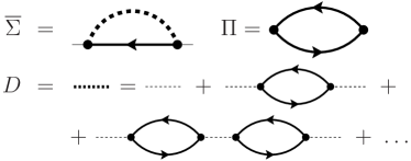
Figure 1: The self-consistent approximation (SCA) discussed in Section III , Eqs.(40) . Continuous lines denote the fermion Green’s function $\overline{G}$ , Eq.(39) , the thin dashed line represents $J$ , and dots are Pauli matrices $\times\,1/2$ .

For the Hamiltonian (II) with spin–spin interaction it takes the form shown in Fig. 1 . The fermion self-energy shown in the figure reads

$$\overline{\Sigma}_{i}(i\omega)=\frac{1}{4}T\sum_{i\nu}\sum_{\mu,\bar{\mu}}D_{ii}^{\mu\bar{\mu}}(i\nu)\,\sigma^{\mu}\,\overline{G}_{i}(i\omega+i\nu)\,\sigma^{\bar{\mu}}\;\;,$$ (40a)

$$\omega \nu \sigma^{\mu} \mu,\bar{\mu}=x,y,z i,j$$ and denote a fermionic and bosonic Matsubara frequency, respectively, a Pauli matrix,  . The renormalized spin–spin interaction on lattice sites is given by

$$D_{ij}^{\mu\bar{\mu}}(i\nu)=-J_{ij}\;+\;\sum_{l,k}J_{il}\,\chi_{lk}^{\mu\bar{\mu}}(i\nu)\,J_{kj}\;.$$ (40b)

The susceptibility $$\chi$$ represents the series of fermion-line bubbles in Fig. 1 ,

$$\chi_{ij}^{\mu\bar{\mu}}=\big{(}\Pi\,{}[\,1+J\Pi\,{}]^{-1}\big{)}_{ij}^{\mu\bar{\mu}}\;\;,$$ (40c)

with

$$\Pi_{i}^{\mu\bar{\mu}}(i\nu)=-T\sum_{i\omega}\frac{1}{4}\textrm{Tr}^{\sigma}{}[\,\sigma^{\mu}\,\overline{G}_{i}(i\omega+i\nu)\,\sigma^{\bar{\mu}}\,\overline{G}_{i}(i\omega)\,{}]\;.$$ (40d)

In the paramagnetic phase with lattice-translational symmetry we have

$$\overline{G}_{i}(i\omega)=\sigma^{0}\,G(i\omega)\;\;,\;\;\;\overline{\Sigma}_{i}(i\omega)=\sigma^{0}\,\Sigma(i\omega)\;\;,$$

and therefore

$$\Pi_{i}^{\mu\bar{\mu}}(i\nu)=\delta_{\mu,\bar{\mu}}\,\Pi(i\nu)\;.$$

The self-consistent equations (40) with Eq.(32) now turn into

$$\Pi(i\nu) = -\frac{T}{2}\sum_{i\omega}G(i\omega+i\nu)\,G(i\omega)\;\;,$$ (41a)

$$\chi(\mathbf{q},i\nu) = \frac{\Pi(i\nu)}{1+J(\mathbf{q})\Pi(i\nu)}\;\;,$$ (41b)

$$D(i\nu) = \frac{1}{N_{L}}\sum_{\mathbf{q}}J^{2}(\mathbf{q})\,\chi(\mathbf{q},i\nu)\;\;,$$ (41c)

$$\Sigma(i\omega) = \frac{3T}{4}\sum_{i\nu}D(i\nu)\,G(i\omega+i\nu)\;\;,$$ (41d)

$$G(i\omega) = \big{[}\,i\omega+\mu^{f}-\Sigma(i\omega)\,\big{]}^{-1}\;.$$ (41e)

The bare interaction in wave-vector space reads, for a square lattice in 2D with nearest-neighbor distance $$a\equiv 1$$ ,

$$J(\mathbf{q})=4J\,\gamma(\mathbf{q})\;\;,\;\;\;\gamma(\mathbf{q})=\frac{1}{2}{}[\,\cos(q_{x})+\cos(q_{y})\,{}]\;.$$ (41f)

Note that the bare $J$ in Eq.(40b) does not contribute to the local $D(i\nu)\equiv D_{ii}(i\nu)$ , Eq.(41c) , since $J_{ii}=0$ .

It has been emphasized above, that the fermion propagator and as a consequence the irreducible bubble are local, $G_{ij}=\delta_{i,j}\,G$ , $\Pi_{ij}=\delta_{i,j}\,\Pi$ . Nevertheless, the interesting measurablefoo quantity in the Eqs.(41) is the susceptibility $\chi(\mathbf{q})$ , which is wave-vector dependent through the bare interaction $J(\mathbf{q})$ , and therefore may describe even long-range fluctuations.

The SCA shown in Fig. 1 can be derived from a $\Phi$-functional in close analogyBickers et al. (1989) to the FLEX . Therefore, Eqs.(41) represent a conserving approximation and can be used with the averaged fermion constraint as well as the Popov–Fedotov approach. The case of average projection, $\mu^{f}=0$ , has been treated in detail in Ref. Brinckmann and Wölfle, 2004 . The magnetic correlation length $\xi(T)$ and the dynamical structure factor, derived from the susceptibility (41b) , came out quite satisfactorily when compared to known results, indicating that the diagrams in Fig. 1 indeed capture the important physics of the 2D system at low $T$ . In the following some of the results from Ref. Brinckmann and Wölfle, 2004 will be re-calculated using the Popov–Fedotov method, i.e., $\mu^{f}=i\frac{\pi}{2}T$ . It will turn out, that the imaginary-valued chemical potential requires the use of complex-valued spectral functions, leading to more involved equations than those derived in Ref. Brinckmann and Wölfle, 2004 for $\mu^{f}=0$ . The results calculated with both methods differ, except in the limit of vanishing temperature, where average and exact projection become equal, as will be presented below.

Equations for exact projection: Before discussing the numerical solution of Eqs.(41), we quote some important formal results derived in Appendix A . For a numerical implementation it is suitable to express all Green’s functions through their respective spectral functions. On account of the Hamitonian being non-Hermitian, the spectral function of the fermion Green’s function $G(i\omega)$ becomes complex-valued. $G$ is given by

$$(\overline{G}_{i})^{\alpha\bar{\alpha}}(i\omega)=\int_{0}^{1/T}\mathrm{d}\tau\,e^{i\omega\tau}\langle\mathcal{T}_{\tau}\{f_{i\alpha}(\tau)f^{\dagger}_{i\bar{\alpha}}(0)\}\rangle^{\widetilde{H}}\;\;,$$ (42)

with the thermal expectation value and $\tau$-dependence calculated in the enlarged fermion Fock-space with the Hamiltonian (II) . $G$ has the following spectral representation, $\displaystyle\overline{G}^{\alpha\bar{\alpha}}_{i}(i\omega)=\delta_{\alpha,\bar{\alpha}}G(i\omega)$ ,

$$G(i\omega)=\int_{-\infty}^{\infty}\mathrm{d}\varepsilon\,\frac{\widehat{G}(\varepsilon)}{i\omega+\mu^{f}-\varepsilon}\;\;,\;\;\;\mu^{f}=i\frac{\pi}{2}T\;.$$ (43)

The energy variable $\varepsilon$ is a real number. For simplicity a system invariant under lattice translations and spin rotations has been assumed. The spectral function $\widehat{G}$ is complex-valued,

$$\widehat{G}(\varepsilon)=\rho_{1}(\varepsilon)\;+\;i\rho_{2}(\varepsilon)\;.$$ (44)

In the Appendix A we also derive the sum rule

$$\int\mathrm{d}\varepsilon\,\widehat{G}(\varepsilon)=1\;\;,$$ (45)

$$\;\;\;\Rightarrow\;\;\;\int\mathrm{d}\varepsilon\,\rho_{1}(\varepsilon)=1\;\;,\;\;\;\int\mathrm{d}\varepsilon\,\rho_{2}(\varepsilon)=0\;\;,$$

$\varepsilon$ is again real valued. For the special case of spin degeneracy considered here, the fermion spectral-function in addition obeys the “particle–hole” symmetry,

$$\widehat{G}(-\varepsilon)=\widehat{G}(\varepsilon)^{\ast}\;\;,$$ (46)

$$\;\;\;\Rightarrow\;\;\;\rho_{1}(-\varepsilon)=\rho_{1}(\varepsilon)\;\;,\;\;\;\rho_{2}(-\varepsilon)=-\rho_{2}(\varepsilon)\;.$$

The relations (43), (44), (46) hold as well for the fermion self-energy $\Sigma$ .

For a numerical solution of the Eqs.(41), we introduce structure factors for $\Pi(i\nu)$ and $D(i\nu)$ according to

$$S^{0}(\omega)={}[\,1+g(\omega)\,{}]\,\Pi^{\prime\prime}(\omega)\;\;,\;\;\;\Pi^{\prime\prime}(\omega)=\textrm{Im}\,\Pi(\omega+i0_{+})\;\;,$$

$$U(\omega)={}[\,1+g(\omega)\,{}]\,\textrm{Im}\,D(\omega+i0_{+})\;\;,$$

with analytic continuation to the real axis via $\displaystyle\Pi(i\nu)\to\Pi(\omega+i0_{+})$ and $\displaystyle D(i\nu)\to D(\omega+i0_{+})$ , $\displaystyle\omega\in\mathbb{R}$ . The Bose function is denoted by $g(\omega)=1/(e^{\omega/T}-1)$ . As shown in detail in Appendix B , Eqs.(41) now turn into

$$U(\omega) = \int_{-\infty}^{\infty}\mathrm{d}\varepsilon\,\frac{S^{0}(\omega)\,\,\mathcal{N}(\varepsilon)\,\varepsilon^{2}}{{}\big{(}1+\varepsilon\,\Pi^{\prime}(\omega){}\big{)}^{2}+{}\big{(}\varepsilon\,\Pi^{\prime\prime}(\omega){}\big{)}^{2}}\;\;,$$ (47a)

$$\Pi^{\prime\prime}(\omega) = S^{0}(\omega)-S^{0}(-\omega)\;\;,$$ (47b)

$$\Pi^{\prime}(\omega) = \textrm{P}\!\!\int_{-\infty}^{\infty}\frac{\mathrm{d}\varepsilon}{\pi}\frac{\Pi^{\prime\prime}(\varepsilon)}{\varepsilon-\omega}\;\;,$$ (47c)

$$S^{0}(\omega) = \frac{\pi}{2}\int_{-\infty}^{\infty}\mathrm{d}\varepsilon\,\widehat{G}^{+}(\varepsilon)\,\widehat{G}^{-}(\varepsilon-\omega)\;\;,$$ (47d)

for the real (physical) functions $$U,S^{0},\Pi^{\prime\prime},\Pi^{\prime} \Pi^{\prime}$$ with the Kramers–Kroenig transform  , and

$$\widehat{G}^{+}(\omega) = {}[\,1-f(\omega-i\frac{\pi}{2}T)\,{}]\,\widehat{G}(\omega)\;\;,$$ (47e)

$$\widehat{G}^{-}(\omega) = f(\omega-i\frac{\pi}{2}T)\,\widehat{G}(\omega)\;\;,$$ (47f)

$$\widehat{G}(\omega) = \frac{\widehat{\Sigma}(\omega)}{{}\big{(}\omega-\overline{\Sigma}(\omega)\big{)}^{2}+{}\big{(}\pi\widehat{\Sigma}(\omega)\big{)}^{2}}\;\;,$$ (47g)

$$\widehat{\Sigma}(\omega) = \frac{3}{4\pi}\int_{-\infty}^{\infty}\mathrm{d}\varepsilon\,U(\varepsilon)\,\big{[}\,\widehat{G}^{+}(\omega-\varepsilon)+$$

$$\hskip 56.9055pt\mbox{}+\widehat{G}^{-}(\omega+\varepsilon)\,\big{]}\;\;,$$

$$\overline{\Sigma}(\omega) = \textrm{P}\!\!\int_{-\infty}^{\infty}\mathrm{d}\varepsilon\,\frac{\widehat{\Sigma}(\varepsilon)}{\omega-\varepsilon}\;\;,$$ (47i)

for the complex (unphysical) spectra $\widehat{G}^{\pm},\widehat{G},\widehat{\Sigma},\overline{\Sigma}$ with the Hilbert transform $\overline{\Sigma}$ . Note again that the energy arguments $\omega,\varepsilon$ are real-valued. As is also shown in the Appendix B , the Eqs.(47) can be somewhat simplified by utilizing the symmetry (46) . The imaginary chemical potential $i\frac{\pi}{2}T$ appears in Eq.(47e) and (47f), adding an imaginary part to the fermion spectra $\widehat{G}^{+}$ and $\widehat{G}^{-}$ via Eq.(37) .

The density-of-states that enters Eq.(47a) is defined as

$$\mathcal{N}(\varepsilon)=\frac{1}{N_{L}}\sum_{\mathbf{k}}\delta(\varepsilon-J(\mathbf{q}))\;\;,$$ (48)

and for the nearest-neighbor interaction (41f) in two dimensions it becomes

$$\mathcal{N}(\varepsilon)=\frac{K(m)}{2\pi^{2}J}\theta(4J-|\varepsilon|)\;\;,\;\;\;m=1-\left(\frac{\varepsilon}{4J}\right)^{2}\;\;,$$ (49)

with the complete elliptic integral of the first kind, $K(m)=\int_{0}^{1}\mathrm{d}t\,{}[\,(1-t^{2})(1-mt^{2})\,{}]^{-1/2}$ .

The physical output from the numerical iteration of Eqs.(47), (49) is the structure factor $U(\omega)$ of the effective interaction, which is essentially the local (on-site) spin-excitation spectrum, and the wave-vector dependent dynamical spin-structure factor

$$S(\mathbf{q},\omega)={}[\,1+g(\omega)\,{}]\,\textrm{Im}\left\{\frac{\Pi(\omega)}{1+J(\mathbf{q})\Pi(\omega)}\right\}\;\;,$$ (50)

with $\displaystyle\Pi=\Pi^{\prime}+i\Pi^{\prime\prime}$ . Furthermore, the magnetic correlation length $\xi(T)$ is extracted from the static magnetic susceptibility $\chi(\mathbf{q},0)$ : Eq.(41b), for $\mathbf{q}$ close to the Néel-ordering vector $\mathbf{Q}=(\pi,\pi)$ , i.e.,

$$J(\mathbf{q})\simeq-4J+(\mathbf{q}-\mathbf{Q})^{2}J\;\;,$$

leads to

$$\chi(\mathbf{q},0)=\frac{\Pi^{\prime}(0)}{1+J(\mathbf{q})\Pi^{\prime}(0)}\simeq\frac{1}{J}\frac{1}{\xi^{-2}+(\mathbf{q}-\mathbf{Q})^{2}}\;\;,$$

where $\Pi(0)=\Pi^{\prime}(0)$ has been used, and the correlation length is identified as

$$\xi(T)=\left(\frac{J\Pi^{\prime}(0)}{1-4J\Pi^{\prime}(0)}\right)^{1/2}\;.$$ (51)

For completeness, in Appendix C the self-consistent equations (47) are re-written in real-valued spectral functions. These Eqs.(93) can directly be compared to the Eqs.(A1) in Ref. Brinckmann and Wölfle, 2004 : Both sets of equations represent the same diagrammatic approximation shown in Fig. 1 , the former derived within the Popov–Fedotov scheme (exact projection), the latter within average projection.

IV Numerical results

The numerical results presented below are obtained from an iterative solution of the self-consistent equations (41), using the identical procedure and parameters for exact projection ($\mu^{f}=i\frac{\pi}{2}T$ , leading to Eqs.(93) in App. C) as well as average projection ($\mu^{f}=0$ , leading to Eqs.(A1) in Ref. Brinckmann and Wölfle, 2004). The procedure also utilizes Eqs.(49) and (51), which apply to both projection schemes. The data shown in Ref. Brinckmann and Wölfle, 2004 for the case of average projection have not been re-used in the present study.

Magnetic correlation length: The correlation length $\xi(T)$ is shown in Fig. 2 . $\xi(T)$ becomes larger than one lattice spacing for $T\lesssim J$ and reaches values up to $\simeq 1200$ lattice spacings for the lowest temperature $T=0.048J$ considered in this work. The numerical data shown in Fig. 2 are well reproduced by

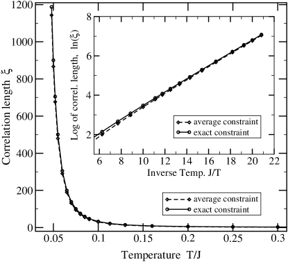
Figure 2: Main figure: Magnetic correlation length $\xi(T)$ from the numerical solution of the self-consistent approximation Fig.(1) for the 2D square lattice, in units of the lattice spacing. The continuous line with diamonds corresponds to Eqs.(47), where the Popov–Fedotov approach has been used. The dashed line with circles belongs to Eqs.(A1) in Ref. Brinckmann and Wölfle, 2004 , where the auxiliary-particle constraint has been approximated by its thermal average. Inset: The correlation length, plotted as $\ln(\xi)$ vs. $J/T$ . Shown is the temperature region $0.048\,J\leq T\leq 0.16\,J$ , where a fit to the data has been performed as described in the text.

$$\xi(T)=c\left(\frac{J}{T}\right)^{b}\exp\big{(}a\,\frac{J}{T}\big{)}\;.$$ (52)

The parameters $a,b,c$ are determined by plotting the data as $\ln(\xi)$ vs. $J/T$ (see the inset of Fig. 2) and a numerical fit of the function $\;\ln(c)+b\,\ln(J/T)+a\,J/T\;$ to the data. We find

$$\begin{array}[c]{lrcl}\textrm{average projection:}&a&=&0.296\\ &b&=&0.592\\ &c&=&0.393\\ \\ \textrm{exact projection:}&a&=&0.304\\ &b&=&0.418\\ &c&=&0.595\end{array}$$ (53)

At low temperatures the effect of the exact auxiliary-particle projection is only marginal, as is already apparent from inspecting Fig. 2 . The “spin stiffness” $a=2\pi\rho_{s}/J$ in the exponent in Eq.(52) is the same in both casesnot (c), $a\simeq 0.30$ , merely the power $b\simeq 0.5$ of the algebraic prefactor is slightly modified in going from average to exact projection.

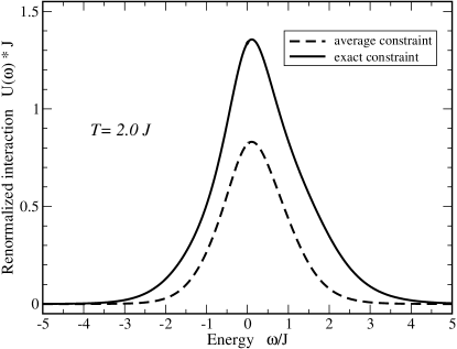
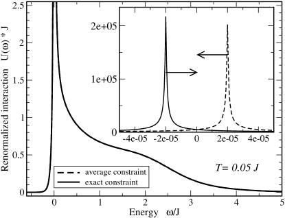
Figure 3: Top: The structure factor $U(\omega)$ , Eq.(47a), of the renormalized local interaction $D(i\nu)$ , Eq.(41c), at high temperature $T=2J$ . Dashed and continuous lines as in Fig. 2 . Bottom, main figure: $U(\omega)$ at low temperature $T=0.05J$ , corresponding to a correlation length $\xi\simeq 900$ . Bottom, inset: Same data as in the main figure, but zoomed around the energy $\omega=0$ . For clarity, the peaks for average constraint (dashed) and exact constraint (continuous) are shifted from their original position $\omega=0$ by 2e-05$J$ and -2e-05$J$ , respectively.

Spin spectral-function and energy scale: The almost vanishing effect of the auxiliary-particle constraint at low temperature is also visible in the spectra: Fig. 3 shows the effective interaction $U(\omega)$ , Eq.(47a), which is the structure factor of the $D(i\nu)$ given in Eq.(41c) . Since $J(\mathbf{q})^{2}$ in Eq.(41c) depends only weakly on $\mathbf{q}$ , $U(\omega)$ is essentally the local magnetic structure factor or spin-excitation spectrum. Note that Eq.(47a) is the same in the average-projected case, Eq.(A1h) in Ref. Brinckmann and Wölfle, 2004 . The data for low temperature, shown in the bottom panel of Fig. 3 , features a broad shoulder of width $\sim J$ , which is reminiscent of the box-like density-of-states for spin waves in 2D . Around zero energy $U(\omega)$ displays a huge peak (see the inset of the figure), which contains the critical fluctuations at $\mathbf{q}\simeq(\pi,\pi)$ close to the antiferromagnetic ordering wave-vector. The curves for average and exactly treated constraint are on top of each other; merely the amplitudes of the peaks at $\omega=0$ differ by a factor of $\mathcal{O}(1)$ . At high temperature $T=2J$ , on the contrary, the curves for average and exact constraint are well separated, in particular the total spectral weight is smaller for average projection. This can be seen from the data in the top panel of Fig. 3 . The reduction of spectral weight in $U(\omega)$ is related to an unphysical lack of local spin moment, which occurs if the constraint is not taken exactly. This will be discussed further below.

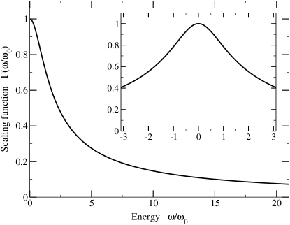
Figure 4: Main figure: The scaling function Eq.(58) of the renormalized spin–spin interaction, using the energy scale $\omega_{0}(T)$ from Eq.(57) and $\Gamma(0)\equiv 1$ . The curve shown here is the same for all temperatures $0.048\leq T/J\leq 0.13$ , corresponding to $1000\geq\xi(T)\geq 10$ , and independent of the auxiliary-particle constraint being treated exactly or on average. Inset: Detailed view of the region near $\omega=0$ .

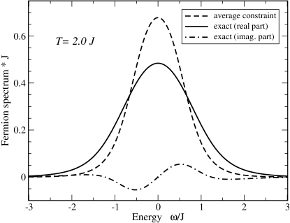
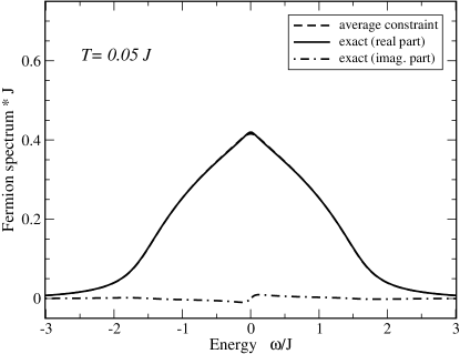
Figure 5: The spectral function $\widehat{G}(\omega)$ of the auxiliary fermion, introduced in Eqs.(42), (43) . For exact auxilary-fermion projection it is complex valued and given by Eq.(47g), for average projection Eq.(A1e) from Ref. Brinckmann and Wölfle, 2004 holds, with $\widehat{G}(\omega)$ being real. Top: high temperature, Bottom: low temperature. Parameters as in Fig. 3 .

The difference of peak amplitudes visible in the inset of Fig. 3 bottom can be traced back to the slightly different correlation length $\xi(T)$ , compare Eq.(53) . The influence of the absolute value of $\xi$ vanishes if the scaling behaviour of $U(\omega)$ is considered: We start from the dynamical scaling hypothesisChakravarty et al. (1989),

$$S(\mathbf{q},\omega)=\frac{1}{\omega_{0}}S^{st}(\mathbf{Q})\,\varphi(k\xi)\,\Phi(k\xi,\omega/\omega_{0})\;.$$ (54)

Here $S(\mathbf{q},\omega)$ is the dynamical structure factor Eq.(50), $S^{st}(\textbf{Q})$ denotes the static (equal-time) correlation function

$$S^{st}(\mathbf{q})=\langle S^{x}_{\mathbf{q}}S^{x}_{-\mathbf{q}}\rangle=\frac{1}{\pi}\int_{-\infty}^{\infty}\mathrm{d}\omega\,S(\mathbf{q},\omega)\;\;,\;\;\;$$ (55)

taken at the AF ordering wave vector $\mathbf{Q}=(\pi,\pi)$ . $\varphi(x)$ , $\Phi(x,y)$ are scaling functions, $\mathbf{k}=\mathbf{q}-\mathbf{Q}$ , and $\omega_{0}$ is the energy scale for critical fluctuations. At small energies $\omega\ll J$ we expect $U(\omega)\propto\int\mathrm{d}^{2}q\,S(\mathbf{q},\omega)$ , and from an intergration of Eq.(54) over wave-vector space there follows the scaling property

$$U(\omega)=\frac{1}{\omega_{0}}S^{st}(\mathbf{Q})\,\Gamma(\omega/\omega_{0})\;.$$ (56)

$\Gamma(y)$ is the (a priori unknown) scaling function for the local effective spin-spin interaction $U(\omega)$ . According to Eq.(54) the energy scale can be extracted from the numerical data, up to a constant prefactor, using

$$\omega_{0}=\left.\frac{S^{st}(\mathbf{Q})}{S(\mathbf{Q},\omega)}\right|_{\omega=0}\;.$$ (57)

We obtained the energy scale in the temperature range $0.048\leq T/J\leq 0.13$ , which corresponds to correlation lengths $1000\geq\xi\geq 10$ , using Eqs.(57), (55), and (50) . The scaling function is then determined for each temperature from Eq.(56),

$$\Gamma(\omega/\omega_{0})=\frac{U(\omega)}{U(0)}\;.$$ (58)

All curves $\Gamma(\omega/\omega_{0})$ , whether calculated with average or with exact auxiliary-particle constraint, agree to within numerical accuracy. The scaling function is shown in Fig. 4 . Deviations from scaling behaviour become visible only for higher energies $\omega/\omega_{0}>20$ . In particular, going from exact to average projection has no effect on the scaling behavior.

A slight difference in the low-temperature properties of the two auxiliary-particle methods shows up in the energy scale itself: From a linear regression on $\omega_{0}(T)\times\xi^{2}(T)$ , obtained from Eq.(57) and Eq.(51), we find

$$\begin{array}[c]{lrcl}\textrm{average:}&\omega_{0}\xi^{2}&=&(0.234\pm 0.002)\,J\;\;,\\ \textrm{exact:}&\omega_{0}\xi^{2}&=&(0.234\pm 0.002)\,J\;+\;0.089\,T\;.\end{array}$$ (59)

Nevertheless, the temperature behavior of the energy scale essentially is the same,

$$\omega_{0}(T)=0.23\cdot J\,(\xi)^{-2}\;\;,\;\;\;$$ (60)

which corresponds to a dynamical critical exponent $z=2$ .

Fermion propagator: Fig. 5 display the spectral function of the auxiliary-fermion propagator for the two projection methods. As has been discussed below Eq.(42), the spectrum $\widehat{G}(\omega)$ of the fermion is complex valued, if the auxiliary-particle constraint is enforced exactly via the imaginary-valued chemical potential $\mu^{f}=i\frac{\pi}{2}T$ . If the constraint is treated on the average using $\mu^{f}=0$ , $\widehat{G}(\omega)$ remains real. In Fig. 5 the spectrum $\widehat{G}(\omega)$ is shown for high (top panel) and low temperature (bottom). At high $T$ the spectra for exact and average constraint differ significantly, in particular the $\widehat{G}(\omega)$ from exact projection has a considerable imaginary part. At low temperature, on the other hand, the imaginary part is quite small, while the real part becomes equal to the spectrum of the average projection. In accordance with the results for spin-structure factor and correlation length, the projection onto the physical part of the fermion-Hilbert space has almost no effect at sufficiently low temperature.

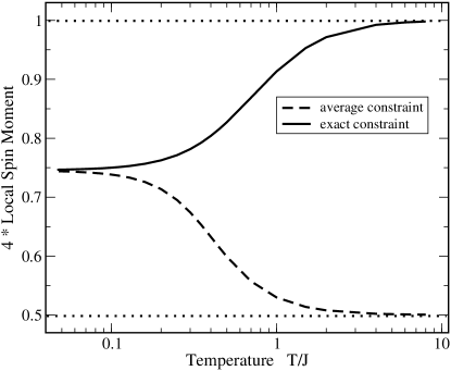
Figure 6: The local spin moment $S^{st}_{loc}$ as defined in Eq.(61), multiplied by 4 . The limiting values for $T\gg J$ given in Eq.(63) are indicated as dotted lines. The exact value, given by the sum rule (62), is $4\,S^{st}_{loc}=1$ .

Local spin moment: Another interesting quantity for studying the influence of the auxiliary-fermion constraint is the local spin moment, given by the local equal-time correlation function at an arbitrary site $i$ ,

$$S^{st}_{loc}=\langle S^{x}_{i}S^{x}_{i}\rangle=\frac{1}{N_{L}}\sum_{\mathbf{q}}S(\mathbf{q})\;.$$ (61)

The static structure factor $S(\mathbf{q})$ has been defined in Eq.(55) . For a spin-1/2 system in the paramagnetic phase $S^{st}_{loc}$ should fulfill the sum rule

$$S^{st}_{loc}=\frac{1}{3}(\mathbf{S}_{i})^{2}=\frac{1}{3}S(S+1)=\frac{1}{4}\;.$$ (62)

At very high temperature $T\gg J$ , interaction effects can be ignored, and $S^{st}_{loc}$ is given by the simple bubble $\Pi$ shown in Fig. 1 , calculated with free auxiliary fermions. With Eq.(41a) we have

$$T\gg J\,:\quad S^{st}_{loc} \simeq T\sum_{i\nu}\Pi(i\nu)\big{|}_{J=0}$$

$$= \frac{1}{2}\langle f^{\dagger}_{i\uparrow}f_{i\uparrow}\rangle^{\widetilde{H}}\,\langle f_{i\downarrow}f^{\dagger}_{i\downarrow}\rangle^{\widetilde{H}}\big{|}_{J=0}\;.$$

For both projection methods, the expectation values are to be taken in the generalized grand-canonical ensemble (II), (29) . For the case of average projection we find $\langle f^{\dagger}_{i\sigma}f_{i\sigma}\rangle=f(0)=1/2$ for any spin direction $\sigma=\pm 1$ , with exact projection we have $\langle f^{\dagger}_{i\sigma}f_{i\sigma}\rangle=f(-i\frac{\pi}{2}T)=\frac{1}{2}(1+i)$ . $f$ denotes the Fermi function. That is, for $T\gg J$ ,

$$\begin{array}[c]{lrcl}\textrm{average constraint:}&4\,S^{st}_{loc}&=&\frac{1}{2}\;\;,\\ \textrm{exact constraint:}&4\,S^{st}_{loc}&=&2\,\left|\frac{1}{2}(1+i)\right|^{2}=1\;.\end{array}$$ (63)

If the projection onto the physical Hilbert space is performed exactly, the sum rule (62) is correctly reproduced. With average projection, on the other hand, it is significantly violated. This is due to thermal charge fluctuations into unphysical, spinless states, which reduce the spin moment.

When temperature is lowered, we find a partly unexpected result: Fig. 6 shows $4\,S^{st}_{loc}$ from the numerical solution as function of $T$ . At high temperature the free-spin result is approached, whereas at low temperature the average and exact projection methods lead to the same value for $S^{st}_{loc}$ . This observation fits into the line of results obtained so far: at $T\to 0$ it does not matter whether the auxiliary-particle constraint is treated exactly or on the thermal average.

However, the local spin moment at $T\to 0$ , $4\,S^{st}_{loc}\simeq 0.75$ is too small. This is not due to an ill-treated constraint, but an artifact of the approximation to the interacting system. The local moment (61) measures the total spectral weight of spin excitations, averaged over the Brillouin zone. The self-consistent approximation we use, see Fig. 1 , apparently lacks some weight in the spin-excitation spectrum. In Ref. Brinckmann and Wölfle, 2004 we studied an approximation with a somewhat reduced self consistency (called “MSCA”), which delivered a better result for $S^{st}_{loc}$ at low $T$ , $4\,S^{st}_{loc}\simeq 0.85$ . Moreover, the wave-vector dependence of $S(\mathbf{q},\omega)$ came out better. However, the MSCA cannot straight-forwardly be extended to the Popov–Fedotov scheme, since we don’t know a $\Phi$-functional for that approximation to guarantee the conservation of the auxiliary-charge $Q_{i}$ , which is a necessary condition for the Popov–Fedotov method (see Section I above).

The limit $T\to 0$ : At first sight it seems trivial that the imaginary-valued chemical potential $\mu^{f}=i\frac{\pi}{2}T$ has almost no effect at $T\to 0$ : $\mu^{f}$ enters the self-consistent equations through the Fermi function $f(\omega-i\frac{\pi}{2}T)$ in Eqs.(47e) and (47f) . Assuming $T\ll\omega$ , Eq.(37) yields

$$T\ll\omega\,:\quad f(\omega-i\frac{\pi}{2}T)=\Theta(-\omega)+\mathcal{O}(e^{-2|\omega|/T})\;\;,$$ (64a)

which matches the case $$\mu^{f}=0 T=0 \omega_{0} T$$ (average projection) at  . On the other hand, the energy scale of spin excitations, Eq.(60), is exponentially small compared to  , therefore the opposite limit should apply,

$$T\gg\omega\,:\quad f(\omega-i\frac{\pi}{2}T)=\frac{1}{2}(1+i)+\mathcal{O}(\frac{\omega}{T})\;\;,$$ (64b)

adding a significant imaginary part to the fermion spectral-function $\widehat{G}(\omega)$ . It requires a solution of the set of Eqs.(47), however, to reveal that $\widehat{G}(\omega)$ has no featuresnot (d) at $\omega\lesssim\omega_{0}$ (see Fig. 5). The fermion spectrum is governed by its bandwidth $\sim J$ , and therefore the crossover from high-temperatures corresponding to Eq.(64b) to low temperatures, where Eq.(64a) becomes valid, happens at $T\sim J$ . A more physical interpretation is provided in the following Sections V and VI .

V Measuring the constraint

In order to understand the weak influence of the fermion constraint at low temperature, it is useful to calculate the auxiliary-charge fluctuations in average projection. Starting from Eq.(27), we have to calculate

$$\langle\Delta Q_{i}\,\Delta Q_{j}\rangle^{\textrm{av}}=\langle Q_{i}Q_{j}\rangle^{\textrm{av}}-\langle Q_{i}\rangle^{\textrm{av}}\,\langle Q_{j}\rangle^{\textrm{av}}\;.$$ (65)

Since all charges $Q_{i}$ are conserved, ${}[\,Q_{i}\,,\,H\,{}]=0$ , ${}[\,Q_{i}\,,\,Q_{j}\,{}]=0$ , the correlation function (65) may be obtained from the charge propagator in Matsubara space as

$$\chi^{Q}_{ij}(i\nu) = \int_{0}^{1/T}\mathrm{d}\tau\,e^{i\nu\tau}\langle\mathcal{T}_{\tau}\{\Delta Q_{i}(\tau)\,\Delta Q_{j}(0)\}\rangle^{\textrm{av}}$$ (66)

$$= \frac{1}{T}\,\delta_{\nu,0}\,\langle\Delta Q_{i}\,\Delta Q_{j}\rangle^{\textrm{av}}\;.$$

$\chi^{Q}_{ij}(i\nu)$ is conveniently calculated with the Feynman-diagram rules introduced in Sect. II , using the Hamiltonain (II) with $\mu^{f}=0$ and the bare fermion Green’s function (30) .

Free spins: In Section II we first discussed the limit $J=0$ . In that case, $\chi^{Q}$ is given by a simple bubble of bare fermion Green’s functions,

$$\chi^{Q}_{ij}(i\nu) = -T\sum_{i\omega}\textrm{Tr}^{\sigma}{}[\,\overline{G}^{0}_{ij}(i\nu+i\omega)\,\overline{G}^{0}_{ji}(i\omega)\,{}]$$

$$= \frac{1}{2T}\delta_{i,j}\delta_{\nu,0}\;\;,$$

that is,

$$J=0\,:\quad\langle\Delta Q_{i}\,\Delta Q_{j}\rangle^{\textrm{av}}=\delta_{i,j}\frac{1}{2}\;.$$ (67)

As expected, the auxiliary-charge fluctuations are finite. Note that $\chi^{Q}_{ij}(i\nu)$ is local ($\sim\delta_{i,j}$) and static, ($\sim\delta_{\nu,0}$) in accordance with Eq.(66), i.e., the conservation of the $Q_{i}$ .

Mean-field theory: The second example presented in Section II is the Hartree approximation. $\chi^{Q}$ is again given by the simple bubblenot (e), with $\overline{G}_{ij}^{0}$ replaced by

$$\overline{G}_{ij}(i\omega)=\delta_{i,j}{}[\,i\omega+(-1)^{i}\sigma^{z}\,h\,{}]^{-1}\;\;,$$

with the Weiss field $h$ given in Eq.(34) . For $T\ll J$ we obtain

$$\textrm{Hartree:}\quad\langle\Delta Q_{i}\,\Delta Q_{j}\rangle^{\textrm{av}}=\delta_{i,j}2\exp(-h/T)\;\;,$$ (68)

with $h=\frac{zJ}{4}+\mathcal{O}(e^{-J/T})$ . That is, in the magnetically ordered phase the unphysical charge fluctuations are strongly suppressed, since the fermions develop a charge gap similar to a spin-density-wave state.

Self-consistent theory: The approximation discussed in Sections III and IV requires a more elaborate calculation. For the case of average constraint, $\mu^{f}=0$ , the approximation given by Eqs.(41) and Fig. 1 has been studied earlier in Ref. Brinckmann and Wölfle, 2004 . In Section IV C of that paper the conserving-approximation scheme has been applied to the spin susceptibility, leading to a vertex function in the fermion bubble, which is determined by a Bethe–Salpeter equation. The corresponding diagrams are shown in Fig. 6 of Ref. Brinckmann and Wölfle, 2004 . For the auxiliary-fermion-charge susceptibility we want to calculate, the diagrams are exactly the same, except that the two spin vertices appearing in the bubble $\widehat{\Pi}$ in Fig. 6 are to be replaced by charge vertices $\sigma^{0}=1$ . The response function (66) then reads in wave-vector space

$$\chi^{Q}(\mathbf{q},0)=-T\sum_{i\omega}\textrm{Tr}^{\sigma}{}[\,\sigma^{0}\,\overline{G}(i\omega)\,\overline{\Gamma}(\mathbf{q},i\omega)\,\overline{G}(i\omega)\,{}]\;.$$

For $\langle\Delta Q\,\Delta Q\rangle^{\textrm{av}}$ merely the static limit $\displaystyle\lim_{\nu\to 0}\chi^{Q}(\mathbf{q},i\nu)$ is needed. With spin-rotation symmetry one has $\overline{G}=\sigma^{0}\,G$ , and it turns out that $\overline{\Gamma}=\sigma^{0}\,\Gamma$ (i.e., the charge and spin channels do not mix in the vertex function), leading to

$$\chi^{Q}(\mathbf{q},0)=-2T\sum_{i\omega}G(i\omega)^{2}\,\Gamma(\mathbf{q},i\omega)\;.$$ (69)

The vertex function is specified through the following Bethe–Salpeter equation, taken from the diagrams in Fig. 6 of Ref. Brinckmann and Wölfle, 2004 ,

$$\begin{array}[c]{l}\displaystyle\Gamma(\mathbf{q},i\omega)=1+\\[4.30554pt] \displaystyle\mbox{}+\frac{3}{4}T\sum_{i\omega_{1}}G(i\omega_{1})^{2}\,D(i\omega-i\omega_{1})\,\Gamma(\mathbf{q},i\omega_{1})-\\[12.91663pt] \displaystyle\mbox{}-\frac{3}{8}T\sum_{i\nu}G(i\omega+i\nu)\frac{1}{N_{L}}\sum_{\mathbf{k}}D(\mathbf{k}+\mathbf{q},i\nu)\,D(\mathbf{k},i\nu)\times\\[12.91663pt] \displaystyle\mbox{}\times T\sum_{i\omega_{1}}G(i\omega_{1})^{2}\,{}[\,G(i\omega_{1}+i\nu)+G(i\omega_{1}-i\nu)\,{}]\,\Gamma(\mathbf{q},i\omega_{1})\end{array}$$ (70)

The fermion Green’s function $G(i\omega)$ and the local spin-spin interaction $D(i\nu)$ have to be taken from the solution of the Eqs.(41) for $\mu^{f}=0$ . The non-local spin interaction appearing in (70) reads

$$D(\mathbf{q},i\nu)=-J(\mathbf{q})+J(\mathbf{q})^{2}\,\chi(\mathbf{q},i\nu)\;\;,$$

with $\chi$ from Eq.(41b) .

In Appendix D it is shown that the 2nd term in Eq.(70) actually becomes zero by symmetry arguments, i.e., the Bethe–Salpeter equation simplifies to

$$\Gamma(\mathbf{q},i\omega)=1+\frac{3}{4}T\sum_{i\omega_{1}}G(i\omega_{1})^{2}\,D(i\omega-i\omega_{1})\,\Gamma(\mathbf{q},i\omega_{1})$$ (71)

Instead of solving the last equation numerically, we find it more instructive to aim at an approximate analytical solution. We employ the static approximation introduced in Ref. Brinckmann and Wölfle, 2004 , i.e., let $D(i\nu)=D(0)\delta_{\nu,0}$ in Eq.(71) as well as the fermion self-energy (41d) . The calculation closely follows Sections IV A and C of Ref. Brinckmann and Wölfle, 2004 , leading to

$$\Gamma(\mathbf{q},i\omega)=\frac{1}{1-(\omega_{f}/2)^{2}G(i\omega)^{2}}\;\;,\;\;\;\omega_{f}=J\frac{16}{3\pi}+\mathcal{O}(T^{2})$$

for temperatures $T\ll J$ . $\omega_{f}$ is a typical 1/2 bandwidth of the continuous fermion spectrum, compare the bottom panel of Fig. 5 . Performing the Matsubara-sum in Eq.(69) eventually leads to

$$\chi^{Q}(\mathbf{q},0)=\frac{1}{\omega_{f}}\Phi^{Q}(T/J)\;\;,\;\;\;\Phi^{Q}(t)=\frac{4}{\pi}+\mathcal{O}(t^{2})\;.$$

If the vertex function is ignored, $\Gamma\to 1$ , the result does not change significantly, $\Phi^{Q}(t)\to\frac{16}{3\pi}+\mathcal{O}(t^{2})$ . Note that $\chi^{Q}$ is independent of $\mathbf{q}$ , i.e., local.

From Eq.(66) we thus find the auxiliary-charge fluctuations of our self-consistent approximation in average projection,

$$\textrm{self cons.:}\quad\langle\Delta Q_{i}\,\Delta Q_{j}\rangle^{\textrm{av}}=\delta_{i,j}\frac{3T}{4J}+\mathcal{O}(T^{3})\;.$$ (72)

Since the fermion spectrum is gaplessnot (d) around $\omega=0$ (see Fig. 5), and the vertex function has very little effect, $\chi^{Q}$ comes out Pauli-like. The explicit $T$ factor in Eq.(66) suppresses the charge fluctuations at low temperature. Compared to the magnetically ordered state described in mean-field (Hartree) theory, where the fermions develop a gap $\sim J$ (see Eq.(68)), the suppression of charge fluctuations is much weakernot (f). However, at $T\to 0$ the unphysical fluctuations still vanish, and the average projection becomes exact.

VI Summary and conclusions

Resummed perturbation theory is a powerful tool for calculating dynamical properties of strongly correlated electron systems. In this paper we focused on the spin-1/2 antiferromagnetic quantum Heisenberg model on the two dimensional square lattice. Summing infinite classes of contributions in perturbation theory is most economically done within a quantum-field-theoretic formulation employing canonical fields. We therefore use an auxiliary-particle representation of spin operators, which is a faithful representation in the physical sector of the Hilbert space.

The use of auxiliary fermions requires a projection onto the physical part of the fermion-Fock space, where the fermion charge $Q_{i}$ equals one for each lattice site.

While for a single lattice site the projection may be done exactly, e.g., by introducing an auxiliary-fermion energy $\lambda$ , which is sent to infinity at the end of the calculationAbrikosov (1965); Coleman (1984), these standard methods cannot directly be generalized to effect the projection at each lattice site independently (this would require handling a large number of independent limiting procedures, an impossible task in practice).

For lattice systems the most simple approach to the projection is an approximative treatment, where a global chemical potential (Lagrange multiplier) $\mu^{f}$ is introduced, which is sufficient to fulfill the constraint on the thermal average, $\langle Q_{i}\rangle=1$ .

However, Popov and Fedotov have proposed a rather unusual projection method, where a global imaginary-valued chemical potential $\mu^{f}=i\frac{\pi}{2}T$ leads to an exact cancellation of unphysical states, therefore enforcing the operator constraint $Q_{i}=1$ . Unfortunately, the Popov-Fedotov method may not straight-forwardly be generalized to systems away from particle-hole symmetryGros and Johnson (1990).

In this paper we explored the usability of this concept by identifying the conditions to be satisfied by any, necessarily self-consistent, approximation scheme. Most important is the conservation of the fermion charge $Q_{i}$ by the model Hamiltonian, ${}[Q_{i},H{}]=0$ . If the approximation under consideration violates this conservation law, results become meaningless (see Sec. I and App. A) . Therefore, self-consistent approximations are most safely based on the conserving-approximation principle. Any hopping of auxiliary fermions, for example, is precluded by this requirement: The fermions are strictly local entities. The physically observable momentum dependence of spin correlation functions originates from the momentum dependence of the exchange interaction.

Within the Popov–Fedotov approach the well known Feynman-skeleton-diagram expansion is applicable in conjunction with an exact projection of the auxilary particles onto the physical Hilbert space. We have shown in some detail how a self-consistent approximation, which goes far beyond mean-field theory similar to the “fluctuation-exchange approximation”, can be formulated using complex-valued spectral functions of the (unphysical) renormalized fermion propagator. The resulting equations have been solved by numerical iteration.

We applied the Popov-Fedotov method on several approximation levels: the free spin, the Hartree approximation (magnetic mean-field theory), and the above-mentioned self-consistent approximation, using both average projection ($\mu^{f}=0$) and exact projection ($\mu^{f}=i\frac{\pi}{2}T$) . The results obtained for the latter approximation show the expected suppression of the ordered state down to zero temperature, the exponential divergence of the spin correlation length, and a spin-structure factor consistent to the dynamical scaling hypothesis.

A comparison of the results from average and exact projection reveals that there is a significant effect of the exact projection at higher temperatures. In the limit of low temperature, however, the deviation of the average-constraint results from the exact-constraint results become (numerically) indistinguishable, except for the case $J=0$ (free spins).

In order to support this observation, we calculated the fluctuations $\langle\Delta Q_{i}\,\Delta Q_{j}\rangle$ of the auxiliary-fermion charge within the average-projection scheme. We find (by analytical calculation) $\;\lim_{T\to 0}\langle\Delta Q_{i}\,\Delta Q_{j}\rangle=0$ , except for the case of free spins, where $\langle\Delta Q_{i}\,\Delta Q_{j}\rangle$ stays finite as $T\to 0$ . That is, as long as the spin–spin interaction $J$ is taken into account, the fermion-charge fluctuations into unphysical Hilbert-space states are quenched at $T=0$ . If temperature is increased from zero, we find that $\langle\Delta Q_{i}\,\Delta Q_{j}\rangle$ raises continuously with $T$ .

These at first sight surprising results find their explanation in the tendency towards antiferromagnetic order in the interacting system, which helps to suppress the fluctuations in the fermion-occupation number: Starting from the physical (“true”) ground state, which features long-range magnetic orderManousakis (1991), a fluctuation of the fermion charge $Q_{l}=1$ at some site $l$ into an unphysical statenot (g) with $Q_{l}=0$ or $Q_{l}=2$ is equivalent to removing the spin $\mathbf{S}_{l}$ in the Hamiltonian (recall Eqs.(13) and (14)) . The lowest-lying state in this unphysical subspace thus lacks the binding energy of the spin at site $l$ , which is of order $J$ . Therefore, the ground state in the Fock space of arbitrary fermion occupancy is the “true” ground state in the physical segment, and the lowest-lying unphysical state is separated from the ground state by a gapnot (h) $\Delta E_{Q}\sim J$ .

Consequently, at low temperatures $T\ll\Delta E_{Q}$ , to a good approximation the exact projection may be omitted in favour of the technically somewhat simpler average-projection approach. At $T=0$ the approximate treatment of the constraint even becomes exact. Note that $T\ll\Delta E_{Q}$ does not impose any restriction on the excitation energy $\omega$ , e.g., in the structure factor $S(\mathbf{q},\omega)$ : Since the fermion charge is conserved locally, all excitations at any $\omega$ out of the ground state remain in the physical Hilbert space.

The above argument is quite apparent for magnetically ordered systems. However, it should also apply to systems without magnetic order but strong correlations in the ground state. Examples are the various valence bond states discussed for, e.g., Heisenberg models with frustrationMisguich and Lhuillier (2005). In these systems the gap $\Delta E_{Q}$ to unphysical states is also expected to be $\sim J$ . Somewhat different examples are systems with a ground state that is dominated by local Kondo singlets. Here the gap $\Delta E_{Q}$ is exponentially small in $J$ , since the binding energy of a localized spin to the Fermi sea is given by the exp. small Kondo energy $T_{K}$ . For calculations in the important temperature range $T\gtrsim T_{K}$ a solid treatment of the fermion constraint is therefore desirable.

As far as the low-temperature behavior is concerned, the criticism of the auxiliary-particle approach often expressed in view of the uncontrolled handling of the constraint may be refuted on the basis of the results presented here. However, one has to keep in mind that the above arguments are based on the assumption that the approximation method (whether based on self-consistent diagrams or functional integrals) does conserve the local fermion charge $Q_{i}$ .

The Popov–Fedotov approach opens the way to using resummed perturbation theory in specific strongly correlated systems, on the basis of standard Feynman diagrams, and for all temperatures. It requires identifying and performing the summation of physically relevant terms (diagram classes), which, however, remains a challenge for these systems. The self-consistent approximation presented here, for example, still fails to satisfy the notoriously hard to meet sum rule on the local spin moment. More elaborate resummation schemes are necessary to correct this and other deficiencies, the reward being a detailed description of the spin dynamics not accessible by any other analytical method.

VII Acknowledgements

We acknowledge useful discussions with J. Reuther. This work has partially been supported by the Research Unit “Quantum-Phase Transitions” of the Deutsche Forschungsgemeinschaft.

Appendix A Properties of Green’s functions in the Popov–Fedotov technique

In this appendix we consider thermal (Matsubara) Green’s functions in the Popov–Fedotov scheme. For some operators $A$ and $B$ , which are both either fermionic ($s=+1$) or bosonic ($s=-1$), the Green’s function is defined asNegele and Orland (1988),

$$G(\tau)=(-s)\langle\mathcal{T}_{\tau}\{A(\tau)B(0)\}\rangle^{\textrm{ppv}}\;\;,\;\;\;-\beta\leq\tau<\beta\;\;,$$

with $\beta=1/T$ , the thermal expectation value as defined in Eq.(20) and (I), the Hamiltonian given by Eqs.(6), (1), and the usual “time”-ordering symbol

$$\mathcal{T}_{\tau}\{A(\tau)B(0)\}=A(\tau)B(0)\Theta(\tau)-s\,B(0)A(\tau)\Theta(-\tau)\;.$$

The fact that $H^{\textrm{ppv}}$ , Eq.(6), is non-Hermitian, does not influence the (anti-) symmetry properties resulting from the cyclic invariance of the trace. Therefore it is sufficient to consider $\tau>0$ , i.e.,

$$G(\tau)=(-s)\frac{1}{Z^{\textrm{ppv}}}\textrm{Tr}^{f}{}[\,e^{-(\beta-\tau)H^{\textrm{ppv}}}Ae^{-\tau H^{\textrm{ppv}}}B\,{}]\;.$$

Using Eqs.(11) and (6) this becomes

$$G(\tau) = (-s)\frac{1}{Z^{\textrm{ppv}}}\sum_{c_{Q},n_{Q}}\sum_{c^{\prime}_{Q},n^{\prime}_{Q}}\cdot$$ (73)

$$\cdot\langle c_{Q},n_{Q}|A|c^{\prime}_{Q},n^{\prime}_{Q}\rangle\langle c^{\prime}_{Q},n^{\prime}_{Q}|B|c_{Q},n_{Q}\rangle\cdot$$

$$\cdot e^{-\beta E(c_{Q},n_{Q})}\,e^{\tau{}[\,E(c_{Q},n_{Q})-E(c^{\prime}_{Q},n^{\prime}_{Q})\,{}]}\cdot$$

$$\cdot\big{(}\prod_{k=1}^{N_{L}}e^{i\frac{\pi}{2}Q_{k}}\big{)}\,\big{(}\prod_{q=1}^{N_{L}}e^{-i\frac{\pi\tau}{2\beta}{}[\,Q_{q}-Q^{\prime}_{q}\,{}]}\big{)}$$

$Q_{q}$ and $Q^{\prime}_{q}$ denote the auxiliary charge on lattice site $q$ as it appears in the charge configurations $c_{Q}$ and $c^{\prime}_{Q}$ , respectively.

Physical propagator: The simplest physical Green’s function is the dynamical spin susceptibility (18), (19), for two lattice sites $l$ and $m$ ,

$$\chi_{lm}^{\mu\bar{\mu}}(\tau)=\langle\mathcal{T}_{\tau}\{S^{\mu}_{l}(\tau)S^{\bar{\mu}}_{m}(0)\rangle^{\textrm{ppv}}\;.$$

Due to the property (13) of spin operators, the fermion charge on the sites $l,m$ is automatically constrained to 1 in Eq.(73), i.e., $Q_{l}=Q_{m}=Q^{\prime}_{l}=Q^{\prime}_{m}=1$ . For all other sites $p\neq l,m$ , the orthonormal matrix elements in Eq.(73) lead to $Q_{p}=Q^{\prime}_{p}$ , thus we have $c^{\prime}_{Q}=c_{Q}$ , and the second factor $(\prod_{q=1}^{N_{L}}e^{\cdots})$ becomes 1 . Now the term $(\prod_{k=1}^{N_{L}}\exp(i\frac{\pi}{2}Q_{k}))$ , in combination with the property (14) of the energies, leads to a cancellation of all unphysical states with charge $Q_{p}=0$ and $Q_{p}=2$ on any lattice site $p\neq l,m$ . Thus, only physical states with a single fermion per site, $c_{Q}=c^{\prime}_{Q}=c_{Q}^{phys}=(1,1,\ldots,1)$ remain in Eq.(73) . Using the notation

$$E_{n}=E(c_{Q}^{phys},n_{Q})\;\;,\;\;\;|n\rangle=|c_{Q}^{phys},n_{Q}\rangle$$

for energies and states in the physical subspace, Eq.(73) reads

$$\chi_{lm}^{\mu\bar{\mu}}(\tau)=\frac{(i)^{N_{L}}}{Z^{\textrm{ppv}}}\sum_{n,n^{\prime}}\langle n|S^{\mu}_{l}|n^{\prime}\rangle\langle n^{\prime}|S^{\bar{\mu}}_{m}|n\rangle e^{-\beta E_{n}}e^{\tau(E_{n}-E_{n^{\prime}})}$$ (74)

With the result (17) for the partition function, this is exactly the expression we would have obtained directly, working in the physical Hilbert space.

Green’s function of the fermions: The fermion propagator is not a meaningful physical quantity. However, within a self-consistent diagrammatic expansion of, e.g., the dynamical spin susceptibility, the renormalized fermion Green’s function is of technical importance. Therefore it is useful to derive some exact properties of the Green’s function

$$G_{lm,\sigma}(\tau)=-\langle\mathcal{T}_{\tau}\{f_{l\sigma}(\tau)f^{\dagger}_{m\sigma}(0)\}\rangle^{\textrm{ppv}}\;.$$ (75)

The matrix elements in Eq.(73) now read

$$\langle c_{Q},n_{Q}|f_{l\sigma}|c^{\prime}_{Q},n^{\prime}_{Q}\rangle\langle c^{\prime}_{Q},n^{\prime}_{Q}|f^{\dagger}_{m\sigma}|c_{Q},n_{Q}\rangle\;.$$

$f^{\dagger}_{m\sigma}$ increases the auxiliary charge at lattice site $m$ by 1, which can only be compensated by $f_{l\sigma}$ , that is, the exact fermion propagator is local, $l=m$ . For all sites $p\neq l$ the arguments from above hold: The orthonormal wave functions lead to $Q_{p}=Q^{\prime}_{p}$ , and the unphysical constributions with $Q_{p}=0,2$ cancel. The states that remain in the trace in Eq.(73) then have $Q_{p}=1$ at all sites $p\neq l$ and some charge $Q_{l},Q^{\prime}_{l}\in\{0,1,2\}$ at site $l$ . With the notation

$$|Q,n\rangle^{l}=|c_{q},n_{Q}\rangle\quad\textrm{for}\quad Q_{l}=Q\;\;,\;\;\;Q_{p}=1\,,\;p\neq l\;\;,$$

and similarly $E^{l}(Q,n)$ for the eigenenergies, the Green’s function (73), (75) becomes

$$G_{lm,\sigma}(\tau) = (-1)\delta_{lm}\frac{(i)^{N_{L}-1}}{Z^{\textrm{ppv}}}\sum_{Q=0,1}\sum_{n,n^{\prime}}\cdot$$

$$\mbox{}\cdot|\,{}^{l}\!\langle Q,n|f_{l\sigma}|Q+1,n^{\prime}\rangle^{l}|^{2}\cdot$$

$$\mbox{}\cdot\exp\big{(}{-\beta E^{l}(Q,n)}\big{)}\,\exp\big{(}{i\frac{\pi}{2}Q}\big{)}\cdot$$

$$\mbox{}\cdot\exp\big{(}{\tau{}\big{[}\,E^{l}(Q,n)-E^{l}(Q+1,n^{\prime})+i\frac{\pi}{2\beta}\,{}\big{]}}\big{)}$$

The energies and states that occur in Eq.(A) are now denoted by

$$Q=1\,: E^{l}(1,n)=E_{n}\;\;,$$

$$Q=0,2\,: E^{l}(0,n^{\prime})=E^{l}(2,n^{\prime})=E^{l}_{n^{\prime}}\;\;,$$

and

$$Q=1\,: |1,n\rangle^{l}=|n\rangle\;\;,$$

$$Q=0\,: f^{\dagger}_{l\sigma}|0,n^{\prime}\rangle^{l}=|\sigma,n^{\prime}\rangle^{l}\;\;,$$

$$Q=2\,: f_{l\sigma}|2,n^{\prime}\rangle^{l}=\pm|-\sigma,n^{\prime}\rangle^{l}\;.$$

According to Eqs.(10), (11) the $E_{n}$ and $|n\rangle$ are the eigenenergies and -states of the model Hamiltonian $H$ , Eq.(1) . Referring to Eqs.(13) and (14), the $E_{n^{\prime}}^{l}$ can be interpreted as the eigenenergies of $H$ with a “defect” at site $l$, i.e., with all couplings $J$ to the spin at site $l$ set to zero. The states $|\sigma,n^{\prime}\rangle^{l}$ therefore contain the orientation $\sigma\in\{\uparrow,\downarrow\}$ of the resulting free spin at site $l$ as a good quntum number. The set of quantum numbers $n^{\prime}$ as well as the $E_{n^{\prime}}^{l}$ do not depend on $\sigma$ . Note that the number of states is the same, $\#\{|n\rangle\}=\#\{|\sigma,n^{\prime}\rangle\}=2^{N_{L}}$ .

The fermion Green’s function (73) now reads,

$$G_{l,\sigma}(\tau) = \frac{-1}{Z}\sum_{n,n^{\prime}}\cdot$$

$$\mbox{}\cdot\bigg{\{}e^{-\beta E_{n}}|\langle n|-\sigma,n^{\prime}\rangle^{l}|^{2}e^{\tau{}[\,E_{n}-E^{l}_{n^{\prime}}+i\frac{\pi}{2\beta}\,{}]}-$$

$$\mbox{}-i\,e^{-\beta E^{l}_{n^{\prime}}}|\langle n|\sigma,n^{\prime}\rangle^{l}|^{2}e^{\tau{}[\,E^{l}_{n^{\prime}}-E_{n}+i\frac{\pi}{2\beta}\,{}]}\bigg{\}}$$

In frequency space, the fermion propagator is given by

$$G_{lm,\sigma}(i\omega)=\int_{0}^{\beta}\mathrm{d}\tau\,e^{i\omega\tau}G_{lm,\sigma}(\tau)\;\;,$$ (78)

with the fermionic (odd) Matsubare frequency $\omega=(2n+1)\frac{\pi}{\beta}$ . Inserting Eq.(A) into Eq.(78) and utilizing the earlier result Eq.(17) for $Z^{\textrm{ppv}}$ , we obtain the fermion Green’s function,

$$G_{lm,\sigma}(i\omega)=\delta_{lm}\int_{-\infty}^{\infty}\mathrm{d}\varepsilon\,\frac{\widehat{G}_{l,\sigma}(\varepsilon)}{i\omega+i\frac{\pi}{2\beta}-\varepsilon}\;\;,$$ (79)

with the complex-valued spectral function

$$\widehat{G}_{l,\sigma}(\varepsilon)=\rho^{1}_{l,\sigma}(\varepsilon)+i\,\rho^{2}_{l,\sigma}(\varepsilon)\;\;,$$ (80)

$$\rho^{1}_{l,\sigma}(\varepsilon) = \frac{1}{Z}\sum_{n,n^{\prime}}e^{-\beta E_{n}}\cdot$$

$$\cdot\bigg{\{}|\langle n|\sigma,n^{\prime}\rangle^{l}|^{2}\,\delta\big{(}\varepsilon-{}[\,E_{n}-E^{l}_{n^{\prime}}{}]\big{)}+$$

$$\mbox{}+|\langle n|-\sigma,n^{\prime}\rangle^{l}|^{2}\,\delta\big{(}\varepsilon-{}[\,E^{l}_{n^{\prime}}-E_{n}{}]\big{)}\bigg{\}}$$

$$\rho^{2}_{l,\sigma}(\varepsilon) = \frac{1}{Z}\sum_{n,n^{\prime}}e^{-\beta E^{l}_{n^{\prime}}}\cdot$$

$$\cdot\bigg{\{}|\langle n|-\sigma,n^{\prime}\rangle^{l}|^{2}\,\delta\big{(}\varepsilon-{}[\,E^{l}_{n^{\prime}}-E_{n}{}]\big{)}-$$

$$\mbox{}-|\langle n|\sigma,n^{\prime}\rangle^{l}|^{2}\,\delta\big{(}\varepsilon-{}[\,E_{n}-E^{l}_{n^{\prime}}{}]\big{)}\bigg{\}}$$

Sum rule and symmetry: The $|n\rangle$ as well as the $|\sigma,n^{\prime}\rangle^{l}$ form a complete normalized basis in the physical Hilbert space,

$$\sum_{n}|n\rangle\langle n|=1\;\;,\;\;\;\sum_{n^{\prime},\sigma}{}^{l}\!|\sigma,n^{\prime}\rangle\langle\sigma,n^{\prime}|^{l}=1\;\;,$$

and therefore integrating Eqs.(80) over $\varepsilon$ leads to the sum rule

$$\int_{-\infty}^{\infty}\mathrm{d}\varepsilon\,\rho^{1}_{l,\sigma}(\varepsilon)=1\;\;,\;\;\;\int_{-\infty}^{\infty}\mathrm{d}\varepsilon\,\rho^{2}_{l,\sigma}(\varepsilon)=0\;\;,$$

$$\;\;\;\Rightarrow\;\;\;\int_{-\infty}^{\infty}\mathrm{d}\varepsilon\,\widehat{G}_{l,\sigma}(\varepsilon)=1\;.$$ (81)

From Eq.(80) we can also read off a “particle–hole” symmetry,

$$\rho^{1}_{l,\uparrow}(\varepsilon)=\rho^{1}_{l,\downarrow}(-\varepsilon)\;\;,\;\;\;\rho^{2}_{l,\uparrow}(\varepsilon)=-\rho^{2}_{l,\downarrow}(-\varepsilon)\;\;,$$

$$\;\;\;\Rightarrow\;\;\;\widehat{G}_{l,\uparrow}(\varepsilon)=\widehat{G}_{l,\downarrow}(-\varepsilon)^{\ast}\;.$$ (82)

In the paramagnetic phase, where the overlaps in Eq.(80) are spin degenerate,

$$\langle n|\uparrow,n^{\prime}\rangle^{l}=\langle n|\downarrow,n^{\prime}\rangle^{l}\;\;,$$

Eq.(82) simplyfies to the result already quoted in Eq.(46) .

The expectation value $\langle Q_{l}\rangle$ : In order to conclude this appendix, we discuss the average auxiliary charge $\langle Q_{l}\rangle$ at site $l$ .

In the enlarged Hilbert space the expectation value $\langle Q_{l}\rangle^{\textrm{ppv}}$ can be formally calculated; however, although $Q_{l}$ is a gauge-invariant operator, it does not fulfill the property (13) of physical observables, and therefore the result becomes meaningless. This is most easily demonstrated by explicitly calculating $\langle Q_{l}\rangle^{\textrm{ppv}}$ :

Using the Green’s function (75) it may be written as

$$\langle Q_{l}\rangle^{\textrm{ppv}}=\sum_{\sigma}G_{l,\sigma}(\tau=0_{-})\;.$$

In Eq.(A) the propagator has been given for $\tau>0$ , which can be utilized by help of the anti-symmetric property of fermionic Green’s functions,

$$\tau<0\,:\quad G(\tau)=-G(\tau+\beta)\;.$$

Thus we find from Eq.(A), setting $\tau=\beta$ ,

$$\langle Q_{l}\rangle^{\textrm{ppv}} = \frac{1}{Z}\sum_{n}e^{-\beta E_{n}}\langle n|n\rangle+$$

$$\mbox{}+i\,\frac{1}{Z}\sum_{n^{\prime}}\sum_{\sigma}e^{-\beta E^{l}_{n^{\prime}}}\,{}^{l}\!\langle\sigma,n^{\prime}|\sigma,n^{\prime}\rangle^{l}$$

$$= \frac{1}{Z}(Z+iZ^{l})$$

Here $Z$ is the partition function of $H$ , Eq.(1) , in the physical subspace, while $Z^{l}$ is the partition function of $H$ with the “defect” at site $l$ , i.e., with all couplings $J$ to the site $l$ made zero. Since all interactions in $H$ are short ranged, $Z$ and $Z^{l}$ become equal in the thermodynamic limit,

$$N_{L}\to\infty\,:\quad\langle Q_{l}\rangle^{\textrm{ppv}}=(1+i\frac{Z^{l}}{Z})\;\to\;(1+i)$$ (83)

Note that $Z$ and $Z^{l}$ contain the same number of states, $(2)^{N_{L}}$ .

Appendix B Derivation of the self-consistent Equations (47)

In this appendix the intermediate steps in going from Eqs.(41) to Eqs.(47) are presented.

Starting point is the spectral representation (43) or (79) of the fermion Green’s function (41e) . The Matsubara frequency $i\omega$ can be analytically continued to the complex plane, $i\omega\to z$ , with $G(z)$ showing a branch cut at $\textrm{Im}(z)=-\frac{\pi}{2\beta}$ . Close to this cut, at $z=\omega-i\frac{\pi}{2\beta}\mp i0_{+}$ , ($0_{+}$ is a positive infinitesimal) we have

$$G(\omega-i\frac{\pi}{2\beta}\mp i0_{+})=\pm i\pi\widehat{G}(\omega)+\overline{G}(\omega)\;\;,$$ (84)

with the spectral function $\widehat{G}$ and its Hilbert transform

$$\overline{G}(\omega)=\textrm{P}\!\!\int_{-\infty}^{\infty}\mathrm{d}\varepsilon\,\frac{\widehat{G}(\varepsilon)}{\omega-\varepsilon}\;.$$

For the susceptibilities $\Pi(i\nu)$ and $D(i\nu)$ , appearing in Eq.(41a) and (41c), the usual analytic continuation of the bosonic Matsubara frequency $i\nu$ to the real axis applies, $i\nu\to\omega+i0_{+}$ ,

$$\begin{array}[c]{rcl}\displaystyle\Pi(i\nu)&\to&\Pi(\omega+i0_{+})=\Pi^{\prime}(\omega)+i\,\Pi^{\prime\prime}(\omega)\;\;,\\ \\ \displaystyle D(i\nu)&\to&D(\omega+i0_{+})=D^{\prime}(\omega)+i\,D^{\prime\prime}(\omega)\;.\end{array}$$ (85)

The imaginary part $D^{\prime\prime}(\omega)$ represents the spectral function of the effective local interaction,

$$D(i\nu)=\frac{1}{\pi}\int_{-\infty}^{\infty}\mathrm{d}\varepsilon\,\frac{D^{\prime\prime}(\varepsilon)}{\varepsilon-i\nu}\;.$$ (86)

Note that $D^{\prime\prime}(\omega)$ obeys the symmetry

$$D^{\prime\prime}(-\omega)=-D^{\prime\prime}(\omega)\;\;,$$ (87)

which comes from $\chi(\mathbf{q},\omega)=\chi^{\ast}(-\mathbf{q},-\omega)$ in Eq.(41c) . For $\Pi(i\nu)$ , equations similar to (86) and (87) hold.

The fermion self-energy (41d) is re-written using the spectral representations (79) and (86),

$$\Sigma(i\omega) = -\frac{3}{4\pi}\int\mathrm{d}\varepsilon\,D^{\prime\prime}(\varepsilon)\,\int\mathrm{d}\varepsilon^{\prime}\,\widehat{G}(\varepsilon^{\prime})\,\cdot$$

$$\mbox{}\quad\cdot\frac{1}{\beta}\sum_{i\nu}\frac{1}{(i\nu-\varepsilon)(i\nu+i\omega+i\frac{\pi}{2\beta}-\varepsilon^{\prime})}$$

$$= \frac{3}{4\pi}\int\mathrm{d}\varepsilon\,D^{\prime\prime}(\varepsilon)\,\int\mathrm{d}\varepsilon^{\prime}\,\widehat{G}(\varepsilon^{\prime})\frac{g(\varepsilon)+f(\varepsilon^{\prime}-i\frac{\pi}{2\beta})}{i\omega+i\frac{\pi}{2\beta}+\varepsilon-\varepsilon^{\prime}}$$

$f$ and $g$ stand for the Fermi and Bose function. Apparently, $\Sigma(i\omega)$ obeys a spectral representation similar to Eq.(79), namely,

$$\Sigma(i\omega)=\int\mathrm{d}\varepsilon\,\frac{\widehat{\Sigma}(\varepsilon)}{i\omega+i\frac{\pi}{2\beta}-\varepsilon}\;\;,$$ (88)

with the (complex valued) spectral function

$$\widehat{\Sigma}(\omega)=\frac{3}{4\pi}\int\mathrm{d}\varepsilon\,D^{\prime\prime}(\varepsilon)\widehat{G}(\varepsilon+\omega){}[\,g(\varepsilon)+f(\varepsilon+\omega-i\frac{\pi}{2\beta})\,{}]$$

and its Hilbert transform $\overline{\Sigma}$ , given in Eq.(47i) above.

Introducing the structure factor of the renormalized interaction,

$$U(\omega)={}[\,1+g(\omega)\,{}]D^{\prime\prime}(\omega)\;\;,\;\;\;$$

which is by Eq.(87) equivalent to

$$U(-\omega)=g(\omega)D^{\prime\prime}(\omega)\;\;,\;\;\;$$

and using the relation

$$g+f=g(1-f)+(1+g)f\;\;,\;\;\;$$

the spectrum $\widehat{\Sigma}$ takes the form Eq.(47), with the short hands $\widehat{G}^{+}$ and $\widehat{G}^{-}$ defined in Eqs.(47e) and (47f) .

The fermion spectrum $\widehat{G}$ is obtained from the Dyson’s equation (41e) using Eq.(84), i.e.,

$$\widehat{G}(\omega) = \frac{1}{2\pi i}\left[\,\frac{1}{\omega-\Sigma(\omega-i\frac{\pi}{2\beta}-i0_{+})}\right.-$$

$$\mbox{}-\left.\frac{1}{\omega-\Sigma(\omega-i\frac{\pi}{2\beta}+i0_{+})}\,\right]$$

By inserting the decomposition

$$\Sigma(\omega-i\frac{\pi}{2\beta}\mp i0_{+})=\pm i\pi\widehat{\Sigma}(\omega)+\overline{\Sigma}(\omega)\;\;,$$

which results from the spectral representation (88) and Eq.(47i), we obtain $\widehat{G}$ as given in Eq.(47g) .

In the fermion bubble $\Pi(i\nu)$ , Eq.(41a), the spectral representation (79) of the fermion Green’s function is inserted, and we arrive at

$$\Pi(i\nu)=\frac{1}{2}\int\mathrm{d}\varepsilon\,\widehat{G}(\varepsilon)\,\int\mathrm{d}\varepsilon\,\widehat{G}(\varepsilon^{\prime})\,\frac{f(\varepsilon-i\frac{\pi}{2\beta})-f(\varepsilon^{\prime}-i\frac{\pi}{2\beta})}{i\nu-\varepsilon+\varepsilon^{\prime}}$$

Note that the imaginary-valued chemical potential $\mu^{f}=i\frac{\pi}{2\beta}$ cancels in the denominator, since $\Pi$ represents an observable susceptibility. Apparently, $\Pi(i\nu)$ obeys the usual spectral representation, similar to Eq.(86), with the imaginary part

$$\Pi^{\prime\prime}(\omega) = \frac{\pi}{2}\int\mathrm{d}\varepsilon\,\widehat{G}(\varepsilon)\widehat{G}(\varepsilon-\omega)\,\cdot$$

$$\mbox{}\quad\cdot{}[\,f(\varepsilon-\omega-i\frac{\pi}{2\beta})-f(\varepsilon-i\frac{\pi}{2\beta})\,{}]$$

and the corresponding real part $\Pi^{\prime}$ is computed via Eq.(47c) .

It is convenient to introduce a structure factor for the bubble,

$$S^{0}(\omega)={}[\,1+g(\omega)\,{}]\,\Pi^{\prime\prime}(\omega)\;\;,$$

and with the relation

$${}[\,f(x-y)-f(x)\,{}]{}[\,1+g(y)\,{}]={}[\,1-f(x)\,{}]\,f(x-y)\;\;,$$

which is valid for arbitrary complex numbers $x$ , $y$ , we have

$$S^{0}(\omega)=\frac{\pi}{2}\int\mathrm{d}\varepsilon\,\widehat{G}(\varepsilon)\widehat{G}(\varepsilon-\omega)\,{}[\,1-f(\varepsilon-i\frac{\pi}{2\beta})\,{}]\,f(\varepsilon-\omega-i\frac{\pi}{2\beta})$$

Using the notation $\widehat{G}^{+}$ , $\widehat{G}^{-}$ introduced Eqs.(47e), (47f), the result stated in Eq.(47d) immediately follows.

In order to compute $\Pi^{\prime\prime}(\omega)$ from $S^{0}(\omega)$ , Eq.(47b) is used, which is a consequence of the symmetry $\Pi^{\prime\prime}(-\omega)=-\Pi^{\prime\prime}(\omega)$ .

The last equation to be derived in this appendix is Eq.(47a) for the effective interaction $U(\omega)$ . Performing the analytic continuation $i\nu\to(\omega+i0_{+})$ in Eqs.(41c), (41b), and using the decomposition (85), we find

$$D^{\prime\prime}(\omega)=\frac{1}{N_{L}}\sum_{\mathbf{q}}J^{2}(\mathbf{q})\frac{\Pi^{\prime\prime}(\omega)}{\big{|}1+J(\mathbf{q})\Pi(\omega+i0_{+})\big{|}^{2}}\;.$$

Eq.(47a) is now obtained using the definition of $U(\omega)$ and $S^{0}(\omega)$ given in this appendix and the density-of-states $\mathcal{N}(\varepsilon)$ introduced in Eq.(48) .

Particle–hole symmetry: In the Appendix A above, a symmetry for the spectrum $\widehat{G}$ of the fermion Green’s function has been derived in Eq.(82), namely

$$\widehat{G}(-\omega)=\widehat{G}(\omega)^{\ast}\;.$$

Accordingly, the spectra $\widehat{G}^{+}$ and $\widehat{G}^{-}$ introduced in Eqs.(47e), (47f) obey the relation

$$\widehat{G}^{-}(-\omega)=\widehat{G}^{+}(\omega)^{\ast}\;.$$ (90)

This may be used to simplify the Eqs.(47) somewhat by eliminating $\widehat{G}^{-}$ : Applying Eq.(90) to Eq.(47) leads to

$$\widehat{\Sigma}(\omega)=\frac{3}{4\pi}\int\mathrm{d}\varepsilon\,U(\varepsilon)\,{}[\,\widehat{G}^{+}(\omega-\varepsilon)\;+\;\widehat{G}^{+}(-\omega-\varepsilon)^{\ast}\,{}]\;.$$ (91a)

For $$S^{0}$$ , we start from Eq.(47d) by writing the expression twice and using the symmetry (90) in the second term,

$$S^{0}(\omega)=\frac{\pi}{4}\int\mathrm{d}\varepsilon\,{}[\,\widehat{G}^{+}(\varepsilon)\widehat{G}^{-}(\varepsilon-\omega)\;+\;\widehat{G}^{-}(-\varepsilon)^{\ast}\widehat{G}^{+}(\omega-\varepsilon)^{\ast}\,{}]$$

By renamimg $$\varepsilon\to(\omega-\varepsilon)$$ in the second term and applying Eq.(90) once more, it follows

$$S^{0}(\omega)=\frac{\pi}{2}\int\mathrm{d}\varepsilon\,\textrm{Re}\big{\{}\widehat{G}^{+}(\varepsilon)\,\widehat{G}^{+}(\omega-\varepsilon)^{\ast}\big{\}}\;.$$ (91b)

The remaining equations in (47) stay unchanged, except that Eq.(47f) becomes obsolete.

Appendix C The self-consistent equations using real spectra

For a direct comparison of the self-consistent equations with those derived within average projection in Ref. Brinckmann and Wölfle, 2004 (Eqs.(A1) in that reference), we find it instructive to re-write the Eqs.(47) entirely in real-valued spectral functions. To that end we decompose all unphysical spectra into real and imaginary parts as follows,

$$\widehat{G}(\omega) = \rho_{1}(\omega)+i\rho_{2}(\omega)\;\;,$$ (92a)

$$\widehat{G}^{+}(\omega) = \rho_{1}^{+}(\omega)+i\rho_{2}^{+}(\omega)\;\;,$$ (92b)

$$\widehat{\Sigma}(\omega) = \hat{\sigma}_{1}(\omega)+i\hat{\sigma}_{2}(\omega)\;\;,$$ (92c)

$$\overline{\Sigma}(\omega) = \bar{\sigma}_{1}(\omega)+i\bar{\sigma}_{2}(\omega)\;.$$ (92d)

Inserting these definitions in Eqs.(47), with Eqs.(47) and (47d) replaced by Eqs.(91a) and (91b), we find the set of equations (93) stated below. For completeness, in (93) we also quote those equations from (47), that remain unchanged by using (92) . Making use of Eq.(37) the result reads

$$U(\omega) = S^{0}(\omega)\int\mathrm{d}\varepsilon\,\frac{\mathcal{N}(\varepsilon)\,\varepsilon^{2}}{\big{|}1+\varepsilon\,\Pi(\omega+i0_{+})\big{|}^{2}}$$ (93a)

$$\Pi^{\prime\prime}(\omega) = S^{0}(\omega)-S^{0}(-\omega)$$ (93b)

$$\Pi^{\prime}(\omega) = \frac{1}{\pi}\textrm{P}\!\!\int\mathrm{d}\varepsilon\,\frac{\Pi^{\prime\prime}(\varepsilon)}{\varepsilon-\omega}$$ (93c)

$$S^{0}(\omega) = \frac{\pi}{2}\int\mathrm{d}\varepsilon\,{}\big{[}\,\rho_{1}^{+}(\varepsilon)\rho_{1}^{+}(\omega-\varepsilon)+$$

$$\mbox{}\quad\quad+\rho_{2}^{+}(\varepsilon)\rho_{2}^{+}(\omega-\varepsilon)\,{}\big{]}$$

$$\rho_{1}^{+}(\omega) = {}[\,1-f(2\omega)\,{}]\,\rho_{1}(\omega)\;+\;\frac{\rho_{2}(\omega)}{2\cosh(\beta\omega)}$$ (93e)

$$\rho_{2}^{+}(\omega) = {}[\,1-f(2\omega)\,{}]\,\rho_{2}(\omega)\;-\;\frac{\rho_{1}(\omega)}{2\cosh(\beta\omega)}$$ (93f)

$$\rho_{1}(\omega) =$$ (93g)

$$\textrm{Re}\frac{\hat{\sigma}_{1}(\omega)+i\hat{\sigma}_{2}(\omega)}{(A_{+}A_{-}-B_{+}B_{-})-i(B_{+}A_{-}+A_{+}B_{-})}$$

$$\rho_{2}(\omega) =$$ (93h)

$$\textrm{Im}\frac{\hat{\sigma}_{1}(\omega)+i\hat{\sigma}_{2}(\omega)}{(A_{+}A_{-}-B_{+}B_{-})-i(B_{+}A_{-}+A_{+}B_{-})}$$

$$\hat{\sigma}_{1}(\omega) = \frac{3}{4\pi}\int\mathrm{d}\varepsilon\,U(\varepsilon){}[\,\rho_{1}^{+}(\omega-\varepsilon)+$$

$$\mbox{}\quad\quad+\rho_{1}^{+}(-\omega-\varepsilon)\,{}]$$

$$\hat{\sigma}_{2}(\omega) = \frac{3}{4\pi}\int\mathrm{d}\varepsilon\,U(\varepsilon){}[\,\rho_{2}^{+}(\omega-\varepsilon)-$$

$$\mbox{}\quad\quad-\rho_{2}^{+}(-\omega-\varepsilon)\,{}]$$

$$\bar{\sigma}_{1}(\omega) = \textrm{P}\!\!\int\mathrm{d}\varepsilon\,\frac{\hat{\sigma}_{1}(\varepsilon)}{\omega-\varepsilon}$$ (93k)

$$\bar{\sigma}_{2}(\omega) = \textrm{P}\!\!\int\mathrm{d}\varepsilon\,\frac{\hat{\sigma}_{2}(\varepsilon)}{\omega-\varepsilon}$$ (93l)

The short hands $A_{\pm}$ , $B_{\pm}$ are defined as

$$A_{\pm} = \omega-\bar{\sigma}_{1}(\omega)\pm\pi\hat{\sigma}_{2}(\omega)$$

$$B_{\pm} = \bar{\sigma}_{2}(\omega)\pm\pi\hat{\sigma}_{1}(\omega)$$

Appendix D Calculation of the auxiliary-charge response (69)

In this appendix the intermediate steps in going from Eq.(70) to Eq.(71) are explained. We start by writing Eq.(70) in the form

$$\Gamma(\mathbf{q},i\omega) = 1+\sum_{i\omega_{1}}\big{[}\,A(i\omega,i\omega_{1})+$$

$$\quad\mbox{}+B(\mathbf{q};i\omega,i\omega_{1})\,\big{]}\,\Gamma(\mathbf{q},i\omega_{1})$$

with the matrices

$$A(i\omega,i\omega_{1})=\frac{3}{4}T\,G(i\omega_{1})^{2}D(i\omega-i\omega_{1})$$

and $B(\mathbf{q};i\omega,i\omega_{1})$ , the latter can be read off Eq.(70) . For the constituents of $A$ and $B$ we observe the symmetries

$$G(-i\omega)=-G(i\omega)\;\;,\;\;\;D(\mathbf{k},-i\nu)=D(\mathbf{k},i\nu)\;\;,\;\;\;$$

which implies

$$A(-i\omega,-i\omega_{1})=A(i\omega,i\omega_{1})$$ (95a)

and

$$\begin{array}[c]{rcl}B(-i\omega,i\omega_{1})&=&-B(i\omega,i\omega_{1})\;\;,\\[4.30554pt] B(i\omega,-i\omega_{1})&=&-B(i\omega,i\omega_{1})\;.\end{array}$$ (95b)

Here and in the following the wave vector $\mathbf{q}$ is not written. The vertex function is split into components behaving symmetrical $(+)$ or anti-symmetrical $(-)$ under $i\omega\to-i\omega$ ,

$$\Gamma(i\omega)=\Gamma^{(+)}(i\omega)+\Gamma^{(-)}(i\omega)\;\;,$$

corresponding to

$$\Gamma^{(\pm)}(i\omega)=\frac{1}{2}{}[\,\Gamma(i\omega)\pm\Gamma(-i\omega)\,{}]\;.$$

Using these definitions and the symmetry relations (95) in Eq.(D), it can be seen that $\Gamma^{(+)}$ and $\Gamma^{(-)}$ decouple,

$$\Gamma^{(+)}(i\omega)=1+\sum_{i\omega_{1}}A(i\omega,i\omega_{1})\,\Gamma^{(+)}(i\omega_{1})\;\;,$$ (96a)

$$\Gamma^{(-)}(i\omega)=\sum_{i\omega_{1}}\big{[}\,A(i\omega,i\omega_{1})+B(i\omega,i\omega_{1})\,\big{]}\,\Gamma^{(-)}(i\omega_{1})\;.$$ (96b)

In the fermion bubble (69) only the symmetric component contributes (not writing $\mathbf{q}$),

$$\chi^{Q}(0)=-2T\sum_{i\omega}G(i\omega)^{2}\,\Gamma^{(+)}(i\omega)\;.$$

Therefore, by identifying $\Gamma^{(+)}$ with $\Gamma$ in Eq.(96a), we arrive at Eq.(71) for the vertex function to be used in the fermion-charge response (69) .

References

• Manousakis (1991) E. Manousakis, Rev. Mod. Phys.  63, 1 (1991).
• Gros et al. (1987) C. Gros, R. Joynt, and T. M. Rice, Phys. Rev. B 36, 381 (1987).
• Hayden et al. (1990) S. M. Hayden, G. Aeppli, H. A. Mook, S.-W. Cheong, and Z. Fisk, Phys. Rev. B 42, 10220 (1990).
• Keimer et al. (1992) B. Keimer, N. Belk, R. J. Birgeneau, A. Cassaho, C. Y. Chen, M. Greven, M. A. Kastner, A. Aharony, Y. Endoh, R. W. Erwin, et al., Phys. Rev. B 46, 14034 (1992).
• Kim et al. (2001) Y. J. Kim, R. J. Birgeneau, F. C. Chou, R. W. Erwin, and M. A. Kastner, Phys. Rev. Lett.  86, 3144 (2001).
• Negele and Orland (1988) J. W. Negele and H. Orland, Quantum Many-Particle Systems (Addison-Wesley, Menlo Part etc. , 1988).
• Grewe and Keiter (1981) N. Grewe and H. Keiter, Phys. Rev. B 24, 4420 (1981).
• Bickers (1987) N. E. Bickers, Rev. Mod. Phys.  59, 846 (1987).
• Izyumov and Skryabin (1988) Y. A. Izyumov and Y. N. Skryabin, Statistical Mechanics of Magnetically Ordered Systems (Consultants Bureau, New York, 1988).
• Abrikosov (1965) A. A. Abrikosov, Physics 2, 5 (1965).
• Arovas and Auerbach (1988) D. P. Arovas and A. Auerbach, Phys. Rev. B 38, 316 (1988).
• Abrikosov and Migdal (1970) A. A. Abrikosov and A. A. Migdal, J. Low Temp. Phys.  3, 519 (1970).
• Bickers et al. (1987) N. E. Bickers, D. L. Cox, and J. W. Wilkins, Phys. Rev. B 36, 2036 (1987).
• Coleman (1984) P. Coleman, Phys. Rev. B 29, 3035 (1984).
• Brout (1961) R. Brout, Phys. Rev.  122, 469 (1961).
• Kuramoto (1985) Y. Kuramoto, in Theory of Heavy Fermions and Valence Fluctuations, edited by T. Kasuya and T. Saso (Springer, Berlin, 1985), p. 152.
• Metzner and Vollhardt (1989) W. Metzner and D. Vollhardt, Phys. Rev. Lett.  62, 324 (1989).
• Si and Smith (1996) Q. Si and J. L. Smith, Phys. Rev. Lett.  77, 3391 (1996).
• not (a) See, e.g., Ref. Kotliar et al., 2001 and the references given therein.
• Newns and Read (1987) D. M. Newns and N. Read, Adv. Physics 36, 799 (1987).
• Popov and Fedotov (1988) V. N. Popov and S. A. Fedotov, Sov. Phys. JETP 67, 535 (1988).
• Gros and Johnson (1990) C. Gros and M. D. Johnson, Physica B 165 & 166, 985 (1990).
• Bouis and Kiselev (1999) F. Bouis and M. N. Kiselev, Physica B 259–261, 195 (1999).
• Kiselev and Oppermann (2000) M. N. Kiselev and R. Oppermann, JETP Lett. 71, 250 (2000).
• Dillenschneider and Richert (2006) R. Dillenschneider and J. Richert, Phys. Rev. B 73, 024409 (2006).
• Luttinger and Ward (1960) J. M. Luttinger and J. C. Ward, Phys. Rev.  118, 1417 (1960).
• Baym (1962) G. Baym, Phys. Rev.  127, 1391 (1962).
• not (b) A number of references has been given in Ref. Brinckmann and Wölfle, 2004.
• Brinckmann and Wölfle (2004) J. Brinckmann and P. Wölfle, Phys. Rev. B 70, 174445 (2004).
• Bickers et al. (1989) N. E. Bickers, D. J. Scalapino, and S. R. White, Phys. Rev. Lett.  62, 961 (1989).
• (31) The term “measurable” referes to the fact that $\chi$ is a correlation function of physical, i.e., gauge-invariant operators, in contrast to the fermion Green’s function. There is the separate issue, discussed in Ref. Brinckmann and Wölfle, 2004 , whether the susceptibility that is compared to experiment should be calculated with additional vertex corrections.
• not (c) In Ref. Brinckmann and Wölfle, 2004 we reported $a=0.30$ and $b=0.0$ for the case of average projection. While the value of $a$ is reproduced here, $b\simeq 0.5$ comes out different. This is due to an improved numerical iteration scheme and accuracy used in the present work.
• Chakravarty et al. (1989) S. Chakravarty, B. I. Halperin, and D. R. Nelson, Phys. Rev. B 39, 2344 (1989).
• not (d) This can be seen from a close inspection of the numerical data Fig. 5 is made of. The numerical observation is supported by an analytical solution of the Eqs.(47) using a “static” approximation similar to the one introduced in Ref. Brinckmann and Wölfle, 2004 .
• not (e) There is no vertex function in the charge channel in Hartree approximation, since there is no direct charge–charge interaction.
• not (f) As has been discussed in Ref. Brinckmann and Wölfle, 2004 , the self-consistent approximation shown in Fig. 1 lacks the formation of a “precursor gap”, which is expected to appear in the fermion spectrum when the ordered ground state is approached. In Ref. Brinckmann and Wölfle, 2004 we have proposed the “MSCA” as an alternative approximation, which does feature a precursor-pseudo gap. However, the latter cannot be used here, since we don’t have a $\Phi$-functional (conserving approximation) and therefore no consistent expression for $\langle\Delta Q_{i}\,\Delta Q_{j}\rangle$ .
• not (g) Strictly spoken, the total fermion charge $\sum_{i=1}^{N_{L}}Q_{i}$ is conserved, even in average projection, since $N_{L}$ is macroscopically large. Therefore the simplest $Q$-fluctuation is a transfer of a fermion from one site, say, $l$ to another site $m$ , equivalent to the removal of the two spins at sites $l$ and $m$ .
• not (h) From that argument, the charge fluctuations should always show activated behavior, $\langle\Delta Q_{i}\,\Delta Q_{j}\rangle\sim\exp(-J/T)$ , but see the discussion below Eq.(72) and footnote not, f .
• Misguich and Lhuillier (2005) G. Misguich and C. Lhuillier, in Frustrated spin systems, edited by H. T. Diep (World-Scientific, 2005), ISBN 981-256-091-2.
• Kotliar et al. (2001) G. Kotliar, S. Y. Savrasov, G. Pálsson, and G. Biroli, Phys. Rev. Lett.  87, 186401 (2001).