Quasinormal modes of black holes localized on the Randall-Sundrum 2-brane

Abstract

We investigate conformal scalar, electromagnetic, and massless Dirac quasinormal modes of a brane-localized black hole. The background solution is the four-dimensional black hole on a 2-brane that has been constructed by Emparan, Horowitz, and Myers in the context of a lower dimensional version of the Randall-Sundrum model. The conformally transformed metric admits a Killing tensor, allowing us to obtain separable field equations. We find that the radial equations take the same form as in the four-dimensional “braneless” Schwarzschild black hole. The angular equations are, however, different from the standard ones, leading to a different prediction for quasinormal frequencies.

I Introduction

Braneworld models ADD ; RS have attracted much attention in recent years, creating a new arena of higher dimensional black holes as well as of particle phenomenology and cosmology. One of the most intriguing possibilities is the potential production of mini black holes at future colliders in TeV-scale gravity scenarios LHC . Great efforts have been put in studying collider black holes (see, e.g., Kanti:review and references cited therein). In most of the related papers, black holes are approximated by “isolated” ones, because the effect of brane tension is expected to be negligible for such black holes that the horizon radii are much smaller than the typical bulk curvature scale. In codimension-2 braneworlds, however, the effect of finite brane tension can be taken into account rather easily exact-2 ; co2 . The gravitational interaction between branes and black holes has been discussed, e.g., in nino .

Not only small black holes at colliders but also large (e.g., astrophysical) black holes can offer us a possibility to test the models with extra dimensions against experiments and observations. For black holes whose horizon radii are larger than the bulk scale, we expect that the effect of the brane will be significant and hence cannot be treated as “braneless” higher dimensional black holes. However, properties of large black holes on the brane are still quite unclear due to the lack of our knowledge of exact solutions describing brane-localized black holes. The main difficulty in finding the desired solutions lies in the fact that the brane tension curves the brane as well as the bulk. In the context of the Randall-Sundrum braneworld RS , which is perhaps the most explored example kanti-bh , there has been an attempt to construct numerical black holes, being successful only in working out small localized black holes braneBH . Tanaka Tanaka and Emparan et al. EFK made some remarks in terms of the anti-de Sitter/conformal-field-theory (AdS/CFT) correspondence as to why it is so difficult to find black hole solutions localized on the Randall-Sundrum brane, and conjectured that large black holes will not be static. See Refs. tanaka2 ; Tanahashi-shower ; Gregory:2008br ; Creek:2006je for recent developments in this direction.

Although no exact solutions describing localized black holes have been known so far in the original five-dimensional Randall-Sundrum setup, exact four-dimensional (4D) black holes localized on 2-branes in AdS have been constructed by Emparan, Horowitz, and Myers EHM1 ; EHM2 (see also EHM_BH ). Their black hole solution serves as an interesting toy model of the lower dimensional Randall-Sundrum braneworld, and helps us to understand aspects of small and large localized black holes. Besides this, the model provides us insights into yet unknown black hole configurations in the “realistic” higher (i.e., five-) dimensional braneworld. Ref. Kodama has addressed this issue by the perturbative approach, using the localized black hole solution of Emparan et al. as a starting point.

In this paper we discuss the quasinormal modes (QNMs) of various bulk fields around the brane-localized black hole of EHM1 . Quasinormal modes are the characteristic “sound” that contains information on the parameters of the underlying black hole, and hence have significance in identifying black holes both in four Kokkotas ; Nollert_review and higher dimensions Kanti:2005xa ; Cardoso:2003vt ; Konoplya:2003dd ; Konoplya:2003ii . Moreover, QNMs of AdS black holes are interesting from the viewpoint of the AdS/CFT correspondence as well, because they can be related to the relaxation time scale of the associated thermal states in the dual CFT Horowitz ; QNMads . Implications of the solution of Emparan et al. for the AdS/CFT correspondence are discussed in Refs. EFK ; Emparan2006 . For the above reasons, the exact solution of EHM1 is a remarkable playground from various perspectives, even though it does not have a direct relation to the astrophysical context.

Specifically, we will be considering conformally coupled scalar, electromagnetic, and massless Dirac field perturbations around the brane-localized black hole. The background solution EHM1 is given by the AdS C-metric intersected by a 2-brane, which would be seemingly too involved to allow for separable field equations. However, the conformal nature of the C-metric in fact admits separation of variables at least for the above mentioned fields. This fact was noticed in Refs. DF1977 ; Torres1994 , and was used in a recent study Hawking:1997ia .

The organization of the present article is as follows. In the next section we give a brief review on the localized black holes in the lower dimensional version of the Randall-Sundrum braneworld. The QNMs of various field perturbations around the localized black hole are discussed in Sec. III. We draw our conclusions in Sec. IV.

II Localized black holes in the lower dimensional Randall-Sundrum braneworld

We shall briefly review the black hole solutions localized on the Randall-Sundrum 2-brane EHM1 ; EHM2 . We start with the so called AdS C-metric describing a uniformly accelerating black hole in AdS C-metric . The metric which we shall use is given by

$${\rm d}s^{2}=\frac{\ell^{2}}{(x-y)^{2}}\left[F(y){\rm d}t^{2}-\frac{{\rm d}y^{2}}{F(y)}+\frac{{\rm d}x^{2}}{G(x)}+G(x){\rm d}\varphi^{2}\right],$$ (1)

where

$$F(y):=-y^{2}-2\mu y^{3},\quad G(x):=1-x^{2}-2\mu x^{3},$$ (2)

and $\mu\,(\geq 0)$ is the parameter which controls the size of the black hole. This metric solves the vacuum Einstein equations with a negative cosmological constant: ${\cal R}_{ab}=-(3/\ell^{2})g_{ab}$. Naïvely speaking, $y$ corresponds to (the inverse of) the usual radial coordinate $r$ and $x$ is the angular coordinate which is analogous to the directional cosine. In the above metric the proper acceleration of the black hole $A$ is tuned to be $\ell^{-1}$, which is necessary for obtaining the desired braneworld black hole solutions from (1).

The factor $(x-y)^{-2}$ implies that $x=y$ corresponds to asymptotic infinity, and hence we will consider the range $-\infty<y<x$. The solution has a curvature singularity at $y=-\infty$. This singularity is inside the black hole horizon $y_{h}=-1/2\mu$, at which $F(y_{h})=0$. Another root of $F(y)$, $y=0$, corresponds to the acceleration horizon of the C-metric which also gives the AdS horizon.

If $0<\mu<1/3\sqrt{3}$, the function $G(x)$ has three real distinct roots $x_{0}<x_{1}<0<x_{2}$. To ensure the Lorentzian signature, one needs $G(x)\geq 0$ and so restricts $x$ to be in the range $x_{1}<x<x_{2}$. Since $G(x)$ vanishes at $x_{1}$ and $x_{2}$, they correspond to the direction of the rotation axis. To avoid a conical singularity at $x=x_{2}$, the period of $\varphi$ must be chosen so that

$$\Delta\varphi={2\pi}{\beta},$$ (3)

where

$$\beta:=\frac{2}{|G^{\prime}(x_{2})|}.$$ (4)

There still remains a conical singularity at $x=x_{1}$, associated with a cosmic string extending from the black hole out to infinity, which cannot be cured. (However, one does not need to worry about this conical singularity because the region $x_{1}<x<0$ will be cut off eventually with the introduction of the brane.) If $\mu>1/3\sqrt{3}$, the allowed range of $x$ is $y<x<x_{2}$ and $x$ has only one axis at $x=x_{2}$. In this case, the constant $y$ surfaces are topologically $\mathbb{R}^{2}$ and the black hole horizon is stretched out to infinity like a semi-infinite black string. If $\mu=0$, the metric (1) reduces to pure AdS₄.

Now we are in a position to introduce a 2-brane in the spacetime described above. Noticing that the extrinsic curvature of the $x=0$ surface is proportional to its induced metric and is given by $K_{ab}=(1/\ell)g_{ab}$, one can insert a 2-brane with tension $T_{2}=1/(2\pi\ell)$ at $x=0$. (In this paper we use the unit in which the 4D gravitational constant is given by $G_{4}=1$.) To construct a Randall-Sundrum-type $Z_{2}$-symmetric braneworld, we take two identical copies of the region $0\leq x\leq x_{2}$, and glue them together along the surface $x=0$. The resulting spacetime describes a black hole localized on a 2-brane. The induced metric on the 2-brane is

$${\rm d}s^{2}_{{\rm b}}=-\left(1-\frac{2\mu\ell}{r}\right){\rm d}\tilde{t}^{2}+\left(1-\frac{2\mu\ell}{r}\right)^{-1}{\rm d}r^{2}+r^{2}{\rm d}\varphi^{2},$$ (5)

where we defined $\tilde{t}:=\ell t$ and $r:=-\ell/y$. One can see from Eq. (5) that the “Schwarzschild radius” on the brane is given by $2\mu\ell$.

Taking the $\mu\to 0$ limit while keeping $\mu\ell$ fixed in Eq. (1), we obtain

$${\rm d}s^{2}= -\left(1-\frac{2\mu\ell}{r}\right){\rm d}\tilde{t}^{2}+\left(1-\frac{2\mu\ell}{r}\right)^{-1}{\rm d}r^{2}$$

$$+r^{2}\left({\rm d}\theta^{2}+\sin^{2}\theta{\rm d}\varphi^{2}\right),$$ (6)

where $\cos\theta:=-x$. The limiting behavior of (6) shows that if the horizon radius is much smaller than the AdS scale, the brane-localized black hole looks like an isolated Schwarzschild one. The event horizon of the small black hole extends $\sim 2\mu\ell$ off the brane. In the opposite limit, $\mu\gg 1$, the horizon area ${\cal A}$ is evaluated as ${\cal A}\simeq(8\pi\ell^{2}/3)(2\mu)^{2/3}$, while the horizon has the proper circumference ${\cal C}\simeq(4\pi\ell/3)(2\mu)^{2/3}$ on the brane. This estimate implies that the large localized black hole looks like a flattened pancake, extending a distance ${\cal A}/{\cal C}\sim\ell$ $(\ll 2\mu\ell)$ off the brane. Thus, a large black hole can no longer be approximated by an isolated one.

It is difficult to define the black hole mass from the standard asymptotic formulae, but one can still define a 4D thermodynamic mass using the first law. The mass is given by

$$M_{4}=\frac{\ell}{2}\left(1-\frac{\sqrt{1+\hat{x}}}{1+3\hat{x}/2}\right),$$ (7)

where $\hat{x}:=2\mu x_{2}$. This is a monotonically increasing function of $\mu$. For $\mu\ll 1$, one recovers the naïve expectation $M_{4}\simeq\mu\ell$. For $\mu\gg 1$, however, one finds

$$M_{4}\simeq\frac{\ell}{2}\left[1-\frac{2}{3(2\mu)^{1/3}}\right].$$ (8)

Although there is an upper limit on the thermodynamic mass, the black hole can have an arbitrarily large horizon area for $\mu\gg 1$. Therefore, we may use the parameter $\mu$ to measure the size of the black hole.

III Separation of variables

In this section, we examine the QNMs of various test fields in the background of (1) with a brane. As in the case of the Kerr black hole Carter , a Killing tensor plays an important role in obtaining tractable perturbation equations. The crucial point here is that although the metric (1) itself does not admit a Killing tensor, the conformal transformed metric does.

To see this, let us consider the conformal transformation

$$g_{ab} \to\hat{g}_{ab}=\Omega^{2}g_{ab},$$ (9)

where we take

$$\Omega=\frac{x-y}{\ell}.$$ (10)

Specifically, $\hat{g}_{ab}$ is the metric in parentheses of Eq. (1). A straightforward calculation shows that

$$\hat{Q}_{ab}=\frac{(\hat{\nabla}_{a}x)(\hat{\nabla}_{b}x)}{G(x)}+G(x)(\hat{\nabla}_{a}\varphi)(\hat{\nabla}_{b}\varphi)$$ (11)

is a Killing tensor for the metric $\hat{g}_{ab}$: $\hat{\nabla}_{(a}\hat{Q}_{bc)}=0$, where $\hat{\nabla}_{a}$ is the covariant derivative associated with $\hat{g}_{ab}$. Accordingly, one may expect that equations of motion for conformally invariant fields are separable in this background. This expectation is indeed true, as shown below. In what follows we will be considering conformally coupled scalar, Maxwell, and massless Dirac field perturbations. The equations for Weyl curvature perturbations are also separable, the analysis of which will be reported elsewhere.

III.1 Conformal scalar perturbations

We start with the analysis of a conformally coupled scalar field perturbation in the background of (1). The equation of motion is given by

$$\left(\nabla_{a}\nabla^{a}-\frac{1}{6}{\cal R}\right)\Phi=0,$$ (12)

where $\mathcal{R}$ is the Ricci scalar of $g_{ab}$. Under a conformal transformation (9) and

$$\Phi \to \hat{\Phi}=\Omega^{-1}\Phi,$$ (13)

with (10), the field equation (12) is invariant. Noting that the Ricci scalar of the conformally related metric $\hat{g}_{ab}$ is $\hat{{\cal R}}=12\mu(x-y)$, we obtain

$$\frac{1}{F}\partial_{t}^{2}\hat{\Phi}-\partial_{y}\left[F\partial_{y}\hat{\Phi}\right]+\partial_{x}\left[G\partial_{x}\hat{\Phi}\right]+\frac{1}{G}\partial_{\varphi}^{2}\hat{\Phi}$$

$$\qquad-2\mu(x-y)\hat{\Phi}=0.$$ (14)

To solve this equation we assume the following separable ansatz:

$$\hat{\Phi}=e^{-i\omega t+im\varphi/\beta}R_{{\rm s}}(y)S_{{\rm s}}(x).$$ (15)

Note here that the period of $\varphi$ is $2\pi\beta$, so that we have $m=0,\pm 1,\pm 2,..\,$. The “angular” and “radial” equations are given respectively by

$$\frac{{\rm d}}{{\rm d}x}\left[G(x)\frac{{\rm d}}{{\rm d}x}S_{{\rm s}}\right]+ \left[\lambda-2\mu x-\frac{m^{2}/\beta^{2}}{G(x)}\right]S_{{\rm s}}=0,$$ (16)

$$\frac{{\rm d}}{{\rm d}y}\left[F(y)\frac{{\rm d}}{{\rm d}y}R_{{\rm s}}\right]+ \left[\lambda-2\mu y+\frac{\omega^{2}}{F(y)}\right]R_{{\rm s}}=0,$$ (17)

where $\lambda$ is the separation constant.

Let us first investigate the angular equation (16). This must be supplemented with suitable boundary conditions. Changing the function $S_{{\rm s}}$ to $\tilde{S}_{{\rm s}}:=(x_{2}-x)^{-|m|/2}S_{{\rm s}}$ and requiring the regularity condition for $\tilde{S}_{{\rm s}}$, one ends up with the boundary condition at $x=x_{2}$. Taking into account the $Z_{2}$-symmetry across the brane, we impose the Neumann boundary condition at the position of the brane ($x=0$),

$$\left.\frac{{\rm d}S_{{\rm s}}}{{\rm d}x}\right|_{x=0}=0.$$ (18)

In the limit of $\mu\to 0$, the angular equation (16) reduces to the Legendre equation,

$$\frac{{\rm d}}{{\rm d}x}\left[(1-x^{2})\frac{{\rm d}}{{\rm d}x}S_{{\rm s}}\right]+\left[\lambda-\frac{m^{2}}{1-x^{2}}\right]S_{{\rm s}}=0.$$ (19)

This coincides with the angular equation for a (conformal) scalar field perturbation in the 4D Schwarzschild background. Thus, we see that in the limit of $\mu\to 0$ the eigenvalues are given by $\lambda=\nu(\nu+1)$, where $\nu=|m|+2j$ and $j=0,1,2,...\,$. (The modes with $\nu=|m|+1,|m|+3,...$ are removed from the spectrum due to the brane boundary condition, or, in other words, $Z_{2}$-symmetry.) Unfortunately, we could not find an analytic expression of the eigenvalues for general $\mu\,(>0)$. We instead solve Eq. (16) numerically to determine $\lambda$. Writing the eigenvalue as

$$\lambda=\nu(\nu+1)$$

also for general $\mu$, we compute the value of $\nu$ as a function of $\mu$ (Fig. 1). Our numerical calculation confirms that small black holes $(\mu\ll 1)$ have the eigenvalues $\nu\simeq 0,1,2,...$, and thus can be approximated by isolated ones. It can be seen that $\nu$ becomes larger with increasing $\mu$. While in the Schwarzschild case $\nu$ takes integer values and does not depend on the magnetic quantum number $m$, in the present case $\nu$ generally depends on $m$. We plot examples of the profile of the eigenfunction $S_{{\rm s}}(x)$ in Fig. 2.

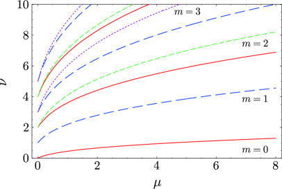
Figure 1: Angular eigenvalues for a conformal scalar field perturbations as a function of $\mu$. Different colors belong to different magnetic quantum numbers: $m=0$ (red solid lines), $m=1$ (blue long-dashed lines), $m=2$ (green dashed lines), $m=3$ (purple dotted lines).

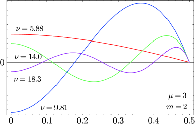
Figure 2: First several angular eigenmodes $S_{{\rm s}}(x)$ for $m=2$. The mass parameter is given by $\mu=3$.

Having thus determined the angular eigenvalues, we now move on to the analysis of the radial equation. Eq. (17) can be written in a familiar form using a “tortoise” coordinate

$$r_{*}:=r+2\mu\ell\ln\left(\frac{r}{2\mu\ell}-1\right),\quad r:=-\frac{\ell}{y}.$$ (20)

The black hole horizon is located at $y_{h}=-1/2\mu$ and hence is mapped to $r_{*}=-\infty$ ($r=2\mu\ell$), while the acceleration horizon $y=0$ corresponds to $r_{*}=+\infty$ ($r=+\infty$). In terms of $r_{*}$, we have the Schrödinger-type equation

$$\frac{{\rm d}^{2}}{{\rm d}r_{*}^{2}}R_{{\rm s}}+[\tilde{\omega}^{2}-V_{{\rm s}}(r)]R_{{\rm s}}=0,$$ (21)

where $\tilde{\omega}:=\omega/\ell$ and the potential is given by

$$V_{{\rm s}}(r)=\left(1-\frac{2\mu\ell}{r}\right)\left(\frac{\lambda}{r^{2}}+\frac{2\mu\ell}{r^{3}}\right).$$ (22)

It is important to note that Eq. (21) with the potential (22) is apparently identical to the radial equation for the (conformally coupled) scalar field perturbation in the 4D Schwarzschild background with the horizon radius $r_{h}=2\mu\ell$. The only change arises from the different angular eigenvalues.

In the asymptotically AdS spacetime, there is an ambiguity of the boundary conditions at infinity bc_AdS . In the present case, however, the chart of (1) covers only a part of the spacetime between the black hole and acceleration horizons. We thus impose the following quasinormal boundary conditions for the radial equation $R=R_{{\rm s}}$:

$$R\to\left\{\begin{array}[]{ll}e^{+i\tilde{\omega}r_{*}}&{\rm as}~{}~{}r_{*}\to\infty\\ e^{-i\tilde{\omega}r_{*}}&{\rm as}~{}~{}r_{*}\to-\infty\end{array}\right.,$$ (25)

having only an incoming wave at the black hole horizon and an outgoing wave at the acceleration horizon.

The QNMs of small localized black holes are approximately the same as those of 4D Schwarzschild ones since we have the eigenvalues $\nu\simeq 0,1,2,...$ for $\mu\ll 1$ and the same radial equation. This result accords with our intuition that if the horizon size of a localized black hole is much smaller than the bulk curvature radius, it behaves like a higher dimensional Schwarzschild black hole. Since $\nu$ becomes larger as $\mu$ increases, each mode of a large localized black hole behaves as if it were the mode having a larger angular mode number in the Schwarzschild background.

To evaluate the low-lying QNMs explicitly, we employ the WKB method developed by Iyer and Will IW . The third order WKB formula for the complex QNMs $\tilde{\omega}^{2}$ is given by IW (see also Konoplya:2003ii )

$$\tilde{\omega}^{2} = [V_{0}+(-2V_{0}^{\prime\prime})^{1/2}\tilde{\Lambda}]$$ (26)

$$\qquad-i(n+1/2)(-2V_{0}^{\prime\prime})^{1/2}(1+\tilde{\Omega}),$$

where $V_{0}$ is the maximum of the potential $V=V_{{\rm s}}$ and

$$\tilde{\Lambda} = \frac{1}{(-2V_{0}^{\prime\prime})^{1/2}}\Biggl{[}\frac{1}{8}\left(\frac{V_{0}^{(4)}}{V_{0}^{\prime\prime}}\right)\left(\frac{1}{4}+\alpha\right)$$ (27)

$$-\frac{1}{288}\left(\frac{V_{0}^{\prime\prime\prime}}{V_{0}^{\prime\prime}}\right)^{2}(7+60\alpha^{2})\Biggr{]},$$

$$\tilde{\Omega} = \frac{1}{(-2V_{0}^{\prime\prime})^{1/2}}\Biggl{[}\frac{5}{6912}\left(\frac{V_{0}^{\prime\prime\prime}}{V_{0}^{\prime\prime}}\right)^{4}(77+188\alpha^{2})$$ (28)

$$-\frac{1}{384}\left(\frac{V_{0}^{\prime\prime\prime 2}V_{0}^{(4)}}{V_{0}^{\prime\prime 3}}\right)(51+100\alpha^{2})$$

$$+\frac{1}{2304}\left(\frac{V_{0}^{(4)}}{V_{0}^{\prime\prime}}\right)^{2}(67+68\alpha^{2})$$

$$+\frac{1}{288}\left(\frac{V_{0}^{\prime\prime\prime}V_{0}^{(5)}}{V_{0}^{\prime\prime 2}}\right)(19+28\alpha^{2})$$

$$-\frac{1}{288}\left(\frac{V_{0}^{(6)}}{V_{0}^{\prime\prime}}\right)(5+4\alpha^{2})\Biggr{]}.$$

Here $\alpha:=n+1/2$, $n=0,1,2,...,$ (Re$\,[\omega]>0$), $-1,-2,-3,...,$ (Re$\,[\omega]<0$), and $V^{(n)}_{0}:={\rm d}^{n}V/{\rm d}r_{*}^{n}|_{0}$. The QNMs calculated using this formula are shown in Fig. 3. We have normalized the frequencies by (half of) the horizon radius: $\mu\ell\cdot\tilde{\omega}=\mu\omega$.

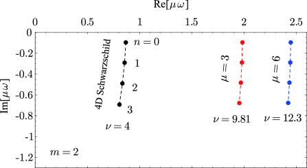
Figure 3: Conformal scalar QNMs for $m=2$. The plots are for the second lowest $\nu$ modes.

The WKB approximation will fail for higher overtones with $n>\nu$. The asymptotic QNMs ($n\gg 1$) are obtained using the monodromy method Motl ; MN2003 ; Andersson:2003fh ; Natario:2004jd ; Cho_asy (see Nollert ; Andersson ; CKL2003 for numerical calculations and Padmanabhan:2003fx for the other method). For a (conformal) scalar field in the Schwarzschild background, we have

$$\mu\omega_{n}\approx\frac{\ln 3}{8\pi}-\frac{i}{4}\left(n+\frac{1}{2}\right),$$ (29)

where one takes $n\to\infty$. This is independent of the angular eigenvalue and therefore the leading order behavior will be the same for the brane-localized and braneless black holes.

III.2 Massless Dirac field perturbations

Now we turn to the analysis of a massless, test Dirac field around the brane-localized black hole. The equation of motion for a massless Dirac field is given by

$$\gamma^{\alpha}e_{\alpha}^{\;a}(\partial_{a}+\Gamma_{a})\psi=0.$$ (30)

Here $e_{\alpha}^{\;a}$ is the tetrad defined by $g_{ab}=\eta_{\alpha\beta}e_{a}^{\;\alpha}e_{b}^{\;\beta}$, $\gamma^{\alpha}$ are the Dirac matrices

$$\gamma^{0}=\left(\begin{array}[]{cc}-i&0\\ 0&i\end{array}\right),\ \ \ \gamma^{i}=\left(\begin{array}[]{cc}0&-i\sigma^{i}\\ i\sigma^{i}&0\end{array}\right),$$ (35)

and $\Gamma_{a}$ is the spin connection given by

$$\Gamma_{a}=\frac{1}{8}[\gamma^{\alpha},\gamma^{\beta}]e_{\alpha}^{\;b}\nabla_{a}e_{\beta b},$$ (36)

with $\nabla_{a}e_{\beta b}=\partial_{a}e_{\beta b}-\Gamma^{c}_{ab}e_{\beta c}$. Under a conformal transformation (9) and

$$\psi \to \hat{\psi}=\Omega^{-3/2}\psi,$$ (37)

the Dirac equation (30) is invariant. Working in the conformally related metric $\hat{g}_{ab}$ and taking the conformally related tetrad to be

$$\hat{e}_{t}^{\;0}=\sqrt{-F},\;\;\hat{e}_{x}^{\;1}=\frac{1}{\sqrt{G}},\;\;\hat{e}_{\varphi}^{\;2}=\sqrt{G},\;\;\hat{e}_{y}^{\;3}=\frac{1}{\sqrt{-F}},$$

the field equation reduces to

$$\sqrt{-F}\left[-\frac{1}{F}\gamma^{0}\partial_{t}\hat{\psi}+(-F)^{-1/4}\gamma^{3}\partial_{y}\left((-F)^{1/4}\hat{\psi}\right)\right]$$

$$\quad+G^{1/4}\gamma^{1}\partial_{x}\left(G^{1/4}\hat{\psi}\right)+\frac{1}{\sqrt{G}}\gamma^{2}\partial_{\varphi}\hat{\psi}=0.$$ (38)

Following the argument of Ref. Cho , we assume the ansatz:

$$\hat{\psi}=\left(\begin{array}[]{c}iB(y)\chi_{1}(x)\\ A(y)\chi_{2}(x)\end{array}\right)(-FG)^{-1/4}e^{-i\omega t+im\varphi/\beta},$$ (41)

where

$$\chi_{1}=\left(\begin{array}[]{c}u\\ v\end{array}\right),\ \ \ \chi_{2}=\left(\begin{array}[]{c}u\\ -v\end{array}\right).$$ (46)

Note that for spinors the magnetic quantum eigenvalues must be half integers: $m=\pm 1/2,\pm 3/2,\pm 5/2,...\,$. Just for simplicity we assume in the following that $m>0$, but the case with negative $m$ can be treated analogously. After a straightforward calculation we arrive at

$$\sqrt{G}\frac{{\rm d}}{{\rm d}x}u-\frac{m/\beta}{\sqrt{G}}u = \kappa v,$$ (47)

$$\sqrt{G}\frac{{\rm d}}{{\rm d}x}v+\frac{m/\beta}{\sqrt{G}}v = -\kappa u,$$ (48)

and

$$\frac{{\rm d}}{{\rm d}y}A-\frac{\omega}{F}B = -\frac{\kappa}{\sqrt{-F}}A,$$ (49)

$$\frac{{\rm d}}{{\rm d}y}B+\frac{\omega}{F}A = \frac{\kappa}{\sqrt{-F}}B,$$ (50)

where $\kappa$ is a separation constant.

Equations (47) and (48) are combined to give a second-order differential equation

$$G\frac{{\rm d}^{2}}{{\rm d}x^{2}}u+\frac{G^{\prime}}{2}\frac{{\rm d}}{{\rm d}x}u+\left(\kappa^{2}+\frac{G^{\prime}}{2G}\frac{m}{\beta}-\frac{1}{G}\frac{m^{2}}{\beta^{2}}\right)u=0,$$ (51)

where $G^{\prime}:={\rm d}G/{\rm d}x$. The boundary condition at $x=x_{2}$ is derived in a similar way to the scalar field case by requiring the regularity of the function $\tilde{u}:=(x_{2}-x)^{-(m+1)/2}u$. To specify the boundary condition at the brane, let us change the variable $x\to x^{\prime}:=-x$ in Eqs. (47) and (48). Noting that the background has $Z_{2}$-symmetry and so $G(x^{\prime})=G(x)$, we find

$$\sigma^{1}\left(\begin{array}[]{c}u(x^{\prime})\\ v(x^{\prime})\end{array}\right)=\pm\left(\begin{array}[]{c}u(x)\\ v(x)\end{array}\right).$$ (56)

Thus, we impose either of

$$u(0)=+v(0)$$ (57)

or

$$u(0)=-v(0).$$ (58)

Let us first focus on the case of (57). We then integrate Eq. (51) to determine $\kappa$. Our numerical result is shown in Fig. 4. For $\mu\ll 1$ one finds that

$$\kappa \simeq ...\,,-m^{\prime}-4,\;-m^{\prime}-2,\;-m^{\prime},$$ (59)

$$\quad m^{\prime}+1,\;m^{\prime}+3,\;m^{\prime}+5,\;...\,,$$

where $m^{\prime}:=m+1/2$. Thus, in this limit the result for the 4D Schwarzschild black hole is reproduced (with half of the eigenmodes eliminated due to the brane boundary condition). We can see from Fig. 4 that $|\kappa|$ becomes larger as $\mu$ increases. If one instead imposes the condition (58), the spectrum will be such that

$$\kappa \simeq ...\,,-m^{\prime}-5,\;-m^{\prime}-3,\;-m^{\prime}-1,$$

$$\quad m^{\prime},\;m^{\prime}+2,\;m^{\prime}+4,\;...\,,$$

for $\mu\ll 1$ and $|\kappa|$ increases with increasing $\mu$. Note that the $\kappa=0$ mode is absent because it is not normalizable.

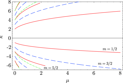
Figure 4: Angular eigenvalues $\kappa$ for a massless Dirac field perturbation as a function of $\mu$. The brane boundary condition is given by (57). Different colors belong to different magnetic quantum eigenvalues: $m=1/2$ (red solid lines), $m=3/2$ (blue long-dashed lines), $m=5/2$ (green dashed lines).

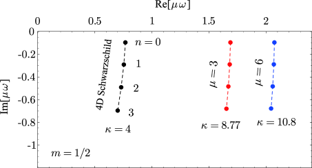
Figure 5: Massless Dirac QNMs for $m=1/2$. The plots are for the second lowest positive $\kappa$ modes. The brane boundary condition is given by (57).

In terms of $r_{*}$ and $r$ defined in Eq. (20), the radial equations (49) and (50) can be written as

$$\left(\frac{{\rm d}}{{\rm d}r_{*}}\pm W\right)\left(\begin{array}[]{c}A\\ B\end{array}\right)=\left(\begin{array}[]{c}-\tilde{\omega}B\\ +\tilde{\omega}A\end{array}\right),$$ (64)

where

$$W=\frac{\kappa}{r}\left(1-\frac{2\mu\ell}{r}\right)^{1/2}.$$ (65)

These equations can be decoupled, giving the Schrödinger-type equations

$$\frac{{\rm d}^{2}}{{\rm d}r_{*}^{2}}\left(\begin{array}[]{c}A\\ B\end{array}\right)+\left[\tilde{\omega}^{2}-V^{(\mp)}\right]\left(\begin{array}[]{c}A\\ B\end{array}\right)=0,$$ (70)

where

$$V^{(\pm)}=W^{2}\pm\frac{{\rm d}}{{\rm d}r_{*}}W.$$ (71)

The above equations are again the same as those for the massless Dirac field perturbations in 4D Schwarzschild spacetime. In particular, Eq. (71) implies that the potentials $V^{(+)}$ and $V^{(-)}$ are supersymmetric partners derived from the same superpotential $W$. Therefore, for these two potentials the QNMs and reflection/transmission amplitudes are the same Chandrasekhar .

The WKB result for the low-lying QNMs is shown in Fig. 5. With increasing $\mu$ one finds typically the same behavior of the low-lying modes as in the conformal scalar case. The asymptotic QNMs of Dirac field perturbations are the same as in the four-dimensional Schwarzschild case Cho :

$$\mu\omega_{n}\approx-i\frac{n}{4},$$ (72)

because the brane-localized and ordinary Schwarzschild black holes share the same potential and the asymptotic QNMs are independent of the angular eigenvalues.

III.3 Electromagnetic perturbations

Let us finally consider a test Maxwell field in the background of (1). It turns out that the situation is quite similar to the above two examples. The equations of motion are

$$\nabla_{a}F^{ab}=0,\quad\nabla_{[a}F_{bc]}=0,$$ (73)

where $F_{ab}:=\partial_{a}A_{b}-\partial_{b}A_{a}$. It follows from (73) that

$$\frac{1}{F}\partial_{t}^{2}\Phi_{p}-\partial_{y}\left[F\partial_{y}\Phi_{p}\right]$$

$$\qquad+\partial_{x}[G\partial_{x}\Phi_{p}]+\frac{1}{G}\partial_{\varphi}^{2}\Phi_{p}=0\quad(p={\rm N},{\rm D}),$$ (74)

where $\Phi_{\rm N}:=F_{ty}$ and $\Phi_{\rm D}:=F_{x\varphi}$. (We defer the details to appendix.) Assuming the separable ansatz $\Phi_{p}=e^{-i\omega t+im\varphi/\beta}R_{p}(y)S_{p}(x)$ for each $\Phi_{p}$, we obtain

$$\frac{{\rm d}}{{\rm d}x}\left[G(x)\frac{{\rm d}}{{\rm d}x}S_{p}\right]+\left[\nu(\nu+1)-\frac{m^{2}/\beta^{2}}{G(x)}\right]S_{p}=0,$$ (75)

$$\frac{{\rm d}}{{\rm d}y}\left[F(y)\frac{{\rm d}}{{\rm d}y}R_{p}\right]+\left[\nu(\nu+1)+\frac{\omega^{2}}{F(y)}\right]R_{p}=0,$$ (76)

To specify the boundary conditions at $x=x_{2}$, we make the transformation $S_{p}=(x_{2}-x)^{|m|/2}\tilde{S}_{p}$ and impose the regularity condition for each $\tilde{S}_{p}$. The brane boundary conditions are derived from

$$A_{x}|_{x=0}=\partial_{x}A_{i}|_{x=0}=0\quad(i=t,y,\varphi),$$

leading to the Neumann condition for $\Phi_{{\rm N}}$,

$$\left.\frac{{\rm d}S_{{\rm N}}}{{\rm d}x}\right|_{x=0}=0,$$ (77)

and the Dirichlet condition for $\Phi_{{\rm D}}$,

$$\left.S_{{\rm D}}\right|_{x=0}=0.$$ (78)

Now we can integrate the angular equation (75) numerically and determine the eigenvalues in much the same way as the earlier two examples. One sees from Figs. 6 and 7 that the qualitative behavior is the same as that of the conformal scalar field case: the angular eigenvalues increase with increasing $\mu$. It can be checked that for $\mu\ll 1$ we indeed have $\nu\simeq 1,2,3,...$, reproducing the 4D Schwarzschild result. Note the absence of the $\nu=m=0$ mode in the spectrum of spin-1 fields.

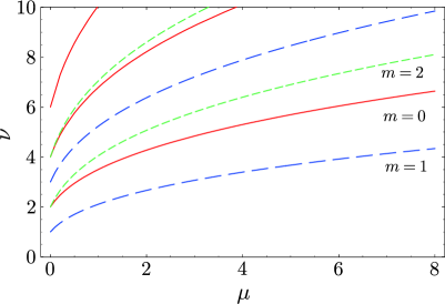
Figure 6: Angular eigenvalues for $\Phi_{{\rm N}}$ (which satisfies the Neumann boundary condition at the brane).

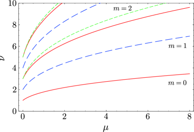
Figure 7: Angular eigenvalues for $\Phi_{{\rm D}}$ (which satisfies the Dirichlet boundary condition at the brane).

In terms of the tortoise coordinate $r_{*}$ defined by Eq. (20), the radial equation can be written in the same form as (21) but now with the potential given by

$$V_{{\rm em}}(r)=\left(1-\frac{2\mu\ell}{r}\right)\frac{\nu(\nu+1)}{r^{2}}.$$ (79)

Also in this case the potential is identical to that for electromagnetic perturbations in the 4D Schwarzschild black hole background. Again, the difference comes only from the different angular eigenvalues which have been determined in the above.

We will not dwell on the behavior of the electromagnetic QNMs because one can easily guess from the results of conformal scalar and Dirac field perturbations. The asymptotic QNMs are the same as that of the spin $1/2$ field (72) Cho_asy .

IV Conclusions

In this paper we have studied the QNMs of black holes localized on the Randall-Sundrum 2-brane. The background is the exact black hole solution found in Ref. EHM1 . The conformal properties of the solution allow us to obtain separable equations of motion for conformally invariant test fields. Taking advantage of this fact, we have investigated the behavior of conformal scalar, electromagnetic, and massless Dirac field perturbations around the brane-localized black hole.

For all types of fields we considered, we found that each radial equation is identical to the corresponding field equation in the 4D Schwarzschild background. However, the angular equations differ from their 4D Schwarzschild counterparts. We have determined the angular eigenfunctions and eigenvalues numerically. In the case of the conformal scalar field, the angular eigenvalues $\nu$ are given by $\nu\simeq l=0,1,2,...$ for a small black hole $(\mu\ll 1)$, recovering the 4D Schwarzschild result. However, the large localized black hole cannot be approximated by an isolated 4D Schwarzschild black hole. Indeed, as the size of the black hole increases, $\nu$ becomes larger ($\nu>l$) and no longer independent of the angular eigenvalue $m$. Accordingly, each QNM of the large localized black hole (with the horizon radius $2\mu\ell$ on the brane) behaves like the mode having a larger angular mode number in the 4D Schwarzschild background with the same horizon radius $r_{h}=2\mu\ell$. The situation is basically the same for electromagnetic and massless Dirac field perturbations. In particular, we have found no unstable modes for any types of fields we investigated.

Unfortunately, higher dimensional generalizations of the localized black holes of EHM1 ; EHM2 have not been known so far. There might even be no large, static black hole solutions localized on the Randall-Sundrum 3-brane Tanaka ; EFK , as mentioned in Introduction. Nevertheless, we believe it intriguing and important to show the stability of the configuration of a black hole intersected by a codimension-1 brane in AdS.

It has been widely known that the Randall-Sundrum braneworlds have a rich structure concerning the AdS/CFT correspondence. It would be also interesting to discuss the implications of our result from the viewpoint of the AdS/CFT correspondence. We hope to revisit this issue in the near future.

Appendix A More on electromagnetic perturbations

In this appendix we derive a set of governing equations for a test Maxwell field. We define convenient quantities

$$\Phi_{0}:=F_{ty}+iF_{x\varphi}$$ (80)

and

$$\Phi_{\pm}:= \frac{1}{F}\left(\sqrt{G}F_{tx}\pm\frac{i}{\sqrt{G}}F_{t\varphi}\right)$$

$$\quad\pm\left(\sqrt{G}F_{yx}\pm\frac{i}{\sqrt{G}}F_{y\varphi}\right).$$ (81)

The electromagnetic tensor $F_{ab}$ contains six independent real functions, and hence three complex scalars $\Phi_{0}$ and $\Phi_{\pm}$ are completely equivalent to $F_{ab}$.

It follows from the Maxwell equations (73) that

$${\cal L}_{\pm}\Phi_{0} ={\cal D}_{\mp}\sqrt{G}\Phi_{\pm},$$ (82)

$${\cal L}_{\mp}F\Phi_{\pm} =\sqrt{G}{\cal D}_{\pm}\Phi_{0},$$ (83)

where we defined the differential operators

$${\cal L}_{\pm} :=\pm\frac{1}{F}\partial_{t}+\partial_{y},$$ (84)

$${\cal D}_{\pm} :=\partial_{x}\pm\frac{i}{G}\partial_{\varphi}.$$ (85)

Note that ${\cal L}_{+}F{\cal L}_{-}={\cal L}_{-}F{\cal L}_{+}=-F^{-1}\partial_{t}^{2}+\partial_{y}F\partial_{y}$ and ${\cal D}_{+}G{\cal D}_{-}={\cal D}_{-}G{\cal D}_{+}=\partial_{x}G\partial_{x}+G^{-1}\partial_{\varphi}^{2}$. Equations (82) and (83) combine to give decoupled second order differential equations for $\Phi_{0}$ and $\Phi_{\pm}$:

$$-{\cal L}_{-}F{\cal L}_{+}\Phi_{0}+{\cal D}_{-}G{\cal D}_{+}\Phi_{0} =0,$$ (86)

$$-{\cal L}_{\pm}{\cal L}_{\mp}F\Phi_{\pm}+\sqrt{G}{\cal D}_{\pm}{\cal D}_{\mp}\sqrt{G}\Phi_{\pm} =0.$$ (87)

The first equation corresponds to Eq. (74) in the main text. To solve Eq. (86) it is convenient to expand $\Phi_{0}$ in terms of the eigenfunctions ${}_{0}{\cal Y}_{\nu m}(x,\varphi)$ satisfying

$${\cal D}_{-}G{\cal D}_{+}\,{}_{0}{\cal Y}_{\nu m}=-\lambda_{\nu m}\,{}_{0}{\cal Y}_{\nu m},$$ (88)

where $\lambda_{\nu m}$ is the eigenvalue. For $\Phi_{\pm}$ we may use the eigenfunctions ${}_{\pm}{\cal Y}_{\nu m}$ defined by

$${}_{\pm}{\cal Y}_{\nu m}:=\sqrt{G}{\cal D}_{\pm}\,{}_{0}{\cal Y}_{\nu m},$$ (89)

which satisfy the equation

$$\sqrt{G}{\cal D}_{\pm}{\cal D}_{\mp}\sqrt{G}\,{}_{\pm}{\cal Y}_{\nu m}=-\lambda_{\nu m}\,{}_{\pm}{\cal Y}_{\nu m}.$$ (90)

If Eq. (86) is solved, then the remaining fields $\Phi_{\pm}$ are obtained from Eq. (83).

References

- (1) N. Arkani-Hamed, S. Dimopoulos and G. R. Dvali, Phys. Lett. B 429, 263 (1998) [arXiv:hep-ph/9803315]; N. Arkani-Hamed, S. Dimopoulos and G. R. Dvali, Phys. Rev. D 59, 086004 (1999) [arXiv:hep-ph/9807344]; I. Antoniadis, N. Arkani-Hamed, S. Dimopoulos and G. R. Dvali, Phys. Lett. B 436, 257 (1998) [arXiv:hep-ph/9804398]; C. Kokorelis, Nucl. Phys. B 677, 115 (2004) [arXiv:hep-th/0207234].
- (2) L. Randall and R. Sundrum, Phys. Rev. Lett. 83, 3370 (1999) [arXiv:hep-ph/9905221]; L. Randall and R. Sundrum, Phys. Rev. Lett. 83, 4690 (1999) [arXiv:hep-th/9906064].
- (3) S. B. Giddings and S. D. Thomas, Phys. Rev. D 65, 056010 (2002) [arXiv:hep-ph/0106219]; S. Dimopoulos and G. L. Landsberg, Phys. Rev. Lett. 87, 161602 (2001) [arXiv:hep-ph/0106295]; S. Hossenfelder, S. Hofmann, M. Bleicher and H. Stoecker, Phys. Rev. D 66, 101502 (2002) [arXiv:hep-ph/0109085].
- (4) P. Kanti, Int. J. Mod. Phys. A 19, 4899 (2004) [arXiv:hep-ph/0402168].
- (5) N. Kaloper and D. Kiley, JHEP 0603, 077 (2006) [arXiv:hep-th/0601110]; D. Kiley, Phys. Rev. D 76, 126002 (2007) [arXiv:0708.1016 [hep-th]].
- (6) D. C. Dai, N. Kaloper, G. D. Starkman and D. Stojkovic, Phys. Rev. D 75, 024043 (2007) [arXiv:hep-th/0611184]; S. Chen, B. Wang and R. K. Su, Phys. Lett. B 647, 282 (2007) [arXiv:hep-th/0701209]; U. A. al-Binni and G. Siopsis, arXiv:0708.3363 [hep-th]; H. T. Cho, A. S. Cornell, J. Doukas and W. Naylor, arXiv:0710.5267 [hep-th]; T. Kobayashi, M. Nozawa and Y. i. Takamizu, Phys. Rev. D 77, 044022 (2008) [arXiv:0711.1395 [hep-th]]; D. C. Dai, G. Starkman, D. Stojkovic, C. Issever, E. Rizvi and J. Tseng, arXiv:0711.3012 [hep-ph].
- (7) A. Flachi, O. Pujolas, M. Sasaki and T. Tanaka, Phys. Rev. D 74, 045013 (2006) [arXiv:hep-th/0604139]; A. Flachi and T. Tanaka, Phys. Rev. Lett. 95, 161302 (2005) [arXiv:hep-th/0506145]; A. Flachi and T. Tanaka, Phys. Rev. D 76, 025007 (2007) [arXiv:hep-th/0703019]; V. P. Frolov and D. Stojkovic, Phys. Rev. D 66, 084002 (2002) [arXiv:hep-th/0206046]; V. P. Frolov, M. Snajdr and D. Stojkovic, Phys. Rev. D 68, 044002 (2003) [arXiv:gr-qc/0304083]; V. P. Frolov, D. V. Fursaev and D. Stojkovic, Class. Quant. Grav. 21, 3483 (2004) [arXiv:gr-qc/0403054]; V. P. Frolov, D. V. Fursaev and D. Stojkovic, JHEP 0406, 057 (2004) [arXiv:gr-qc/0403002].
- (8) P. Kanti and K. Tamvakis, Phys. Rev. D 65, 084010 (2002) [arXiv:hep-th/0110298]; P. Kanti, I. Olasagasti and K. Tamvakis, Phys. Rev. D 68, 124001 (2003) [arXiv:hep-th/0307201].
- (9) H. Kudoh, T. Tanaka and T. Nakamura, Phys. Rev. D 68, 024035 (2003) [arXiv:gr-qc/0301089].
- (10) T. Tanaka, Prog. Theor. Phys. Suppl. 148, 307 (2003) [arXiv:gr-qc/0203082].
- (11) R. Emparan, A. Fabbri and N. Kaloper, JHEP 0208, 043 (2002) [arXiv:hep-th/0206155].
- (12) T. Tanaka, arXiv:0709.3674 [gr-qc].
- (13) N. Tanahashi and T. Tanaka, JHEP 0803, 041 (2008) [arXiv:0712.3799 [gr-qc]].
- (14) R. Gregory, S. F. Ross and R. Zegers, arXiv:0802.2037 [hep-th].
- (15) S. Creek, R. Gregory, P. Kanti and B. Mistry, Class. Quant. Grav. 23 (2006) 6633 [arXiv:hep-th/0606006].
- (16) R. Emparan, G. T. Horowitz and R. C. Myers, JHEP 0001, 007 (2000).
- (17) R. Emparan, G. T. Horowitz and R. C. Myers, JHEP 0001, 021 (2000) [arXiv:hep-th/9912135].
- (18) M. Anber and L. Sorbo, arXiv:0803.2242 [hep-th].
- (19) H. Kodama, arXiv:0804.3839 [hep-th].
- (20) K. D. Kokkotas and B. G. Schmidt, Living Rev. Rel. 2, 2 (1999) [arXiv:gr-qc/9909058].
- (21) H. P. Nollert, Class. Quant. Grav. 16 (1999) R159.
- (22) P. Kanti and R. A. Konoplya, Phys. Rev. D 73, 044002 (2006) [arXiv:hep-th/0512257]; P. Kanti, R. A. Konoplya and A. Zhidenko, Phys. Rev. D 74, 064008 (2006) [arXiv:gr-qc/0607048];
- (23) V. Cardoso, J. P. S. Lemos and S. Yoshida, Phys. Rev. D 69, 044004 (2004) [arXiv:gr-qc/0309112];
- (24) R. A. Konoplya, Phys. Rev. D 68, 124017 (2003) [arXiv:hep-th/0309030];
- (25) R. A. Konoplya, Phys. Rev. D 68, 024018 (2003) [arXiv:gr-qc/0303052].
- (26) G. T. Horowitz and V. E. Hubeny, Phys. Rev. D 62, 024027 (2000) [arXiv:hep-th/9909056]; D. Birmingham, I. Sachs and S. N. Solodukhin, Phys. Rev. Lett. 88, 151301 (2002) [arXiv:hep-th/0112055]; D. Birmingham, Phys. Rev. D 64, 064024 (2001) [arXiv:hep-th/0101194]; P. K. Kovtun and A. O. Starinets, Phys. Rev. D 72, 086009 (2005) [arXiv:hep-th/0506184]; D. Birmingham, I. Sachs and S. N. Solodukhin, Phys. Rev. D 67, 104026 (2003) [arXiv:hep-th/0212308].
- (27) V. Cardoso and J. P. S. Lemos, Phys. Rev. D 64, 084017 (2001) [arXiv:gr-qc/0105103]. V. Cardoso and J. P. S. Lemos, Class. Quant. Grav. 18, 5257 (2001) [arXiv:gr-qc/0107098]; V. Cardoso and J. P. S. Lemos, Phys. Rev. D 63, 124015 (2001) [arXiv:gr-qc/0101052]; J. S. F. Chan and R. B. Mann, Phys. Rev. D 55, 7546 (1997) [arXiv:gr-qc/9612026]; J. S. F. Chan and R. B. Mann, Phys. Rev. D 59, 064025 (1999).
- (28) R. Emparan, JHEP 0606, 012 (2006) [arXiv:hep-th/0603081].
- (29) A. L. Dudley and J. D. Finley, III, Phys. Rev. Lett. 38, 1505 (1977).
- (30) G. F. Torres del Castillo, J. Math. Phys. 35, 3051 (1994).
- (31) S. W. Hawking and S. F. Ross, Phys. Rev. D 56, 6403 (1997) [arXiv:hep-th/9705147].
- (32) W. Kinnersley and M. Walker, Phys. Rev. D 2, 1359 (1970); J. F. Plebanski and M. Demianski, Annals Phys. 98 (1976) 98.
- (33) B. Carter, Commun. Math. Phys. 10 (1968) 280; B. Carter, Phys. Rev. D 16 (1977) 3395.
- (34) P. Breitenlohner and D. Z. Freedman, Phys. Lett. B 115, 197 (1982); P. Breitenlohner and D. Z. Freedman, Annals Phys. 144, 249 (1982); A. Ishibashi and R. M. Wald, Class. Quant. Grav. 21, 2981 (2004) [arXiv:hep-th/0402184].
- (35) S. Iyer and C. M. Will, Phys. Rev. D 35, 3621 (1987).
- (36) L. Motl, Adv. Theor. Math. Phys. 6, 1135 (2003) [arXiv:gr-qc/0212096].
- (37) L. Motl and A. Neitzke, Adv. Theor. Math. Phys. 7, 307 (2003) [arXiv:hep-th/0301173].
- (38) N. Andersson and C. J. Howls, Class. Quant. Grav. 21, 1623 (2004) [arXiv:gr-qc/0307020].
- (39) J. Natario and R. Schiappa, Adv. Theor. Math. Phys. 8, 1001 (2004) [arXiv:hep-th/0411267].
- (40) H. T. Cho, Phys. Rev. D 73, 024019 (2006) [arXiv:gr-qc/0512052].
- (41) H-P. Nollert, Phys. Rev. D 47, 5253 (1993);
- (42) N. Andersson, Class. Quant. Grav. 10, L61 (1993).
- (43) V. Cardoso, R. Konoplya and J. P. S. Lemos, Phys. Rev. D 68, 044024 (2003) [arXiv:gr-qc/0305037].
- (44) T. Padmanabhan, Class. Quant. Grav. 21, L1 (2004) [arXiv:gr-qc/0310027].
- (45) H. T. Cho, Phys. Rev. D 68, 024003 (2003) [arXiv:gr-qc/0303078]. H. T. Cho, A. S. Cornell, J. Doukas and W. Naylor, Phys. Rev. D 75, 104005 (2007) [arXiv:hep-th/0701193].
- (46) S. Chandrasekhar, The Mathematical Theory of Black Holes, (Oxford University Press, New York, 1983).