Pionic contribution to relativistic Fermi Liquid parameters

Abstract

We calculate pionic contribution to the relativistic Fermi Liquid parameters (RFLPs) using Chiral Effective Lagrangian. The RFLPs so determined are then used to calculate chemical potential, exchange and nuclear symmetry energies due to $\pi$$N$ interaction. We also evaluate two loop ring diagrams involving $\sigma$, $\omega$ and $\pi$ meson exchanges and compare results with what one obtains from the relativistic Fermi Liquid theory (RFLT).

I Introduction

Fermi liquid theory (FLT) provides us with one of the most important theoretical scheme to study the properties of strongly interacting Fermi systems involving low lying excitations near the Fermi surface song01 . Although developed originally in the context of studying the properties of ${}^{3}He$, it has widespread applications in other disciplines of many body physics like superconductivity, super fluidity, nuclear and neutron star matter etc baym_book ; chin76 .

In nuclear physics FLT was first extended and used by Migdal migdal78 to study the properties of both unbound nuclear matter and Finite nuclei mig_book . FLT also provides theoretical foundation for the nuclear shell model mig_book as well as nuclear dynamics of low energy excitationsbaym_book ; krewald88 . Particularly, ref.brown71 reveals the connection between Landau, Brueckner-Bethe and Migdal theories, ref.celenza_book ; anastasio83 , on the other hand, calculates the Migdal parameters using one-boson-exchange models of the nuclear force and shows how these parameters are modified if nuclear matter is considered within the context of Relativistic Brueckner-Hartree-Fock (RBHF) model. Some of the recent work that examines Fermi-liquid properties of hadronic matter also incorporates Brown-Rho (BR) scaling which is very important for the study of the properties of hadrons in dense nuclear matter (DNM)friman96 ; friman99 .

Most of the earlier nuclear matter calculations that involved Landau theory were done in a non-relativistic framework. The relativistic extension of the FLT was first developed by Baym and Chin chin76 in the context of studying the properties of DNM. In chin76 the authors invoked Walecka model (WM) to calculate various interaction parameters ($f_{pp^{\prime}}$) but did not consider mean fields (MF) for the $\sigma$ and $\omega$ meson i.e. there the FLPs are calculated perturbatively.

Later Matsui revisited the problem in matsui81 where one starts from the expression of energy density in presence of scalar and vector meson MF and takes functional derivatives to determine the FLPs. The results are qualitatively different than the perturbative results as may be seen from chin76 ; matsui81 . A comparison of relativistic and non-relativistic calculations have been made in celenza_book ; anastasio83 which also discusses how the FLPs are modified in presence of the $\sigma$ and $\omega$ MF and contrast those with perturbative results.

Besides $\sigma$ and $\omega$ meson, ref.matsui81 also includes the $\rho$ and $\pi$ meson and the model adopted was originally proposed by Serot to incorporate pion into the WM. It is to be noted, however, that the FLPs presented in matsui81 are independent of $\pi$ meson. This is because $\pi$, being a pseudoscalar, fails to contribute at the MF level. Hence to estimate the pionic contribution to FLPs it is necessary to go beyond MF formalism.

It is to be noted that, to our knowledge, such relativistic calculations including $\pi$ exchange does not exist, despite the fact that pion has a special status in nuclear physics as it is responsible for the spin-isospin dependent long range nuclear force. Furthermore, there are various non-relativistic calculations including the celebrated work of Migdal which shows that the pionic contribution to FLPs are important friman96 ; friman99 ; rho80 and most dominant for low energy excitations. It might be mentioned here that friman99 discusses how can one incorporate relativistic corrections to $F_{1}^{\pi}$ in the static potential model calculation. We, however, take the approach of chin76 where all the fields are treated relativistically.

The other major departure of the present work from ref.chin76 ; matsui81 resides in the choice of model for the description of the many body nuclear system. Unlike previous calculations chin76 ; matsui81 , here we use recently developed Chiral Effective Field Theory (chEFT) to calculate the RFLPs. Such a choice is motivated by the following earlier works that we now briefly review.

The first attempt to include $\pi$ and $\rho$ meson into the WM was made in serot79 where to describe the $\pi$N dynamics pseudoscalar (PS) coupling was used. Such straightforward inclusion of $\pi$ meson into the WM has serious difficulties. In particular, at the MF level it gives rise to tachyonic mode in matter at densities as low as $0.1\rho_{0}$, where $\rho_{0}$ is the nuclear saturation density kapusta81 . Inclusion of exchange diagrams removes such unphysical mode but makes the effective mass unrealistically large. If one simply replaces the PS coupling of ref.serot79 with the pseudovector (PV) interaction, these difficulties can be avoided. This, however, turns the theory non-renormalizable serot82 .

In serot82 it was shown how, starting from a PS coupling one can arrive at PV representation which preserves renormalizibility of the theory and at the same time yields realistic results for the pion dispersion relations in matter. But this model was also not found to be trouble free, particularly it had several shortcomings in describing $\pi$$N$ dynamics in matter which we do not discuss here and refer the reader to furnstahl87 ; furnstahl93 ; furnstahl95 ; furnstahl96 ; serot97 ; biswas08 .

Furthermore, the WM itself has several problems in relation to convergence which forbids systematic expansion scheme to perform any perturbative calculations. This was first exposed in ref.furnstahl89 .

The most recent model that provides us with a systematic scheme to study the dense nuclear system is provided by chEFT serot97 ; furnstahl89 ; furnstahl97 ; hu07 where the criterion of renormalizibility is given up in favor of successful relativistic description of DNM and the properties of finite nuclei. The chEFT, apart from $\sigma$ and $\omega$ mesons, also includes pion and therefore is best suited for the present purpose.

In this paper we estimate contributions of pion exchange to the FLPs within the framework of RFLT and subsequently use the parameters so determined to calculate various quantities like pionic contribution to the chemical potential, energy density, symmetry energy ($\beta$) etc. For completeness and direct comparison with the two loop results we also calculate here the exchange energy due to the interaction mediated by the $\sigma$, $\omega$ and $\pi$ mesons.

II Formalism

Now we quickly outline the formalism. In FLT the energy density $E$ of an interacting system is the functional of occupation number $n_{p}$ of the quasi-particle states of momentum $p$. The excitation of the system is equivalent to the change of occupation number by an amount $\delta n_{p}$. The corresponding energy of the system is given by baym_book ; chin76 ,

$${}E = E^{0}+\sum_{s}\int\frac{d^{3}{p}}{(2\pi)^{3}}\varepsilon_{ps}^{0}\delta n_{ps}$$ (1)

$$+\frac{1}{2}\sum_{ss^{\prime}}\int\frac{d^{3}{p}}{(2\pi)^{3}}\frac{d^{3}{p^{\prime}}}{(2\pi)^{3}}f_{ps,p^{\prime}s^{\prime}}\delta n_{ps}\delta n_{p^{\prime}s^{\prime}}.$$

Here, $s$ is the spin index. The quasi-particle energy can be written as,

$$\varepsilon_{ps}=\varepsilon_{ps}^{0}+\sum_{s^{\prime}}\int\frac{d^{3}{p^{\prime}}}{(2\pi)^{3}}f_{ps,p^{\prime}s^{\prime}}\delta n_{p^{\prime}s^{\prime}},$$ (2)

where superscript $0$ denotes the ground state baym_book . It is to be remembered, that, although the interaction ($f_{ps,p^{\prime}s^{\prime}}$) between the quasiparticles is not small, the problem is greatly simplified because it is sufficient to consider only pair collisions between the quasiparticles mig_book .

Since quasi-particles are well defined only near the Fermi surface, one assumes

$$\left.\begin{array}[]{lll}&\varepsilon_{p}&=\mu+v_{f}(p-p_{f})\\ {\rm and}{}{}{}&p&\simeq p^{\prime}\simeq p_{f}.\end{array}\right\}$$ (5)

Then LPs $f_{l}$s are defined by the Legendre expansion of $f_{ps,p^{\prime}s^{\prime}}$ as baym_book ; chin76 ,

$$f_{l}=\frac{2l+1}{4}\sum_{ss^{\prime}}\int\frac{d\Omega}{4\pi}P_{l}(\cos\theta)f_{ps,p^{\prime}s^{\prime}}$$ (6)

where $\theta$ is the angle between $p$ and $p^{\prime}$, both taken to be on the Fermi surface, and the integration is over all directions of $p$. We restrict ourselves for $l\leq 1$ i.e. $f_{0}$ and $f_{1}$, as higher $l$ contribution decreases rapidly chin76 ; matsui81 .

Now the Landau Fermi liquid interaction $f_{ps,p^{\prime}s^{\prime}}$ is related to the two particle forward scattering amplitude via chin76 ,

$$f_{ps,p^{\prime}s^{\prime}} = \frac{M}{\varepsilon_{p}^{0}}\frac{M}{\varepsilon_{p^{\prime}}^{0}}{\cal M}_{ps,p^{\prime}s^{\prime}},$$ (7)

where the Lorentz invariant matrix ${\cal M}_{ps,p^{\prime}s^{\prime}}$ consists of the usual direct and exchange amplitude, which may be evaluated directly from the relevant Feynman diagrams. The spin averaged scattering amplitude $(f_{pp^{\prime}})$ is given by chin76 ,

$$f_{pp^{\prime}} = \frac{1}{4}\sum_{ss^{\prime}}\frac{M}{\varepsilon_{p}^{0}}\frac{M}{\varepsilon_{p^{\prime}}^{0}}{\cal M}_{ps,p^{\prime}s^{\prime}}.$$ (8)

The dimensionless LPs are $F_{l}=N(0)f_{l}$, where $N(0)$ is the density of states at the Fermi surface defined as matsui81 ,

$$N(0) = \frac{g_{s}g_{I}p_{f}\varepsilon_{f}}{2\pi^{2}}.$$ (9)

Here $g_{s},g_{I}$ are the spin and isospin degeneracy factor respectively.

III Landau Parameters

By retaining only the lowest order terms in the pion fields, one obtains the following Lagrangian from the chirally invariant Lagrangian furnstahl97 ; hu07 :

$${\cal{L}} = \bar{\Psi}\left[\gamma^{\mu}(i\partial_{\mu}-g_{\omega}\omega_{\mu})-i\frac{g_{A}}{f_{\pi}}\gamma^{\mu}\gamma_{5}\partial_{\mu}\underline{\pi}-(M-g_{\sigma}\Phi_{\sigma})\right]\Psi$$ (10)

$$+\frac{1}{2}\partial^{\mu}\Phi_{\sigma}\partial_{\mu}\Phi_{\sigma}-\frac{1}{2}m_{\sigma}^{2}\Phi_{\sigma}^{2}-\frac{1}{4}\omega^{\mu\nu}\omega_{\mu\nu}+\frac{1}{2}m_{\omega}^{2}\omega^{\mu}\omega_{\mu}$$

$$+\frac{1}{2}\partial^{\mu}{\vec{\Phi}_{\pi}}\cdot\partial_{\mu}{\vec{\Phi}_{\pi}}-\frac{1}{2}m_{\pi}^{2}{\vec{\Phi}_{\pi}^{2}}+{\cal{L}}_{NL}+\delta{\cal{L}},$$

where $\omega_{\mu\nu}=\partial_{\mu}\omega_{\nu}-\partial_{\nu}\omega_{\mu}$, $\underline{\pi}=\frac{1}{2}({\vec{\tau}}\cdot{\vec{\Phi}_{\pi}})$ and ${\vec{\tau}}$ is the isospin index. Here $\Psi$ is the nucleon field and $\Phi_{\sigma}$, $\omega_{\mu}$ and $\Phi_{\pi}$ are the meson fields (isoscalar-scalar, isoscalar-vector and isovector-pseudoscalar respectively). The terms ${\cal{L}}_{NL}$ and $\delta{\cal{L}}$ contain the non-linear and counterterms respectively (for explicit expressions see hu07 ).

Now due to presence of pion fields in the chiral Lagrangian we have component in the interaction which acts on the isospin fluctuation. One can derive the isospin dependent quasiparticle interaction along the line of ref.chin76 . For pions, as mentioned before, the direct term vanishes and it is only the exchange diagram that contributes to the interaction parameter :

$$f_{pp^{\prime}}^{ex,\pi}{\bigg{|}}_{p\simeq p^{\prime}=p_{f}} = \frac{3}{2}\frac{g_{A}^{2}M^{*2}}{4f_{\pi}^{2}\varepsilon_{f}^{2}}\left\{\frac{p_{f}^{2}(1-\cos\theta)}{2p_{f}^{2}(1-\cos\theta)+m_{\pi}^{2}}\right\},$$ (11)

where $\varepsilon_{f}=(p_{f}^{2}+M^{*^{2}})^{1/2}$ and $g_{A}^{2}=1.5876$ , $f_{\pi}=93MeV$, $m_{\pi}=139$ MeVhu07 . The factor $3/2$ arises since the isospin factor is $3/2$ in the isoscalar channel friman99 .

The effective nucleon mass $M^{*}$ is determined self-consistently from the following equation matsui81 ,

$$M^{*} = M-\frac{g_{\sigma}^{2}}{m_{\sigma}^{2}}{\sum_{i}}n_{i}\frac{M^{*}}{(p_{i}^{2}+M^{*2})^{1/2}}.$$ (12)

Using Eq.(6) and Eq.(11) we can derive isoscalar LPs $f_{0}^{ex,\pi}$ and $f_{1}^{ex,\pi}$,

$$f^{ex,\pi}_{0} = -\frac{3g_{A}^{2}M^{*2}}{32f_{\pi}^{2}\varepsilon_{f}^{2}}\left[-2+\frac{m_{\pi}^{2}}{2p_{f}^{2}}\ln\left(1+\frac{4p_{f}^{2}}{m_{\pi}^{2}}\right)\right],$$ (13)

and

$$\frac{1}{3}f^{ex,\pi}_{1} = -\frac{3g_{A}^{2}M^{*2}m_{\pi}^{2}}{64f_{\pi}^{2}\varepsilon_{f}^{2}p_{f}^{2}}\times$$ (14)

$$\left[-2+\left(\frac{m_{\pi}^{2}}{2p_{f}^{2}}+1\right)\ln\left(1+\frac{4p_{f}^{2}}{m_{\pi}^{2}}\right)\right].$$

Using Eqs.(13) and (14) we find that

$$f^{ex,\pi}_{0}-\frac{1}{3}f^{ex,\pi}_{1}=\frac{3g_{A}^{2}M^{*2}}{16f_{\pi}^{2}\varepsilon_{f}^{2}}\times$$

$$\left[\frac{m_{\pi}^{4}}{8p_{f}^{4}}\ln\left(1+\frac{4p_{f}^{2}}{m_{\pi}^{2}}\right)-\frac{m_{\pi}^{2}}{2p_{f}^{2}}+1\right].$$ (15)

It is this combination i.e. $f_{0}-\frac{1}{3}f_{1}$, which appears in the calculation of chemical potential and other relevant quantities. For the massless pion, Eq.(III) turns out to be finite,

$$\left(f^{ex,\pi}_{0}-\frac{1}{3}f^{ex,\pi}_{1}\right){\Bigg{|}}_{m_{\pi}\rightarrow 0} = \frac{3g_{A}^{2}M^{*2}}{16f_{\pi}^{2}\varepsilon_{f}^{2}}.$$ (16)

It is to be noted that, in the massless limit for $\sigma$ and $\omega$ meson, $f^{ex}_{0}$ and $f^{ex}_{1}$ diverge as shown in chin76 , in contrast for pion, even in the massless limit, these are finite. This is due to the presence of $(1-\cos\theta)$ in the numerator of Eq.(11) unlike $\sigma$ and $\omega$ meson.

The dimensionless LPs can be determined by equating the equation $F_{0}=N(0)f_{0}$ and $F_{1}=N(0)f_{1}$, where $N(0)$ is the density of states at the Fermi surface defined in Eq.(9). Thus the dimensionless parameters are

$$F^{ex,\pi}_{0}=-g_{s}g_{I}\frac{3g_{A}^{2}p_{f}M^{*2}}{64\pi^{2}f_{\pi}^{2}\varepsilon_{f}}\left[-2+\frac{m_{\pi}^{2}}{2p_{f}^{2}}\ln\left(1+\frac{4p_{f}^{2}}{m_{\pi}^{2}}\right)\right],$$ (17)

and

$$\frac{1}{3}F^{ex,\pi}_{1}=-g_{s}g_{I}\frac{3g_{A}^{2}m_{\pi}^{2}M^{*2}}{128\pi^{2}f_{\pi}^{2}p_{f}\varepsilon_{f}}\times$$

$$\left[-2+\left(\frac{m_{\pi}^{2}}{2p_{f}^{2}}+1\right)\ln\left(1+\frac{4p_{f}^{2}}{m_{\pi}^{2}}\right)\right].$$ (18)

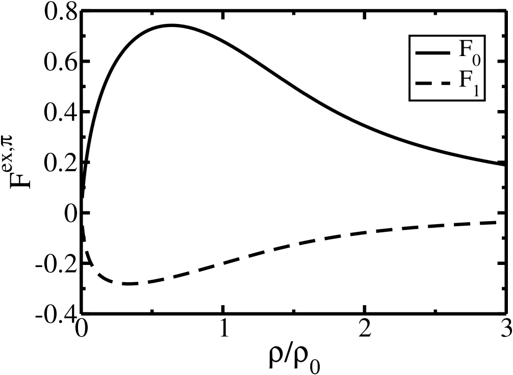
Figure 1: Dimensionless Landau parameters in symmetric nuclear matter for pion exchange in relativistic theory. Solid and dashed line represent $F_{0}$ and $F_{1}$ respectively.

In Fig.(1) we show the density dependent of $F_{0}$ and $F_{1}$ due to pionic interaction. Numerically at nuclear matter density $(\rho_{0}=0.148{\rm fm^{-3}})$, $F^{ex,\pi}_{0}=0.68$ and $F^{ex,\pi}_{1}=-0.2$. In the non-relativistic limit $\varepsilon_{f}\rightarrow M^{*}$, one obtains the same expression for $F_{1}^{\pi}$ as reported in friman96 ; rho80 .

IV Chemical potential

We now proceed to calculate the chemical potential which in principle will be different for the neutron and proton in asymmetric nuclear matter.

Although in the present work we deal with symmetric nuclear matter (SNM) for which $\mu_{p}=\mu_{n}$. To calculate the general expression for chemical potential with arbitrary asymmetry $(\alpha=(n_{n}-n_{p})/(n_{n}+n_{p}))$, we take distribution function with explicit isospin index $(b~{}or~{}b^{\prime})$, so that variation of distribution function gives baym_book

$$\delta n_{b} = -N_{b}(0)\left[\sum_{b^{\prime}}f_{0}^{bb^{\prime}}\delta n_{b^{\prime}}-\delta\mu_{b}\right],$$ (19)

where $N_{b}(0)$ is the isospin dependent density of states at the corresponding Fermi surface. The Eq.(19) yields

$$\frac{\partial\mu_{b}}{\partial n_{b}} = \frac{1}{N_{b}(0)}+\sum_{b^{\prime}}f_{0}^{bb^{\prime}}\frac{\partial n_{b^{\prime}}}{\partial n_{b}}.$$ (20)

In our case $b~{}(or~{}b^{\prime})=n,p$. Separately for neutron and proton we have

$$\left(\begin{array}[]{c}\partial{\mu_{n}}\\ \partial{\mu_{p}}\end{array}\right) = \left(\begin{array}[]{cc}\frac{1}{N_{n}(0)}+f_{0}^{nn}&f_{0}^{np}\\ f_{0}^{pn}&\frac{1}{N_{p}(0)}+f_{0}^{pp}\end{array}\right)\left(\begin{array}[]{c}\partial{n_{n}}\\ \partial{n_{p}}\end{array}\right),$$ (27)

where the superscripts $nn$ and $np$ denote neutron-neutron and neutron-proton quasiparticle interaction. $N_{n}(0)$ and $N_{p}(0)$ denote the density of states at neutron and proton Fermi surfaces respectively aguirre07 ; sjoberg76 . For pion exchange, in SNM, $f_{l}^{np(pn)}=2f_{l}^{nn(pp)}$ rho80 , from Eq.(27), we have,

$$\partial\mu_{n} = \frac{1+3F_{0}^{nn}}{N_{n}(0)}\partial n_{n},$$ (29)

where $F_{0}^{nn}=N_{n}(0)f_{0}^{nn}$. Similarly, one can determine $\partial\mu_{p}$. Motivated by mig_book , we define

$$f_{l}^{b} = \frac{1}{2}\sum_{b^{\prime}}f_{l}^{bb^{\prime}}.$$ (30)

Evidently in SNM, $f_{l}^{nn}=f_{l}^{pp}$, and therefore, we write $\mu_{n}=\mu_{p}=\mu$ chin76 ,

$$\mu{\rm d\mu}=\left[p_{f}+g_{s}g_{I}\frac{\mu p_{f}}{2\pi^{2}}\left(f_{0}-\frac{1}{3}f_{1}\right)\right]dp_{f}.$$ (31)

Here $f_{0}$ and $f_{1}$ are given by Eq.(13) and (14).

To calculate $\mu$, it is sufficient to let $\mu=\varepsilon_{f}$ in the right hand side of Eq.(31). With the constant of integration adjusted so that at high density $p_{f}\simeq\varepsilon_{f}$, Eq.(31) upon integration together with Eq.(III) yield

$$\mu = \varepsilon_{f}-g_{s}\frac{3g_{A}^{2}M^{*4}}{128\pi^{2}f_{\pi}^{2}\varepsilon_{f}}\times$$ (32)

$$\left[-2y_{\pi}^{3}\sqrt{-y_{\pi}^{2}+4}\tan^{-1}\left(\frac{x\sqrt{-y_{\pi}^{2}+4}}{y_{\pi}\sqrt{1+x^{2}}}\right)\right.$$

$$\left.+\frac{y_{\pi}^{4}\sqrt{1+x^{2}}}{x}\ln\left(1+\frac{4x^{2}}{y_{\pi}^{2}}\right)-4x\sqrt{1+x^{2}}\right.$$

$$\left.-2(y_{\pi}^{4}-2y_{\pi}^{2}-2)\ln(x+\sqrt{1+x^{2}})\right],$$

where $x=p_{f}/M^{*}$ and $y_{\pi}=m_{\pi}/M^{*}$.

The calculations of LPs for other mesons is straightforward. However, for brevity, we do not present corresponding expressions for $\sigma$ and $\omega$ mesons but quote their numerical values in Table(1). The numbers cited above are relevant for normal nuclear matter density $\rho_{0}=0.148{\rm fm^{-3}}$. For the coupling constants we adopt the same parameter set as designated by M0A in hu07 .

Interestingly, individual contribution to LPs of $\sigma$ and $\omega$ meson are large while sum of their contribution to $F_{0}^{tot}$ is small due to the sensitive cancellation of $F_{0}^{\sigma}$ and $F_{0}^{\omega}$ as can be seen from Table(1). Such a cancellation is responsible for the nuclear saturation dynamics celenza_book ; anastasio83 . Numerically, $F_{0}^{\sigma+\omega}$ is approximately $3/2$ times smaller than $F_{0}^{\pi}$.

Table 1: Dimensionless Landau parameters and chemical potential at $\rho=\rho_{0}$. Note that, $F_{0}$, $F_{1}$ are the dimensionless isoscalar LPs.

Meson	$F_{0}$	$F_{1}$
$\sigma$	-5.04	0.875
$\omega$	5.44	-0.93
$\pi$	0.68	-0.20

V Exchange energy

Once the $\mu$ is determined, one can readily calculate the energy density due to $\pi-N$ interaction in SNM as chin76 ; chin77 ,

$$E^{ex}_{\pi} = \int{\rm d\rho}(\mu-\varepsilon_{f})$$ (33)

$$= -g_{s}^{2}\frac{3g_{A}^{2}M^{*6}}{128f_{\pi}^{2}\pi^{4}}\times$$

$$\left[I_{\pi}+y_{\pi}^{4}\left\{-\frac{x^{2}}{2}+\frac{y_{\pi}^{2}+4x^{2}}{8}\ln\left(1+\frac{4x^{2}}{y_{\pi}^{2}}\right)\right\}-x^{4}\right.$$

$$\left.+\left(\frac{y_{\pi}^{4}}{2}-y_{\pi}^{2}-1\right)\left(\{x\eta-\ln(x+\eta)\}^{2}-x^{4}\right)\right],$$

where $\eta=\sqrt{1+x^{2}}$ and

$$I_{\pi}=-2y_{\pi}^{3}\sqrt{4-y_{\pi}^{2}}\int\frac{x^{2}}{\eta}\tan^{-1}\left(\frac{x\sqrt{4-y_{\pi}^{2}}}{y_{\pi}\eta}\right){\rm d}x.$$ (34)

For the massless pion this reads as

$$E^{ex}_{\pi}{\Big{|}}_{m_{\pi}\rightarrow 0} = \frac{3g_{A}^{2}M^{*6}}{32f_{\pi}^{2}\pi^{4}}[x\eta-\ln(x+\eta)]^{2}.$$ (35)

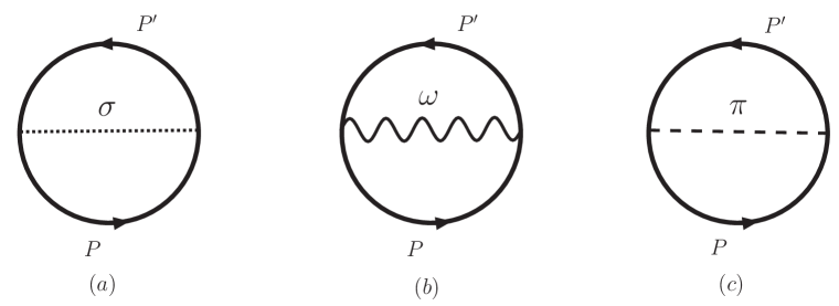
Figure 2: Two-loop contributions to the nuclear matter energy density. The solid line represents the baryon propagator. $\sigma$, $\omega$ and $\pi$ mesons are denoted by dotted, wavy and dashed line respectively.

The contribution arising from pion exchange from the direct evaluation of Fig.2(c) reads as hu07 ,

$$E^{ex}_{\pi}=g_{s}g_{I}\frac{3g_{A}^{2}}{32\pi^{4}f_{\pi}^{2}}M^{*2}\int_{0}^{p_{f}}\frac{|p|^{2}{\rm dp}}{\varepsilon_{p}}\int_{0}^{p_{f}}\frac{|p^{\prime}|^{2}{\rm dp^{\prime}}}{\varepsilon_{p^{\prime}}}\times$$

$$\int_{-1}^{1}{\rm d(\cos\theta)}\left[\frac{\varepsilon_{p}\varepsilon_{p^{\prime}}-|p||p^{\prime}|\cos\theta-M^{*2}}{2\varepsilon_{p}\varepsilon_{p^{\prime}}-2|p||p^{\prime}|\cos\theta-2M^{*2}+m_{\pi}^{2}}\right].$$ (36)

Similarly, from Fig.2-((a),(b)) one can determine exchange energy due to $\sigma$ and $\omega$ meson interaction hu07 . In Table(2) we given the exchange energy results calculated from RFLPs which is in agreement with two-loop results hu07 . It might be mentioned here that in the limit $m_{\pi}\rightarrow 0$, the Eq.(V) can be evaluated analytically which reproduces the Eq.(35) derived in FLT approach.

Table 2: Exchange energy in MeV from FLT at $\rho=\rho_{0}$.

Meson	$E^{ex}$
	FLT
$\sigma$	40.48
$\omega$	-23.41
$\pi$	12.49

VI Symmetry energy

Knowing the ”isovector” combination of the LPs, one can determine nuclear symmetry energy. The symmetry energy is defined as the difference of energy between the neutron matter and symmetric nuclear matter is given by the following expression matsui81 ; greco03

$$\beta = \frac{1}{2}\rho\frac{\partial^{2}E}{\partial\rho_{3}^{2}}{\bigg{|}}_{\rho_{3}=0}.$$ (37)

In terms of LPs, the symmetry energy can be expressed as mig_book

$$\beta=\frac{p_{f}^{2}}{6\varepsilon_{f}}(1+2F^{\prime}_{0}),$$ (38)

where $F_{0}^{\prime}=\frac{1}{2}(F_{0}^{nn}-F_{0}^{np})$ is the isovector combination of dimensionless Landau parameters $F_{0}$ mig_book ; greco03 . Deriving $F_{0}^{\prime}$, one can find symmetry energy. Numerically at saturation density ($\rho=\rho_{0}$) we obtain $\beta=14.57$ MeV. So relatively small contribution to $\beta$ comes from one pion exchange diagram dieper03

VII Summary and conclusion

In this paper, we calculate RFLPs within the framework of RFLT. For the description of dense nuclear system chEFT is invoked. Although our main focus was to estimate the contribution of pions to RFLPs, for comparison and completeness we also present results for the $\sigma$ and $\omega$ meson. It is seen that the pionic contribution to the FLPs are significantly larger compared to the combined contributions of $\sigma$ and $\omega$ meson. Thus any realistic relativistic calculation for the FLPs should include $\pi$ meson which necessarily implies going beyond the MF calculations. The LPs what we determine here are subsequently used to calculate exchange and symmetry energy of the system. Finally we evaluate two loop ring diagrams with the same set of interaction parameters and show that the numerical results are consistent with those obtained from the FLT. It might be mentioned here that in the present calculation we have ignored nucleon-nucleon correlations which might be worthwhile to investigate. It should, however, be noted that inclusion of correlation energy would require the readjustment of the coupling parameter so as to reproduce the saturation properties of nuclear matter.

Acknowledgments

The author would like to thank G.Baym and C.Gale for their valuable comments. I also wish to thank A.K.Dutt-Mazumder for the critical reading of the manuscript.

References

- (1) C.Song, Phys.Rept.347, 289 (2001).
- (2) G.baym and C.Pethick, Landau Fermi liquid Theory:Concepts and Applications, United States Of America (1991).
- (3) G.Baym and S.A.Chin, Nucl.Phys.A262, 527 (1976).
- (4) A.B.Migdal, Rev.Mod.Phys.50, 107 (1978).
-
(5)
A.B.Migdal, Theory of Finite Fermi Systems (1967)
(Wiley, New York) (Russ.ed.1965),
A.B.Migdal, Nuclear Theory: The Quasiparticle Method (1968) (Benjamin, New York). - (6) S.Krewald, K.Nakayama and J.Speth, Phys.Rept. 161, 103-170 (1988).
- (7) G.E.Brown, Rev.Mod.Phys.43, 1 (1971).
- (8) L.S.Celenza and C.M.Shakin, Relativistic Nuclear Physics(1986) (World Scientific, USA)
- (9) M.R.Anastasio, L.S.Celenza, W.S.Pong and C.M.Shakin, Phys.Rept.100, 327-392 (1983).
- (10) B.Friman and M.Rho, Nucl.Phys.A606, 303-319 (1996).
- (11) B.Friman, M.Rho and C.Song, Phys.Rev.C59, 3357-3370 (1999).
- (12) T.Matsui, Nucl.Phys.A370, 365 (1981).
- (13) G.E.Brown and M.Rho, Nucl.Phys.A338, 269 (1980).
- (14) B.D.Serot, Phys.Lett.B86 146 (1979); Erratum, Phys.Lett B87, 403 (1979).
- (15) J.I.Kapusta, Phys.Rev.C23, 1648 (1981).
- (16) T.Matsui and B.D.Serot, Annals of Physics 144, 107-167 (1982).
- (17) R.J.Furnstahl, C.E.Price and G.E.walker, Phys.Rev.C36, 2590 (1987).
- (18) R.J.Furnstahl and B.D.Serot, Phys.Lett.B316, 12 (1993).
- (19) R.J.Furnstahl, H.B.Tang and B.D.Serot, Phys.Rev.C52, 1368 (1995).
- (20) R.J.Furnstahl, B.D.Serot and H.B.Tang, Nucl.Phys. A598, 539 (1996).
- (21) B.D.Serot and J.D.Walecka, Int.J.Mod.Phys.E6, 515 (1997).
- (22) S.Biswas and A.K.Dutt-Mazumder, Phys.Rev.C77, 045201 (2008).
- (23) R.J.Furnstahl, R.J.Perry, B.D.Serot, Phys.Rev.C40, 321 (1989).
-
(24)
R.J.Furnstahl, B.D.Serot and H.B.Tang,
Nucl.Phys.A615, 441 (1997),
R.J.Furnstahl, B.D.Serot and H.B.Tang, Nucl.Phys.A640, 505 (1998), Erratum. - (25) Y.Hu, J.McIntire, B.D.Serot, Nucl.Phys.A794, 187 (2007).
- (26) R.M.Aguirre and A.L.De Paoli, Phys.Rev.C75, 045207 (2007).
- (27) O.Sjoberg, Nucl.Phys.A265, 511 (1976).
- (28) S.A.Chin, Annals of Physics 108, 301 (1977).
- (29) V.Greco, M.colonna, M.Di Toro and F.Matera, Phys.Rev.C67, 015203 (2003).
- (30) A.E.L.Dieperink, Y.Dewulf, D.Van Neck, M.Waroquier and V.Rodin, Phys.Rev.C68, 064307 (2003).