A Local Mean Field Analysis
of Security Investments in Networks

Abstract

Getting agents in the Internet, and in networks in general, to invest in and deploy security features and protocols is a challenge, in particular because of economic reasons arising from the presence of network externalities. Our goal in this paper is to model and investigate the impact of such externalities on security investments in a network.

Specifically, we study a network of interconnected agents subject to epidemic risks such as viruses and worms where agents can decide whether or not to invest some amount to deploy security solutions. We consider both cases when the security solutions are strong (they perfectly protect the agents deploying them) and when they are weak. We make three contributions in the paper. First, we introduce a general model which combines an epidemic propagation model with an economic model for agents which captures network effects and externalities. Second, borrowing ideas and techniques used in statistical physics, we introduce a Local Mean Field (LMF) model, which extends the standard mean-field approximation to take into account the correlation structure on local neighborhoods. Third, we solve the LMF model in a network with externalities, and we derive analytic solutions for sparse random graphs of agents, for which we obtain asymptotic results. We find known phenomena such as free riders and tipping points. We also observe counter-intuitive phenomena, such as increasing the quality of the security technology can result in a decreased adoption of that technology in the network. In general, we find that both situations with strong and weak protection exhibit externalities and that the equilibrium is not socially optimal - therefore there is a market failure. Insurance is one mechanism to address this market failure. In related work, we have shown that insurance is a very effective mechanism [3, 4] and argue that using insurance would increase the security in a network such as the Internet.

1 Introduction

Users and computers in the Internet face a wide range of security risks. Of particular concern, are epidemic risks, such as those propagated by worms and viruses. Epidemic risks depend on the behavior of other entities in the network, such as whether or not those entities invest in security solutions to minimize their likelihood of being infected. Our goal in this paper is to analyze the strategic behavior of agents facing such epidemic risks.

The propagation of worms and viruses [16, 7], but also many other phenomena in the Internet such as the propagation of alerts and patches [14] or of routing updates [5], can be modeled using epidemic spreads through a network. As a result, there is now a vast body of literature on epidemic spreads over a network topology from an initial set of infected nodes to susceptible nodes. However, much of that work has focused on modeling and understanding the propagation of the epidemics proper, without considering the impact of network effects and externalities.

Recent work which did model such effects has been limited to the simple case of two agents, i.e. a two-node network. For example, reference [9] proposes a parametric game-theoretic model for such a situation. In the model, agents decide whether or not to invest in security and agents face a risk of infection which depends on the state of other agents. The authors show the existence of two Nash equilibria (all agents invest or none invests), and suggest that taxation or insurance would be ways to provide incentives for agents to invest (and therefore reach the "good" Nash equilibrium). However, their approach does not scale to the case of $N$ agents, and it does not handle various network topologies connecting those agents. Our work addresses precisely those limitations.

The rest of the paper is organized as follows. In Section 2, we describe our model for epidemic risks with network effects and externalities. In Section 3, we introduce our Local Mean Field Model (LMF) and state asymptotic results that can be obtained with LMF. In Section 4, we use the LMF model to examine both cases when agents invest in strong security solutions (which perfectly protect the agents deploying them against propagated risks) and in weak solutions. We find known phenomena such as free riders and tipping points [4]. We also observe counter-intuitive phenomena, such as increasing the quality of the security technology can result in a decreased adoption of that technology in the network. In Section 5, we discuss our results and conclude the paper.

2 A model for epidemic risks and network effects

2.1 Economic model for the agents

We model agents using the classical expected utility model, where agents attempt to maximize a utility function $u$. We assume that agents are rational and that they are risk averse, i.e. their utility function is concave (see Proposition 2.1 in [8]). Risk averse agents dislike mean-preserving spreads in the distribution of their final wealth.

We denote by $w$ the initial wealth of the agent. The risk premium $\pi$ is the maximum amount of money that one is ready to pay to escape a pure risk $X$, where a pure risk $X$ is a random variable such that $\mathbb{E}[X]=0$. The risk premium corresponds to an amount of money paid (thus decreasing the wealth of the agent from $w$ to $w-\pi$) which covers the risk; hence, $\pi$ is given by the following equation: $u[w-\pi]=\mathbb{E}[u[w+X]]$.

Each agent faces a potential loss $\ell$, which we take in this paper to be a fixed (non-random) value. We denote by $p$ the probability of loss or damage. There are two possible final states for the agent: a good state, in which the final wealth of the agent is equal to his initial wealth $w$, and a bad state in which the final wealth is $w-\ell$. If the probability of loss is $p>0$, the risk is clearly not a pure risk. The amount of money $m$ the agent is ready to invest to escape the risk is given by the equation: $pu[w-\ell]+(1-p)u[w]=u[w-m].$ We clearly have $m>p\ell$ thanks to the concavity of $u$. We can actually relate $m$ to the risk premium defined above:

$$m=p\ell+\pi[p].$$

An agent can invest some amount in self-protection, which in practice would reflect an investment in antivirus or anomaly detection solutions. If an agent decides to invest in self-protection, we say that the agent is in state $S$ (as in Safe or Secure). If the agent decides not to invest in self-protection, it is in state $N$ (Not safe). If the agent does not invest, its probability of loss is $p^{N}$. If it does invest, for an amount which we assume is a fixed amount $c$, then its loss probability is reduced and equal to $p^{S}<p^{N}$.

In state $N$, the expected utility of the agent is $p^{N}u[w-\ell]+(1-p^{N})u[w]$; in state $S$, the expected utility is $p^{S}u[w-\ell-c]+(1-p^{S})u[w-c]$. Using the definition of risk premium, we see that these quantities are equal to $u[w-p^{N}\ell-\pi[p^{N}]]$ and $u[w-c-p^{S}\ell-\pi[p^{S}]]$, respectively. Therefore, the optimal strategy is for the agent to invest in self-protection only if the cost for self-protection is less than the threshold

$$c<(p^{N}-p^{S})\ell+\pi[p^{N}]-\pi[p^{S}].$$ (1)

2.2 Epidemic model

We describe now our model for the epidemic risk. Agents are represented by vertices of a graph. We assume that an agent in state $S$ has a probability $p^{-}$ of direct loss and an agent in state $N$ has a probability $p^{+}$ of direct loss with $p^{+}\geq p^{-}$. Then any infected agent contaminates neighbors independently of each others with probability $q^{-}$ if the neighbor is in state $S$ and $q^{+}$ if the neighbor is in state $N$, with $q^{+}\geq q^{-}$.

Special cases of this model are examined in [10], where $q^{+}=q^{-}$, and in [12], where agents in state $S$ are completely secure and cannot be infected, i.e. $p^{-}=q^{-}=0$.

Let $G=(V,E)$ be a graph on a countable vertex set $V$. Agents are represented by vertices of the graph. For $i,j\in V$, we write $i\sim j$ if $(i,j)\in E$ and we say that agents $i$ and $j$ are neighbors. The state of agent $i$ is represented by $X_{i}$; agent $i$ is infected (respectively healthy) iff $X_{i}=1$ (respectively $X_{i}=0$).

We now describe the fundamental recursion satisfied by the vector $X$. We first introduce the following sequences of independent identically distributed (i.i.d.) random variables (r.v.):

• $(A^{S},A^{S}_{i},i\in\mathbb{N})$ Bernoulli r.v. with parameter $p^{-}$;

• $(A^{N},A^{N}_{i},i\in\mathbb{N})$ Bernoulli r.v. with parameter $p^{+}$;

• $(B^{S}_{i},B^{S}_{ji},i,j\in\mathbb{N})$ Bernoulli r.v. with parameter $q^{-}$;

• $(B^{N}_{i},B^{N}_{ji},i,j\in\mathbb{N})$ Bernoulli r.v. with parameter $q^{+}$.

Let $D_{i}=1$ if agent $i$ is in state $S$ and $D_{i}=0$ otherwise. We define $\phi_{i}=D_{i}A^{S}_{i}+(1-D_{i})A^{N}_{i}$. The variable $\phi_{i}$ models the direct loss: if $\phi_{i}=1$ there is a direct loss for agent $i$, otherwise there is no direct loss for agent $i$. We also define $\theta_{ji}=D_{i}B^{S}_{ji}+(1-D_{i})B^{N}_{ji}$. The variable $\theta_{ji}$ models the possible contagion from agent $j$ to agent $i$: if $\theta_{ji}=1$, there is contagion otherwise there is no contagion.

Then the fundamental recursion satisfied by the vector $X=(X_{i},i\in V)$ is

$$1-X_{i} = (1-\phi_{i})\prod_{j\sim i}(1-\theta_{ji}X_{j}).$$ (2)

2.3 Epidemic risks for interconnected agents

In order to completely specify our model, we still need to define how to choose the variables $D_{i}$, i.e. whether agent $i$ invests in self-protection (corresponding to $D_{i}=1$) or not ($D_{i}=0$).

First, note that the probability of loss for agent $i$ is given, depending on whether or not it invests in self protection, by

$$p^{S}_{i} := \mathbb{E}[X_{i}|D_{i}=1],\mbox{ or, }$$ (3)

$$p^{N}_{i} := \mathbb{E}[X_{i}|D_{i}=0].$$ (4)

In view of (1), the best response of agent $i$ is given by:

$$D_{i}={\rm 11}(c_{i}<(p^{N}_{i}-p^{S}_{i})\ell_{i}+\pi_{i}[p^{N}_{i}]-\pi_{i}[p^{S}_{i}]),$$ (5)

where $p^{S}_{i}$ and $p^{N}_{i}$ are given by (3) and (4).

Our model is defined by the graph $G$ (which topology is arbitrary) and the set of Equations (2,3,4,5). In the rest of this paper, we will make a simplifying assumption: we consider a heterogeneous population, where agents differ only in self-protection cost and potential loss. The cost of protection should not exceed the possible loss, hence $0\leq c_{i}\leq\ell_{i}$. The cost $c_{i}$ and the potential loss $\ell_{i}$ are known to agent $i$ and varies among the population. Hence we model this heterogeneous population by taking the sequence $(c_{i},\ell_{i}i\in\mathbb{N})$ as a sequence of i.i.d. random variables independent of everything else.

So far, we have not yet specified the underlying graph. We will consider random families of graphs $G^{(n)}$ with $n$ vertices and give asymptotic results as $n$ tends to infinity. In all cases, we assume that the family of graphs $G^{(n)}$ is independent of all other processes.

3 Local Mean Field Model

In this section, we introduce our Local Mean Field (LMF) model. It extends the standard mean-field approximation by allowing to model the correlation structure on local neighborhoods. It can be shown that the LMF gives the exact asymptotic behavior of the process $X$ as the number of vertices tends to infinity for sparse random graphs with asymptotic given degree distribution $P(d)$ (see [6] for a definition). A rigorous proof of this fact can be found in [10] for a particular case of the model described in Section 2.2. We will not attemp to give a general proof here. The main tool is the notion of local weak convergence [2].

3.1 Exact results for trees

Since the graphs we are considering can be considered locally to be like trees (with high probability), we first examine the case where $G=T$ is a tree with nodes ${\O},1,\dots$ and a fixed root ${\O}$.

For a node $i$, we denote by ${\rm{gen}}(i)\in\mathbb{N}$ the generation of $i$, i.e. the length of the minimal path from ${\O}$ to $i$. Also we denote $i\to j$ if $i$ is a children of $j$, i.e. ${\rm{gen}}(i)={\rm{gen}}(j)+1$ and $j$ is on the minimal path from ${\O}$ to $i$. For an edge $(i,j)\in E$ with $i\to j$, we denote by $T_{i\to j}$ the sub-tree of $T$ with root $i$ when deleting edge $(i,j)$ from $T$. We have a family of trees $T_{i\to j}$ and we run the epidemic model according to equation (2) with the same variables $(B^{S}_{i},B^{N}_{i},B_{ij}^{S},B_{ij}^{N},c_{i},\ell_{i},i,j\in\mathbb{N})$ on each tree. Hence the epidemics on the various subtree of $T$ are coupled thanks to these random variables. We say that node $i$ is infected from $T_{i\to j}$ if the node $i$ is infected in $T_{i\to j}$. We denote by $Y_{i}$ the corresponding indicator function with value $1$ if $i$ is infected from $T_{i\to j}$ and $0$ otherwise. A simple induction shows that the recursion (2) becomes:

$$1-Y_{i}=(1-\phi_{i})\prod_{k\to i}\left(1-\theta_{ki}Y_{k}\right).$$ (6)

If the tree $T$ is finite, we can compute all the $Y_{i}$ recursively starting from the leaves with $Y_{\ell}=\phi_{\ell}$ for any leaf $\ell$. As a consequence (and this is the main difference with (2) which makes the model on a tree tractable), the random variables $Y_{k}$ with $k\to i$ in the right-hand term of (6) are independent of each others and independent of the $\theta_{ki}$. For any node $i\in T$, we just defined $Y_{i}$ and the family $(Y_{i},i\in T)$ is a tree-indexed process called a Recursive Tree Process (RTP).

Consider now the case where $T$ is a Galton-Watson branching process with offspring distribution $P^{*}$. The tree $T$ is now possibly infinite but it is still possible to define an invariant RTP on $T$. One way to construct it consists in defining a RTP for each finite depth-$d$ tree and then show that these RTPs converge to an invariant RTP as the depth $d$ tends to infinity [1]. We first introduce the Recursive Distributional Equation (RDE):

$$Y\stackrel{{\scriptstyle d}}{{=}}1-(1-\phi)\prod_{k=1}^{N^{*}}(1-\theta_{k}Y_{k}),$$ (7)

where $N^{*}$ has distribution $P^{*}$, $\phi=DA^{S}+(1-D)A^{N}$, $\theta_{k}=DB^{S}_{k}+(1-D)B^{N}_{k}$ where $D$ is a Bernoulli r.v. with parameter $\gamma$, $Y$ and $Y_{k}$ are i.i.d. copies. We also assume that the random variables $D$, $A^{S}$, $A^{N}$, $B^{S}_{k}$, $B^{N}_{k}$ and $Y_{k}$ are independent of each others. Note however that $\phi$ and the $\theta$’s are not independent of each others. RDE for RTP plays a similar role as the equation $\mu=\mu K$ for the stationary distribution of a Markov chain with kernel $K$, see [1]. The following result (proved in Appendix 6.1) solves the RDE.

Proposition 1

For $p^{+}>0$, the RDE (6.1) has a unique solution: $Y$ is a Bernoulli random variable with parameter $h(\gamma)$, the unique solution in $[0,1]$ of

$$h=1-\gamma(1-p^{-})G_{N}(1-q^{-}h)-(1-\gamma)(1-p^{+})G_{N}(1-q^{+}h)$$

where $G_{N^{*}}(x)=\mathbb{E}[x^{N^{*}}]$ is the generating function of the distribution $P^{*}$. Moreover the function $\gamma\mapsto h(\gamma)$ is non-increasing in $\gamma$.

As a consequence, we see that it is possible to construct an invariant version of the RTP on the tree $T$ where for each $k\geq 0$, the sequence $(Y_{i},i\in T,{\rm{gen}}(i)=k)$ is a sequence of i.i.d. Bernoulli random variables with parameter $h$, see [1].

3.2 LMF associated to a random network

Our LMF model is characterized by the connectivity distribution $P(d)$ but the underlying tree $T$ as to be slightly modified compare to previous section: if we start with a given vertex then the number of neighbors (the first generation in the branching process) has distribution $P$ but this is not true for the second generation. Let $T$ be a Galton-Watson branching process with a root which has offspring distribution $P$ and all other nodes have offspring distribution $P^{*}$ given by $P^{*}(d-1)=\frac{dP(d)}{\sum dP(d)}$ for all $d\geq 1$.

Remark 1

Note that if $P$ is the Poisson distribution with parameter $\lambda$ which is the asymptotic degree distribution for Erdos-Renyi graph $G(n,\lambda/n)$, then $P^{*}$ is also Poisson with mean $\lambda$.

We now explain how to define the LMF based on the analysis made in previous section. Clearly, the crucial point in recursion (6) is the fact that the $Y_{i}$ can be computed “bottom-up”. However a node can also be infected from its parent and $Y_{i}$ is NOT a good approximation of the real process $X_{i}$. Indeed the only node for which previous analysis gives an approximation of the process $X$ is for the root and the $Y_{i}$’s encode the information that the root is infected by an agent in the subtree of $T$ “below” $i$.

Hence we define

$$X(D)\stackrel{{\scriptstyle d}}{{=}}1-(1-\phi)\prod_{k=1}^{N}\left(1-\theta_{k}Y_{k}\right),$$ (8)

where $N$ has distribution $P$, $\phi$ and $\theta_{k}$ are the same as in (6.1) and the $Y_{k}$’s are i.i.d. Bernoulli r.v. with parameter $h(\gamma)$, i.e. satisfying the RDE (6.1) with $N^{*}$ having distribution $P^{*}$.

3.3 Asymptotic results

We now show how to get quantitative results from our LMF. The goal of Section 4 is to derive such results for various cases.

We consider a family of random graphs on $n$ vertices $G^{(n)}$ and the associated process $(X^{(n)}_{i},i\in\{0,\dots,n-1\})$ satisfying the equations of our model on $G^{(n)}$. We assume that our family of random graphs converges locally to a tree as described in previsous section. This property is true for sparse random graphs [2]. It can be shown that the process $X^{(n)}$ is asymptotically equivalent to the process defined on the tree, i.e. the corresponding LMF model described in previous section [10]. Hence we restict our analysis to the LMF model and the quantities computed here correspond to the asymptotic values of the corresponding quantites for the process $X^{(n)}$ for large values of $n$.

Let $\gamma$ be the fraction of the population investing in self-protection. Then by symetry, the random variables $D_{i}$ are i.i.d. Bernoulli r.v. with parameter $\gamma$. Thanks to the results of the previous section, we can compute the law of the $X_{i}$’s. From this law, we can compute the corresponding probability of loss depending on the choice made to invest or not. Then one has to check self-consistency: the fraction of the population for which the best-response consists in investing in self-protection should be $\gamma$. Hence to solve our LMF model, we need to solve the following fixed point equation:

$$p^{N,\gamma} = \mathbb{E}[X(D)|D=0]$$ (9)

$$= 1-\mathbb{E}\left[(1-A^{N})\prod_{i=1}^{N}(1-B^{N}_{i}Y_{i})\right],$$

$$p^{S,\gamma} = \mathbb{E}[X(D)|D=1]$$ (10)

$$= 1-\mathbb{E}\left[(1-A^{S})\prod_{i=1}^{N}(1-B^{S}_{i}Y_{i})\right],$$

$$c^{\gamma} = (p^{N,\gamma}-p^{S,\gamma})\ell+\pi[p^{N,\gamma}]-\pi[p^{S,\gamma}],$$ (11)

$$\gamma = \mathbb{P}(c\leq c^{\gamma}),$$ (12)

where the distribution of $X(D)$ is given by (8) or equivalently the $Y_{i}$ are i.i.d. Bernoulli r.v. with parameter $h(\gamma)$ given by Proposition 1.

Let $\gamma^{*}$ be a solution of this fixed point equation. Then we have the following interpretations: $\gamma^{*}$ is the fraction of the population investing in self-protection, $p^{N,\gamma^{*}}$ is the probability of loss for an agent not investing in self-protection and $p^{S,\gamma^{*}}$ is the probability of loss for an agent investing in self-protection. Hence the average probability of loss is

$$\mathbb{E}[X(D)]=\gamma^{*}p^{S,\gamma^{*}}+(1-\gamma^{*})p^{N,\gamma^{*}}.$$

The outcome of rational behavior by self-interested agents can be inferior to a centrally designed outcome. By how much? The price of anarchy, the most popular measure of the inefficiency of equilibria, is defined as the ratio between the worst objective function value of an equilibrium of the game and that of an optimal outcome (possibly centralized in which case it will not be described by the model introduced above). In our setting, the cost incurred to agent $i$ is $c_{i}+p^{S}_{i}\ell_{i}+\pi_{i}(p^{S}_{i})$ if it invests in security and $p^{N}_{i}\ell_{i}+\pi_{i}(p^{N}_{i})$ otherwise. So for a given equilibrium, we can compute the total cost incurred to the population. The price of anarchy is the ratio of the largest (among all equilibria) such cost divided by the optimal cost. The price of anarchy is at least $1$ and a value close to $1$ indicates that the given outcome is approximately optimal. We refer to [13] for an introduction to the inefficiency of equilibria (in particular chapter 17). We show in the next section how to compute this price of anarchy.

4 Network externalities and the deployment of security features

We next use our LMF model to compare the following situations:

• Case 1: Strong protection. If an agent invest in self-protection, it cannot be harmed at all by the actions or inactions of others: $p^{-}=q^{-}=0$ (this is as in [12])

• Case 2: Weak protection. Investing in self-protection does not change the probability of contagion: $q^{+}=q^{-}$ (as in [10])

In both cases, agents that invest in self-protection incur some cost and in return receive some individual benefit through the reduced individual expected loss. But part of the benefit is public, namely the reduced indirect risk in the economy from which everybody benefits. Hence, there is a negative externality associated with not investing in self-protection, namely the increased risk to others.

4.1 Erdos-Renyi graphs

We analyze our model on a large sparse random graph $G^{(n)}=G(n,\lambda/n)$ on $n$ nodes $\{0,1,\dots,n-1\}$, where each potential edge $(i,j)$, $0\leq i<j\leq n-1$ is present in the graph with probability $\lambda/n$, independently for all $n(n-1)/2$ edges. Here $\lambda>0$ is a fixed constant independent of $n$. This corresponds to the case of the Erdös-Rényi graph which has received considerable attention in the past [6]. As explained in Section 3, our analysis is not restricted to this class of graphs, but it is simpler in this case since the degree distribution $P$ is a Poisson distribution with mean $\lambda$ (see Remark 1).

In this case, the fixed point equation for $h(\gamma)$ in Proposition 1 becomes:

$$h=1-\gamma(1-p^{-})e^{-\lambda q^{-}h}-(1-\gamma)(1-p^{+})e^{-\lambda q^{+}h}.$$

Then the equations (9) and (10) are given by:

$$p^{N,\gamma} = 1-(1-p^{+})e^{-\lambda q^{+}h(\gamma)},$$

$$p^{S,\gamma} = 1-(1-p^{-})e^{-\lambda q^{-}h(\gamma)}.$$

For simplicity, we drop the risk adverse condition, so that $\pi\equiv 0$ and we assume that costs for the self-protection are the same for all agents and equal to $c$, and the possible losses are also the same and equal to $\ell$. Then we have

$$c^{\gamma}=\left((1-p^{-})e^{-\lambda q^{-}h(\gamma)}-(1-p^{+})e^{-\lambda q^{+}h(\gamma)}\right)\ell.$$

Recall that an agent decides to invest in self-protection iff $c<c^{\gamma}$. The monotonicity of $c^{\gamma}$ in $\gamma$ is crucial and it depends on the value of the parameters $(p^{+},p^{-},q^{+},q^{-})$.

4.2 Case 1: Strong protection

We first consider Case 1 where $p^{-}=q^{-}=0$, so that $p^{S,\gamma}=0$ and $c^{\gamma}=p^{N,\gamma}\ell=\left(1-(1-p^{+})e^{-\lambda q^{+}h(\gamma)}\right)\ell$. Then by Proposition 1, $\gamma\mapsto c^{\gamma}$ is non-increasing and the fixed point equation (9,10,11,12) has a unique solution.

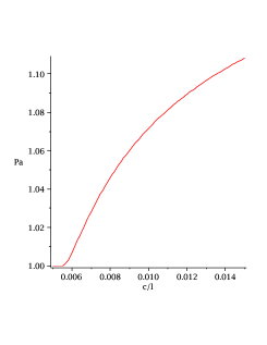
Figure 1: Price of anarchy for $c/\ell$ in the vicinity of $p^{+}=0.01$.

In this case, as $\gamma$ the fraction of agents investing in self-protection increases, the incentive to invest in self-protection decreases. In fact, it is less attractive for an agent to invest in self-protection, should others then decide to do so. As more agents invest, the expected benefit of following suit decreases since there is a reduction in the negative externalities which translates into a lower probability of loss. Hence there is a unique equilibrium point which is a Nash equilibrium. However, there is a wide range of parameters for which the Nash equilibrium will not be socially optimal because agents do not take into account the negative externalities they are creating in determining whether to invest or not. Indeed it is easily shown that at least for $c>p^{+}\ell$, the price of anarchy is strictly larger than one (see Figure 1).

Proposition 2

The fixed point equation (9,10,11,12) reduces to

$$h=\frac{h\ell}{c}\left(1-(1-p^{+})e^{-\lambda q^{+}h}\right)\mbox{ and, }1-\gamma=\frac{h\ell}{c}.$$

It has a unique solution. The price of anarchy is given by

$$P_{a}(c)=\sup_{\gamma}\frac{c}{\gamma c+h(\gamma)\ell},$$

where $h(\gamma)$ is the unique solution of

$$h=(1-\gamma)\left(1-(1-p^{+})e^{-\lambda q^{+}h}\right)$$

See Appendix 6.2 for a proof.

4.3 Case 2: Weak protection

We now consider Case 2 where $q^{+}=q^{-}$, so that $\gamma\mapsto c^{\gamma}$ is non-decreasing. The analysis of this case is described [10] (see Proposition 5). The situation is quite different from the results we derived for Case 1 above. In particular, we can have two Nash equilibria involving everyone or no one investing in security. When there are two Nash equilibria, the socially optimal solution is always for everyone to invest: each agent will find that the cost of investing in self-protection will be justified if it does not incur any negative externalities and society will be better off as well.

Proposition 3

We have $c^{0}<c^{1}$ and

• if $c<c^{0}$, then there is only one Nash equilibrium where every agent invest in self-protection;

• if $c>c^{1}$, then there is only one Nash equilibrium where no agent invest in self-protection;

• if $c^{0}<c<c^{1}$, then both Nash equilibria are possible.

The price of anarchy is given by:

$$P_{a}(c)=1\vee{\rm 11}(c^{0}<c)\frac{h(0)\ell}{c+h(1)\ell}.$$

If we take $p^{-}=0$, then we have $h(1)=0$ and $h(0)=h^{*}$ solution of $h^{*}=1-(1-p^{+})e^{-\lambda qh^{*}}$. So that we have

$$P_{a}(c)\sim\frac{h^{*}\ell}{c}.$$

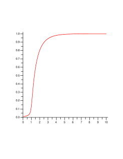
Figure 2: Price of anarchy: $h^{*}$ as a function of $\lambda q^{+}$, with $p^{+}=0.01$ and $p^{-}=0$.

Figure 2 shows the value of $h^{*}$ as a function of $\lambda q^{+}$. Note that typically $c=o(\ell)$ so that the price of anarchy can be substantially larger than one.

5 Discussion

We have shown that both situations with strong or weak protections exhibit externalities and that the equilibrium is not socially optimal: therefore, there is a market failure. However there are several important differences to understand between strong and weak protections before trying to resolve this market failure.

In case 1, the situation is similar to the free-rider problem which arises in the production of public goods. If all then agents invest in self-protection, then the general security level of the network is very high since the probability of loss is zero. But a self-interested agent would not continue to pay for self-protection since it incurs a cost $c$ for preventing only direct losses that have very low probabilities. When the general security level of the network is high, there is no incentive for investing in self-protection. This results in an under-protected network.

Note that in this case, if the cost for self-protection is not prohibitive, there is always a non-negligible fraction of the agents investing in self-protection. In case 2, the situation is quite different since no agent at all invests in self-protection. Even if a small fraction of agents does invest, and so raises the general level of security of the network, it is not sufficient for the benefit obtained by investing in self-protection for a new agent to be larger than the cost of self-protection.

These facts seem very relevant to the situation observed in the Internet, where under-investment in security solutions and security controls has long been considered an issue. Security managers typically face challenges in providing justification for security investments, and in 2003, the President’s National Strategy to Secure Cyberspace stated that government action is required where "market failures result in under-investment in cybersecurity" [15].

It shows the power of our basic model to note that these interesting and very relevant phenomena emerge from our analysis. Note also that these phenomena correspond to two extreme values of the parameter $q^{-}$, namely case 1 corresponds to $q^{-}=0$ and case 2 corresponds to $q^{-}=q^{+}$. Hence taking $p^{-}=0$ and fixing all other parameters, we have a family of models indexed by $q^{-}$, denoted simply $q$ in what follows, which varies ’continuously’ between the two cases.

Recall that $q$ is the probability of contagion when the agent invests in self-protection. If $q=0$, the agent is completely secure whereas for $q=q^{-}$, agents have the same probability of contagion whatever their choices to invest or not in self-protection. Hence $q$ can be interpreted as the inverse of the quality of the technology used for self-protection.

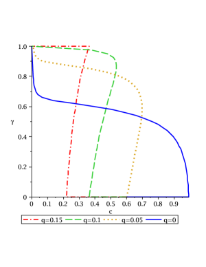
Figure 3: Adoption curves

First note that when $q=0$, the technology is ’perfect’ since there is no possible loss. We are in the situation of case 1 and we see that due to purely economic reasons, the technology is under-deployed in the network because people ’free-ride’ the benefit of the technology. Consider now the case of an arbitrary $q$. Figure 3 shows the adoption curves for different values of $q$. This curve shows the fraction of the population investing in security technology as a function of its cost (normalized by the loss). Other parameters are $p^{+}=0.01,q^{+}=0.5$ and $\lambda=10$.

We observe some counter-intuitive phenomena. First for a fixed price, increasing the quality of the security technology can lead to a decrease of its adoption in the population! Here is a qualitative interpretation of how this arises: when the technology is not very good, propagation of the epidemic is possible even if the agent uses the technology. Then agents have to pool their efforts in order to compensate for the weakness of the technology. In other words, a large number must invest in self-protection in order to have an acceptable level of security. But when the technology becomes better, then agents that did invest in it start to step down from the group of investors and choose to free-ride.

Second there is a barrier for choosing self-protection (except when $q=0$). Namely for a fixed $q$, we see that there is a range for the parameter $c$ (close to $c^{0}$) such that the population is ’trapped’ in state $N$ whereas for the same values of the parameters, the situation where a large fraction of the population is investing would be a sustainable equilibrium point. There is a possibility of tipping or cascading: inducing some agents to invest in self-protection will lead others to follow suit. The curves of Figure 3 allow us to quantify the minimal number of agents to induce in order to trigger a large cascade of adoption.

6 Appendix

6.1 Proof of Proposition 1

Recall that the RDE is given by:

$$Y\stackrel{{\scriptstyle d}}{{=}}1-(1-\phi)\prod_{k=1}^{N^{*}}(1-\theta_{k}Y_{k}),$$

where $N^{*}$ has distribution $P^{*}$, $\phi=DA^{S}+(1-D)A^{N}$, $\theta_{k}=DB^{S}_{k}+(1-D)B^{N}_{k}$ where $D$ is a Bernoulli r.v. with parameter $\gamma$, $Y$ and $Y_{k}$ are i.i.d. copies. Let $h=\mathbb{P}(Y=1)$, then we have

$$h = \mathbb{P}\left(D=1,(1-A^{S})\prod_{k=1}^{N^{*}}(1-B^{S}_{k}Y_{k})=0\right)$$

$$+\mathbb{P}\left(D=0,(1-A^{N})\prod_{k=1}^{N^{*}}(1-B^{N}_{k}Y_{k})=0\right)$$

$$= \gamma(1-\mathbb{P}(A^{S}=0))\mathbb{E}\left[\mathbb{P}(B^{S}_{k}Y_{k}=0)^{N^{*}}\right]$$

$$+(1-\gamma)(1-\mathbb{P}(A^{N}=0))\mathbb{E}\left[\mathbb{P}(B^{N}_{k}Y_{k}=0)^{N^{*}}\right],$$

and the first part of Proposition 1 follows.

We define:

$$f(x,\gamma) = 1-\gamma(1-p^{-})G_{N^{*}}(1-q^{-}x)$$

$$-(1-\gamma)(1-p^{+})G_{N^{*}}(1-q^{+}x),$$

so that $h$ is solution of the fixed point equation $h=f(h,\gamma)$. By taking the derivate of $f$ in $x$, we see that $x\mapsto f(x,\gamma)$ is a non-decreasing concave function. Note that $f(0,\gamma)=\gamma p^{-}+(1-\gamma)p^{+}\geq(1-\gamma)p^{+}$ and $f(1,\gamma)\leq 1$. So that for $\gamma<1$, there exists a unique solution to the fixed point equation $h=f(h,\gamma)$. If $\gamma=1$, we have $f(0,1)=p^{-}$ and $f(1,1)<1$. Then if $p^{-}=0$, the fixed point equation has a unique solution $h=0$ and if $p^{-}>0$, then $f(0,1)>0$ and the fixed point equation has still an unique solution.

We now prove that the function $\gamma\mapsto h(\gamma)$ is non-increasing. By taking the derivate of the function $\gamma\mapsto f(x,\gamma)$, we see that this function is non-increasing in $\gamma$ (while $x$ is fixed). Then for $u\leq v$, we get

$$f(h(u),u)=h(u)\geq f(h(u),v)\geq f(f(h(u),v),v)\geq h(v),$$

and the claimed monotonicity of $h$ follows.

6.2 Proof of Proposition 2

Recall that the fixed point equation for $h(\gamma)$ is:

$$h=(1-\gamma)\left(1-(1-p^{+})e^{-\lambda q^{+}h}\right).$$

Consider now that the cost $c$ and loss $\ell$ are random variables such that the function $t\mapsto\mathbb{P}(c/\ell\leq t)$ is continuous, then Equation (12) is

$$\gamma = \mathbb{P}\left(c\leq\ell\left(1-(1-p^{+})e^{-\lambda q^{+}h(\gamma)}\right)\right)$$

$$= \mathbb{P}\left(\frac{c}{\ell}\leq\frac{h(\gamma)}{1-\gamma}\right).$$

Since the function $h$ is non-increasing, we see that the right-hand side of the first line is a non-increasing function in $\gamma$, hence there exists a unique solution $\gamma^{*}$ to this fixed point equation. If we take a sequence of distributions such $c/\ell$ tends to a constant, we see that the solution $\gamma^{*}$ is such that

$$\frac{c}{\ell}=\frac{h(\gamma^{*})}{1-\gamma^{*}},$$

and the first part of Proposition 2 follows.

Note that we have $p^{N,\gamma}=h(\gamma)/(1-\gamma)$. So for a fixed $\gamma$, the average cost incured to the population is $\gamma c+(1-\gamma)p^{N,\gamma}\ell=\gamma c+h(\gamma)\ell$. Now for $\gamma=\gamma^{*}$, we have $h(\gamma^{*})\ell=(1-\gamma^{*})c$, so that the average cost is just $c$ and the last part of Proposition 2 follows.

References

- [1] D. Aldous and A. Bandyopadhyay. A survey of max-type recursive distributional equations. The Annals of Applied Probability, vol. 15, pp. 1047-1110, 2005.
- [2] D. Aldous and J.M. Steeele. The objective method: probabilistic combinatorial optimization and local weak convergence. Probability on discrete structures, Springer, vol. 110, pp. 1-72, 2004.
- [3] J. Bolot and M. Lelarge. A New Perspective on Internet Security using Insurance. Proc. IEEE Infocom 2008.
- [4] J. Bolot and M. Lelarge. Cyber-insurance as an incentive for IT security. Proc. Workshop Economics of Information Security (WEIS), 2008.
- [5] E.G. Coffman Jr., Z. Ge, V. Misra. Network resilience: exploring cascading failures within BGP. Proc. 40th Annual Allerton Conference on Communications, Computing and Control, October 2002.
- [6] R. Durrett Random graph Dynamics Cambridge U. Press, 2006.
- [7] A. Ganesh, L. Massoulie, D. Towsley. The effect of network topology on the spread of epidemics. Proc. IEEE Infocom 2005, Miami, FL, March 2005.
- [8] C. Gollier. The Economics of Risk and Time. MIT Press, 2004.
- [9] H. Kunreuther and G. Heal. Interdependent security: the case of identical agents. Journal of Risk and Uncertainty, 26(2):231–249, 2003.
- [10] M. Lelarge and J. Bolot. Network externalities and the deployment of security features and protocols in the Internet. Proc. ACM Sigmetrics, Annapolis, MD, Jun. 2008.
- [11] M. Lelarge and J. Bolot. A Local Mean Field Analysis of Security Investments in Networks. NetEcon’08, Seattle, Aug. 2008.
- [12] T. Moscibroda, Stefan Schmid and Roger Wattenhofer. When selfish meets evil: byzantine players in a virus inoculation game. PODC ’06: Proceedings of the twenty-fifth annual ACM symposium on Principles of distributed computing, 35–44, 2006.
- [13] N. Nisan, T. Roughgarden, E. Tardos and V.V. Vazirani (eds). Algorithmic game theory. Cambridge University Press, 2007.
- [14] M. Vojnovic and A. Ganesh. On the race of worms, alerts and patches. Proc. ACM Workshop on Rapid Malcode WORM05, Fairfax, VA, Nov. 2005.
- [15] White House. "National Strategy to Secure Cyberspace", 2003. Available at whitehouse.gov/pcipb.
- [16] C. Zou, W. Gong, D. Towsley. Code Red worm propagation modeling and analysis. Proc. 9th ACM Conf. Computer Comm. Security CCS’02., Washington, DC, Nov 2002.