A Parameterization Invariant Approach to the Statistical Estimation of the CKM Phase $\alpha$

Abstract:

In contrast to previous analyses, we demonstrate a Bayesian approach to the estimation of the CKM phase $\alpha$ that is invariant to parameterization. We also show that in addition to computing the marginal posterior in a Bayesian manner, the distribution must also be interpreted from a subjective Bayesian viewpoint. Doing so gives a very natural interpretation to the distribution.

We also comment on the effect of removing information about $\mathcal{B}^{00}$.

1 Introduction

A number of papers have been published recently that form a lively debate about the nature of inference in particle physics in general, and in the extraction of the CKM phase $\alpha$ from measured branching ratios and asymmetries in particular (see e.g. [1] and references therein for theoretical motivations and recent experimental results).

The first paper, Charles et al., [2], proposed several different parameterizations of the CKM phase $\alpha$ problem and showed, in their formulation, that different parameterizations resulted in different posterior marginal distributions for $\alpha$. These different distributions were held to be the result of using flat priors in the different parameterizations. The interpretation of $p(\alpha)$ in Charles et al. also claimed that it did not correctly identify the 8 known mirror solutions to the CKM phase $\alpha$ problem. Charles et al. also provided a simple 2-dimensional problem which they claimed showed similar features.

Charles et al. is a criticism of the approach taken by the UTfit collaboration [3], and Bona et al. replied in [4]. In this paper the emphasis is shifted from full distributions over $\alpha$ to 95% probability regions, which are shown to be very similar to the 95% confidence intervals given in Charles et al.. Bona et al. also note that the identification of the 8 modes in the 1-CL plot of Charles et al. is not robust to slight changes in the values of the observables, and that, in practice there is plenty of information regarding the hadronic amplitudes which can (and should) be used to remove some of the degeneracy.

Charles et al. replied in [5], criticizing the change of emphasis from $p(\alpha)$ to 95% probability intervals as being an admission that the approach of Bona et al. has significant dependence on the parametrization chosen. They also repeated their criticism that the Bayesian marginal posterior, $p(\alpha)$ does not show the expected 8-fold ambiguity.

A paper by Botella and Nebot [6] took another approach, noting that some parameterizations used in the analysis of the CKM phase $\alpha$ problem are inadequate if they go beyond the minimal Gronau and London assumptions [7]. In particular, the “modulus and argument” (MA) and “real and imaginary” (RI) parameterizations of Charles et al. were shown to not uniquely identify $\alpha$ in the parameterization, leading to the leaking of spurious information into $p(\alpha)$. Botella and Nebot identified which parameterizations do not suffer from this problem. They also, however, concentrated on probability regions, though they came tantalizingly close to giving the correct Bayesian interpretation of $p(\alpha)$ in their appendices C and E.

In this paper we will show how to perform a Bayesian analysis of the problem that results in the same $p(\alpha)$ for any parameterization. We also show how regarding $p(\alpha)$ as a Bayesian subjective distribution, i.e. one that describes our state of knowledge, allows it to be correctly interpreted in a straightforward manner – it is not sufficient just to use Bayes Theorem to perform computation, the result of that computation must also be interpreted from the Bayesian perspective.

We begin by reconsidering the simple 2-dimensional problem with mirror solutions of Charles et al.  as it is illustrative of some of the main points we wish to make.

2 Mirror Solutions in a Simple 2D Problem

The problem, from section VIII of [2], is presented as “a theory predicts the expressions of two observables X and Y as functions of the two parameters $\alpha$ and $\mu$”:

$$X = (\alpha+\mu)^{2}$$

$$Y = \mu^{2}\,,$$ (1)

where “an experiment has measured the observables from a Gaussian sample of events” with the results:

$$X = 1.00\pm 0.07$$

$$Y = 1.10\pm 0.07\,.$$ (2)

In terms of the assumed physics, only $\alpha$ is of interest.

It is important even at this early stage of the analysis to be clear regarding what is considered an “observable”, what is considered a “parameter”, and what is meant by saying that an observable has a distribution, or that a parameter has a distribution. Observables are expected to have values that vary with different experimental data sets, and saying that an observable has a distribution quantifies the uncertainty due to a particular data set. Saying that a parameter has a distribution is a Bayesian concept, indicating that there is actually a true, fixed, value, and that the distribution represents our state-of-knowledge regarding what that value might be.

This distinction is often somewhat artificial, however. Typically the quantities labeled as observables are not actually observed directly, instead they are themselves inferred from observed data. Different data sets will give different distributions over the observables and, consequently in the Bayesian framework, different distributions over the parameters. In equation 2, for example, the means and variances for $X$ and $Y$ are the summary results of a particular data set.

The standard approach to computing a joint Bayesian posterior distribution for $\alpha$ and $\mu$ is to use equations (1) and (2) to define a likelihood, and then to combine it with a prior, $p(\alpha,\mu)$, on $\alpha$, $\mu$, giving

$$p_{\alpha,\mu}(\alpha,\mu|d)\propto\frac{1}{2\pi\sigma_{X}\sigma_{Y}}\exp\left(-\frac{[(\alpha+\mu)^{2}-\bar{X}]^{2}}{2\sigma_{X}^{2}}-\frac{[\mu^{2}-\bar{Y}]^{2}}{2\sigma_{Y}^{2}}\right)p(\alpha,\mu)$$ (3)

where $d$ denotes the experimental data and $\bar{X}$, $\bar{Y}$, $\sigma_{X}$ and $\sigma_{Y}$ are derived by considering the full expression for the likelihood over the individual measurements. They are all functions of $d$ .

This formulation is subject to the standard criticism that different parameterizations require different priors – if, for example, we were to parameterize the problem by $\alpha$, $\mu^{\prime}$ where $\mu^{\prime}=\mu^{2}$, then clearly flat priors on $\mu$ and $\mu^{\prime}$ will result in different posterior distributions [8].

The discussion of observables and parameters above motivates an alternative Bayesian analysis, one that results in a posterior distribution that is invariant to the parameterization chosen. In this analysis we first use the observed data to obtain a posterior distribution over $X$ and $Y$. This requires a prior on the observables, and yields

$$p_{X,Y}(x,y|d)\propto\frac{1}{2\pi\sigma_{X}\sigma_{Y}}\exp\left(-\frac{(x-\bar{X})^{2}}{2\sigma_{X}^{2}}-\frac{-(y-\bar{Y})^{2}}{2\sigma_{Y}^{2}}\right)p(x,y)\,.$$ (4)

Placing priors in the space of observables is reasonable: it is here that the experimenter will typically have good prior knowledge – prior knowledge that determined the design of the experiment.

The physical parameters of interest, $\alpha$, $\mu$ are related to $X$, $Y$ by the deterministic relationships in equation (1). The distribution $p_{\alpha,\mu}(\alpha,\mu|d)$ is thus computed by the change of variables rule. When the posterior for $\alpha$, $\mu$ is computed in this way, the general result in Appendix A can be used to show that the resulting posterior marginal distribution, $p_{\alpha}(\alpha|d)$ is invariant with respect to the chosen parameterization of the other variables (in this case, $\mu$).

Changing variables gives

$$p_{\alpha,\mu}(\alpha,\mu|d)\propto p_{X,Y}(x(\alpha,\mu),y(\alpha,\mu)|d)\left|\frac{\partial(X,Y)}{\partial(\alpha,\mu)}\right|$$ (5)

resulting in

$$p_{\alpha,\mu}(\alpha,\mu|d)\propto\frac{1}{2\pi\sigma_{X}\sigma_{Y}}\exp\left(-\frac{[(\alpha+\mu)^{2}-\bar{X}]^{2}}{2\sigma_{X}^{2}}-\frac{[\mu^{2}-\bar{Y}]^{2}}{2\sigma_{Y}^{2}}\right)|\mu(\alpha+\mu)|$$ (6)

on the assumption of a flat prior $p(x,y)$, and where the factor of 4 is removed because of the multiple solutions. This is plotted in figure 1.

Comparing equation (6) with equation (3) it is clear that this transformation of variables formulation is equivalent to using the prior

$$p(\alpha,\mu)\propto|\mu(\alpha+\mu)|.$$

In this problem it is straightforward to show that the Jeffrey’s prior [9], given by $\sqrt{|I(\alpha,\mu)|}$ where $I()$ is the Fisher Information matrix, is also proportional to $|\mu(\alpha+\mu)|$. The Jeffrey’s prior is the prior that is invariant to transformation of the variables. Thus, computing a posterior $p_{X,Y}(x,y|d)$ using a uniform prior on $X$ and $Y$ followed by a transformation of variables to give $p_{\alpha,\mu}(\alpha,\mu|d)$ is equivalent o using a Jeffrey’s prior on $\alpha$, $\mu$.

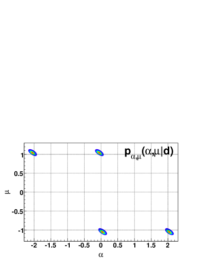
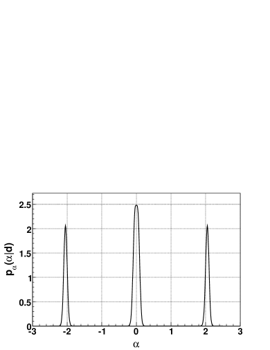
Figure 1: Left : The posterior distribution of $\mu,\alpha$; Right : the marginal distribution $p_{\alpha}(\alpha|\mbox{\boldmath$d$})$.

While figure 1 (left) looks very similar in projection to figure 5 in [2], note, however, that the modes of $p_{\alpha,\mu}(\alpha,\mu)$ are not located at the values of $\alpha$ that were found by substituting the mean values $\bar{X}$ and $\bar{Y}$ into equations (1). They are shifted because of the presence of the term $|\mu(\alpha+\mu)|$ in the expression for $P_{\alpha,\mu}(\alpha,\mu)$ in equation (6), coming from the determinant of the Jacobian of the transformation from $X,Y$ to $\alpha,\mu$. In this case the displacement of the modes is small; it is not visible in figure 1. This need not be the case in general, and indeed is not the case for the CKM phase $\alpha$ problem. See section 3.

The simplest way to form the marginal distribution $p(\alpha)$ is to generate samples from the distributions of $X$ and $Y$, to transform these samples into samples of $\alpha$ and $\mu$, and then to plot a histogram of the samples of $\alpha$ [10]. In this case we generate samples $x_{i}\leftarrow\mathcal{N}(1.00,0.07)$ and $y_{i}\leftarrow\mathcal{N}(1.10,0.07)$, $i=1\ldots N$ for some suitably large $N$, and from each pair $(x_{i},y_{i})$ we find the four solutions for $(\alpha_{i},\mu_{i})$, namely

$$\alpha_{i} = \epsilon_{x}\sqrt{x_{i}}-\epsilon_{y}\sqrt{y_{i}}$$

$$\mu_{i} = \epsilon_{y}\sqrt{y_{i}}$$ (7)

where $\epsilon_{x}=\pm 1$, $\epsilon_{y}=\pm 1$ and each of the four $(\alpha_{i},\mu_{i})$ pairs is given weight 1/4.

In the right panel of figure 1 we plot the marginal distribution $p_{\alpha}(\alpha|\mbox{\boldmath$d$})$, which is very similar to figure 6 (bottom) from Charles et al.. In their discussion of this figure, Charles et al. state that “if $\alpha$ and $\mu$ are fundamental physics parameters, Nature can only accommodate a single pair of values”, and criticize the Bayesian approach by saying that the marginal $p_{\alpha}(\alpha|\mbox{\boldmath$d$})$ only has 3 peaks, with the peak at zero being higher than the other two. This is an incorrect interpretation of the distribution. This distribution is in fact exactly right when interpreted as a Bayesian subjective distribution, as representing our state of knowledge. Nature has chosen one of the four modes visible in the joint distribution $p_{\alpha,\mu}(\alpha,\mu)$. We do not know which one. On the basis of our knowledge, there are two chances out of four that Nature has chosen $\alpha\approx 0$, so our state of knowledge is exactly that $\alpha\approx 0$ is twice as likely as $\alpha\approx-2$ or $\alpha\approx 2$. This is precisely what is shown by the distribution in the right panel of figure 1, where the central mode has twice the area of each of the other two modes.

This simple problem has illustrated two of the key points we wish to make, namely that the posterior distribution must be interpreted in a subjective Bayesian manner, and that the posterior distribution in this type of problem can be found by putting priors in the space of observables, and then using the transformation of variables rule to compute the distribution over the parameters derived from the observables. The simple problem is not rich enough to clearly demonstrate that this approach also leads to posterior distributions for $\alpha$ which are independent of the parameterization chosen. To do this, we turn now to the full CKM phase $\alpha$ problem.

3 Extracting the CKM Phase $\alpha$

There are six observable parameters involved in the CKM Phase $\alpha$ problem, three CP averaged branching fractions, $\mathcal{B}^{+-}$, $\mathcal{B}^{+0}$, $\mathcal{B}^{00}$, the direct CP asymmetries $C^{+-}$and $C^{00}$, and the $B^{0}\bar{B}^{0}$ mixing-induced CP asymmetry, $S^{+-}$. These have been recently measured by the B-factory experiments BaBar and Belle [1, 11].

The general formula for the branching ratio of a 2-body decay of a meson B can be found in [12] (eqs. 38.16 and 38.17). Specializing to a final state of light mesons, and averaging over CP-eigenstate yields:

$${\cal B}^{ij} = \frac{\tau_{B}^{i+j}}{16\pi M_{B}\hbar}\frac{|A^{ij}|^{2}+|\bar{A}^{ij}|^{2}}{2}$$

$$C^{ij} = \frac{|A^{ij}|^{2}-|\bar{A}^{ij}|^{2}}{|A^{ij}|^{2}+|\bar{A}^{ij}|^{2}}$$

$$S^{+-} = \frac{2Im(\bar{A}^{+-}A^{+-*})}{|A^{+-}|^{2}+|\bar{A}^{+-}|^{2}}\,.$$

The decay amplitudes can be parameterized in a number of ways. Here we will consider three parameterizations, the Pivk-LeDiberder (PLD) and Explicit Solution (ES) parameterizations considered in Charles et al. and the so-called 1i parameterization from Botella and Nebot. These vary in how they parameterize $A^{ij}$ and $\bar{A}^{ij}$, but all include $\alpha$ explicitly as one of the parameters. Details of the parameterizations are given in appendix B.

Denote the parameterizations as $(\alpha,\phi_{PLD})$, $(\alpha,\phi_{ES})$ and $(\alpha,\phi_{1i})$, where $\phi_{PLD}$ denotes the other five parameters of the PLD parameterization, and similarly for $\phi_{ES}$ and $\phi_{1i}$. Denote by $O$ the set of six observables, $\mathcal{B}^{+-}$, $\mathcal{B}^{00}$, $\mathcal{B}^{+0}$, $C^{+-}$, $C^{00}$ and $S^{+-}$. Then we have

$$O = f(\alpha,\phi_{PLD})$$

$$= g(\alpha,\phi_{ES})$$

$$= h(\alpha,\phi_{1i})\ ,$$

where the functional forms of $f()$, $g()$ and $h()$ can be derived from the parameterizations given in Appendix B. Table 1 gives the values for the observables and their uncertainty that are used in this work . Using a uniform prior in the space of observables, these define a multivariate Gaussian posterior, $p(\mbox{\boldmath$O$}|d)$ where $d$ is the experimental data.

Observable	$\mathcal{B}^{+-}$	$\mathcal{B}^{+0}$	$\mathcal{B}^{00}$
Mean$\pm$std	$(5.1\pm 0.4)\times 10^{-6}$	$(5.5\pm 0.6)\times 10^{-6}$	$(1.45\pm 0.29)\times 10^{-6}$
Observable	$C^{+-}$	$C^{00}$	$S^{+-}$
Mean$\pm$std	$-0.37\pm 0.10$	$-0.28\pm 0.40$	$-0.50\pm 0.12$

Table 1: World average values for the observables, from [2].

Using the change-of-variables formulation gives

$$p_{PLD}(\alpha,\phi_{PLD})=p(f(\alpha,\phi_{PLD})|d)|J_{f}|$$

and the marginal distribution for $\alpha$ is given by

$$p_{PLD}(\alpha)=\int_{\phi_{PLD}}p(f(\alpha,\phi_{PLD})|d)|J_{f}|d\phi_{PLD}.$$ (8)

Similarly

$$p_{1i}(\alpha)=\int_{\phi_{1i}}p(h(\alpha,\phi_{1i})|d)|J_{h}|d\phi_{1i}.$$ (9)

In appendix A we show that under reasonable conditions these marginal distributions are identical, i.e. that the marginal posterior distribution for $\alpha$ is independent of the chosen parameterization. This should not be surprising – the same information on the same observables gives the same information about the same physical parameter.

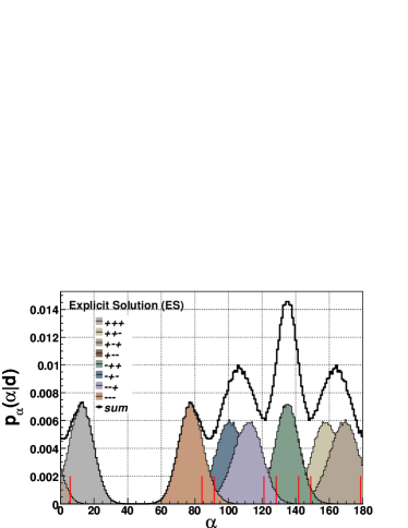
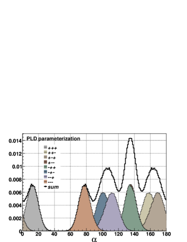
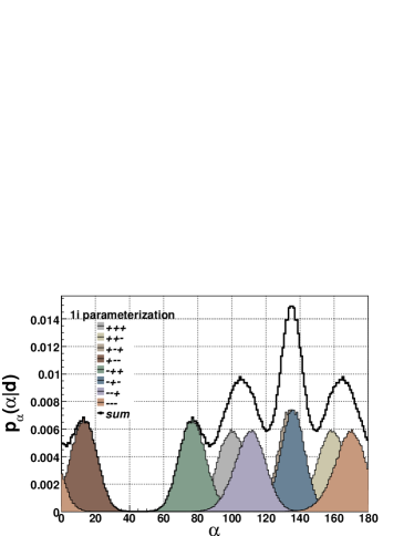
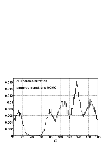
Figure 2: The first three plots show the marginal posterior distributions for $\alpha$ under the PLD, ES and 1i parameterizations generated by inverting the systems. The short vertical red lines on the top left plot indicate the central values obtained by [2]. Legends indicate the tuple of signs corresponding to each mode. The final plot is of samples generated from the PLD parameterization using the tempered transitions MCMC scheme. Binning in $\alpha$ is identical for all figures. In the first three plots, a sample of 100000 sets of observables is drawn, and the choices of signs, as indicated by the legends, allows each mode to be determined separately. As a result, the sum histograms have 800000 non independent entries. The fourth histogram is of size 100000.

In figure 2 we plot histograms representing the three marginal posterior distributions. The samples were generated by sampling the observables and inverting the systems . As expected, the three histograms are essentially identical. We also show a histogram of samples generated using the PLD parameterization and a Markov chain Monte Carlo algorithm [13]. As expected, the histogram is the same as the others. It is included to demonstrate that our approach is not restricted to cases where the system can be inverted. Care must be taken in choosing the MCMC scheme, as the distribution is strongly multimodal. We used the simulated tempering scheme of [14] which successfully sampled the 8 modes of the distribution.

If we consider the modulus-and-argument (MA) parameterization [3, equation 4], we will not, however recover the same distribution for $\alpha$. The determinant of the Jacobian for the MA system is identically zero for $\alpha=0$, and this results in a spurious zero in probability at $\alpha=0$, the remainder of the distribution being identical to our figure 2. This adds to the discussion in [6] that the MA parameterization, by going beyond the minimal Gronau and London assumptions, is unsuited to the analysis of this problem.

The histograms generated by inverting the systems are clearly composed of 8 modes, one for each of the 8 solutions. (There are two modes that overlap almost totally around $\alpha\approx 140^{\circ}$.) By construction, each of these modes has equal probability mass (=1/8), even though they are different shapes; the heights and widths vary, but the area beneath each mode is the same. Each possible solution for $\alpha$ has different uncertainty (due to the complex relationship between $\alpha$ and the observables), but each mode has equal probability to be the one chosen by Nature.

The final marginal distribution is the sum of these 8 modes, which is plotted as the dotted line. This shows a large peak around $\alpha=140^{\circ}$ and a number of smaller peaks. Again, this distribution correctly describes our state of knowledge – there are 2 of the 8 modes near $\alpha=140^{\circ}$ and, because we don’t know which mode Nature has chosen, there are thus 2 chances out of 8 that $\alpha\approx 140^{\circ}$. There is only 1 chance out of 8 that $\alpha\approx 80^{\circ}$, so the peak there has half the area of the peak at $\alpha=140^{\circ}$. This accurately represents our state of knowledge about $\alpha$.

Also shown on figure 2 are short vertical lines marking the values of $\alpha$ that are found when the mean values for the observables are transformed into the different parameterizations. Again, it comes as no great surprise that the mean of the distribution of the inputs is not transformed to the mean of the distribution of the output, especially when the uncertainty on some of the variables is of the same order as the value itself, and the system of equations is highly nonlinear. This also naturally explains why there is still finite probability density that $\alpha=0/180^{\circ}$.

As the methodology presented in this work relies on the one-to-one relationship (up to discrete ambiguities) between the observables {$\mathcal{B}^{+-}$, $\mathcal{B}^{+0}$, $\mathcal{B}^{00}$, $C^{+-}$, $C^{00}$, $S^{+-}$} and the underlying isospin amplitude representation, the analysis of the case when $\mathcal{B}^{00}$and $C^{00}$are not measured is not in general possible, once the system has been inverted. For instance, although the PLD representation presents the very appealing feature that $\alpha$ appears in the system (15) only in the expressions for $\mathcal{B}^{00}$and $C^{00}$, and therefore cannot be determined when the latter are not measured, this feature is not obvious anymore in the inverted system (16). This is equivalent to the fact, already mentioned in Botella and Nebot (section C.1), that {$\mathcal{B}^{00}$, $C^{00}$} are algebraically constrained by any set of measurements {$\mathcal{B}^{+-}$, $\mathcal{B}^{+0}$, $C^{+-}$, $S^{+-}$} and the assumption of isospin symmetry. As noted by Botella and Nebot, sampling $C^{00}$ uniformly between $-1$ and $+1$, and $\mathcal{B}^{00}$ between $0$ and $B_{max}$, results in a distribution that is much flatter than those shown in figure 2. This distribution does not, however, become flat as $B_{max}\rightarrow\infty$, because ultimately the shape of the underlying single mode distributions will be driven by the algebraic constraints from the isospin assumption and by the error propagation from the measured observables. As an illustration, we show in figure 3 the result of the ‘1i’ parameterization for $B_{max}=20\mathcal{B}^{00}$. Increasing the upper bound on $\mathcal{B}^{00}$ will not change the final distribution, but will result in more samples being thrown away as incompatible with the constraints on the system. Figure 3 (right) shows a histogram of the samples of $\mathcal{B}^{00}$ and $C^{00}$ that were retained. It shows the probabilistic constraints on $\mathcal{B}^{00}$ and $C^{00}$ due to the observations and the assumption of isospin symmetry.

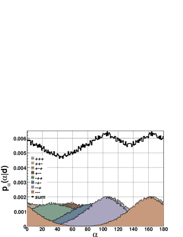
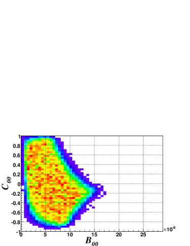
Figure 3: Left: Posterior distribution for the ’1i’ parameterization when $C^{00}$and $\mathcal{B}^{00}$are uniformly sampled in [-1, +1] and [0, 20$\mathcal{B}^{00}$], respectively. Sampling is identical to figure 2. Right: Joint distribution of $\mathcal{B}^{00}$ and $C^{00}$ implied by the observations and the assumption of isospin symmetry.

4 Conclusions

In the debate concerning the analysis of the CKM phase $\alpha$ problem we have contributed two important points. The first is a formulation of the problem that is invariant to the choice of parameterization. The second is the correct interpretation of the posterior marginal distribution for $\alpha$ as a representation of our state of knowledge.

In the CKM Phase $\alpha$ problem the relationships between the parameters of the model and the observables is deterministic. In this case the appropriate statistical technique to find the distribution over the model parameters is that of the transformation-of-variables. This gives us a distribution over the model parameters that summarizes our state of knowledge. It does not, and cannot, tell us if our model is true or false. We have no way of knowing the actual mechanisms of the external universe. We can only generate models of the universe and use data to cast light on these models. However “true” we may think our models are today, better models will certainly be developed tomorrow. The scientific method is composed of the cycle of model formulation, testing against observations, and model revision and development. Bayesian statistics provides many tools to facilitate this process.

Appendix A Reparameterization invariance of the marginal posterior pdf over $\alpha$ 

We consider a system of $N$ random variables $X_{i}$ ($i=1...N$), which are related to a set of $N$ observables ${\cal O}_{i}$ as ${{\cal O}_{i}}=f_{i}(\mathbf{X})$. We also assume that it is possible to reparameterize the variables $X_{i}$ into a set $Y_{i}$ so that $X_{1}=Y_{1}=\alpha$, $Y_{i}=\phi_{i}(\mathbf{X})$, and ${\cal O}_{i}=g_{i}(\mathbf{Y})$. Within the Bayesian framework, we consider a dataset ${d}$ used to estimate the observables, which yields the posterior pdf $p_{\mathbf{\cal O}}(\mathbf{o}|d)$. Under the further hypothesis that $f$, $g$ and $\phi$ are invertible, we can write the marginal posterior on $\alpha$ using the parameterization $Y$ as:

$$p^{\mathbf{Y}}_{\alpha}(\alpha|{d}) = \int...\int p_{\mathbf{\cal O}}(\mathbf{o}|d)|J_{g}|dy_{2}...dy_{N}\,\mbox{as}\,p_{\mathbf{X}}(\mathbf{x}|{d})=p_{\mathbf{\cal O}}(\mathbf{o}|d)|J_{g}|$$ (10)

$$= \int...\int p_{\mathbf{\cal O}}(\mathbf{o}|d)|J_{g}||J_{\phi}|dx_{2}...dx_{N}$$ (11)

$$= \int...\int p_{\mathbf{\cal O}}(\mathbf{o}|d)|J_{f}|dx_{2}...dx_{N}$$ (12)

$$= p^{\mathbf{X}}_{\alpha}(\alpha|{d})\,\mbox{as }\,p_{\mathbf{Y}}(\mathbf{y}|{d})=p_{\mathbf{\cal O}}(\mathbf{o}|d)|J_{f}|,$$ (13)

proving that the marginal posterior on $\alpha$ is parameterization invariant. Thus, if a Bayesian analysis has been performed on the dataset ${d}$ so that the posterior pdf on the observables is known, the marginal posterior on $\alpha$ obtained by the change of variables $Y_{i}=\phi_{i}(\mathbf{X})$ is invariant under reparameterization of the $N-1$ marginalized variables $X_{i}$, $i=2\ldots N$.

Appendix B Parameterizing the CKM Phase $\alpha$ Problem

We give details here of the three parameterizations, the Pivk-LeDiberder (PLD), the Explicit Solution (ES) and the 1i parameterizations.

B.1 The Pivk-LeDiberder Parameterization

PLD introduces six parameters, $\alpha,\alpha_{eff},\mu,a,\bar{a},\Delta$, via

$$A^{+-}=\mu a\ \ \bar{A}^{+-}=\mu\bar{a}e^{2i\alpha_{eff}}$$ ,

$$A^{+0}=\mu e^{i(\Delta-\alpha)} \bar{A}^{+0}=\mu e^{i(\Delta+\alpha)}$$ , (14)

$$A^{00}=\mu e^{i(\Delta-\alpha)}\left(1-\frac{a}{\sqrt{2}}e^{-i(\Delta-\alpha)}\right) \bar{A}^{00}=\mu e^{i(\Delta+\alpha)}\left(1-\frac{\bar{a}}{\sqrt{2}}e^{-i(\Delta+\alpha-2\alpha_{eff})}\right)$$ ,

which results in

$$\mathcal{B}^{+-} = C\frac{\tau_{B^{0}}}{2}\mu^{2}(a^{2}+\bar{a}^{2})$$

$$\mathcal{B}^{00} = C\frac{\tau_{B^{0}}}{2}\mu^{2}\left(2+\frac{a^{2}+\bar{a}^{2}}{2}-\sqrt{2}(a\cos{(\Delta-\alpha)}+\bar{a}\cos{(\Delta+\alpha-2\alpha_{eff})})\right)$$

$$\mathcal{B}^{+0} = C\tau_{B^{+}}\mu^{2}$$

$$C^{+-} = \frac{a^{2}-\bar{a}^{2}}{a^{2}+\bar{a}^{2}}$$ (15)

$$C^{00} = \frac{\frac{a^{2}-\bar{a}^{2}}{2}-\sqrt{2}(a\cos{(\Delta-\alpha)}-\bar{a}\cos{(\Delta+\alpha-2\alpha_{eff})})}{2+\frac{a^{2}+\bar{a}^{2}}{2}-\sqrt{2}(a\cos{(\Delta-\alpha)}+\bar{a}\cos{(\Delta+\alpha-2\alpha_{eff})})}$$

$$S^{+-} = 2\frac{a\bar{a}}{a^{2}+\bar{a}^{2}}\sin{2\alpha_{eff}}$$

where $C=(16\pi M_{B}\hbar)^{-1}$. This system can be solved to give

$$\mu^{2} = \frac{\mathcal{B}^{+0}}{C\tau_{B^{+}}}$$

$$a^{2} = K(1+C^{+-})$$

$$\bar{a}^{2} = K(1-C^{+-})$$

$$\sin{2\alpha_{eff}} = \frac{S^{+-}}{\sqrt{1-(C^{+-})^{2}}}\equiv\sin{s}$$ (16)

$$\cos{(\Delta-\alpha)} = \frac{(1+C^{+-})K-2K\frac{\mathcal{B}^{00}}{\mathcal{B}^{+-}}(1+C^{00})+2}{2\sqrt{2K(1+C^{+-})}}\equiv\cos{t}$$

$$\cos{(\Delta+\alpha-2\alpha_{eff})} = \frac{(1-C^{+-})K-2K\frac{\mathcal{B}^{00}}{\mathcal{B}^{+-}}(1-C^{00})+2}{2\sqrt{2K(1-C^{+-})}}\equiv\cos{u}$$

where we define $\displaystyle{K=\frac{\mathcal{B}^{+-}}{\mathcal{B}^{+0}}\frac{\tau_{B^{+}}}{\tau_{B^{0}}}}$, and $s,t$ and $u$ as in the final three equations. The fourth equation yields $2\alpha_{eff}=s$ or $2\alpha_{eff}=\pi-s$. The final two equations yield $\Delta+\alpha=\epsilon t+s$ or $\Delta+\alpha=\epsilon t+\pi-s$ and $\Delta-\alpha=\epsilon^{\prime}u$ or $\Delta+\alpha=\epsilon t+\pi-s$, respectively, where $\epsilon,\epsilon^{\prime}=\pm 1$. Finally, we obtain $\alpha=\epsilon t+\epsilon^{\prime}u+s$ or $\alpha=\epsilon t+\epsilon^{\prime}u+\pi-s$ as the 8 solutions corresponding to each set of values of the observables.

B.2 The Explicit Solution Parameterization

The Explicit Solution (ES) parameterization [17] begins with the same parameters as the PLD parameterization, and then defines

$$c = \cos(\phi),\,\phi=\alpha-\Delta$$

$$\bar{c} = \cos(\bar{\phi}),\,\bar{\phi}=\alpha+\Delta-2\alpha_{eff}$$

and also $s=\sin(\alpha)$, $\bar{s}=\sin(\bar{\phi})$. Using the identity $2\alpha=2\alpha_{eff}+\phi+\bar{\phi}$ allows the following solution to be derived.

$$\tan\alpha = \frac{\sin(2\alpha_{eff})\bar{c}+\cos(2\alpha_{eff})\bar{s}+s}{\cos(2\alpha_{eff})\bar{c}-\sin(2\alpha_{eff})\bar{s}+c}$$

$$\sin(2\alpha_{eff}) = \frac{S^{+-}}{\sqrt{1-C^{+-}{}^{2}}}$$

$$\cos(2\alpha_{eff}) = \pm\sqrt{1-\sin^{2}(2\alpha_{eff})}$$

$$c = \sqrt{\frac{\tau_{B^{+}}}{\tau_{B^{0}}}}\frac{\frac{\tau_{B^{0}}}{\tau_{B^{+}}}\mathcal{B}^{+0}+\mathcal{B}^{+-}(1+C^{+-})/2-\mathcal{B}^{00}(1+C^{00})}{\sqrt{2\mathcal{B}^{+-}\mathcal{B}^{+0}(1+C^{+-})}}$$

$$\bar{c} = \sqrt{\frac{\tau_{B^{+}}}{\tau_{B^{0}}}}\frac{\frac{\tau_{B^{0}}}{\tau_{B^{+}}}\mathcal{B}^{+0}+\mathcal{B}^{+-}(1-C^{+-})/2-\mathcal{B}^{00}(1-C^{00})}{\sqrt{2\mathcal{B}^{+-}\mathcal{B}^{+0}(1-C^{+-})}}$$

$$s = \pm\sqrt{1-c^{2}}$$

$$\bar{s} = \pm\sqrt{1-\bar{c}^{2}}$$ (17)

where the 8 solutions in the range $[0,\pi]$ are apparent from the three arbitrary signs.

B.3 The 1i Parameterization

Botella and Nebot introduce the following parameterization

$$A^{+-} = e^{-i\alpha}T_{3/2}(T+iP)$$

$$\sqrt{2}A^{+0} = e^{-i\alpha}T_{3/2}$$

$$\bar{A}^{+-} = e^{+i\alpha}T_{3/2}(T-iP)$$

$$\sqrt{2}A^{00} = e^{-i\alpha}T_{3/2}(1-T-iP)$$

$$\sqrt{2}\bar{A}^{+0} = e^{+i\alpha}T_{3/2}$$

$$\sqrt{2}\bar{A}^{00} = e^{+i\alpha}T_{3/2}(1-T-iP)$$

and writing $T$ and $P$ in terms of real and imaginary parts allows the system of equations for the observables to be inverted in terms of $\alpha$, $T_{3/2}$, $T_{r}$, $T_{i}$, $P_{r}$, $P_{i}$, in the following way :

$$T = \sqrt{\frac{2\mathcal{B}^{+0}}{\tau_{B^{+}}C}}$$

$$T_{r} = \frac{2\,\mathcal{B}^{+0}\,\tau_{B^{0}}+\left(\mathcal{B}^{+-}-2\,\mathcal{B}^{00}\right)\,\tau_{B^{+}}}{4\,\mathcal{B}^{+0}\,\tau_{B^{0}}}$$

$$P_{i} = \frac{\left(2\,\mathcal{B}^{00}\,C^{00}-\mathcal{B}^{+-}\,C^{+-}\right)\,\tau_{B^{+}}}{4\,\mathcal{B}^{+0}\,\tau_{B^{0}}}$$

$$(T_{i}+P_{r})^{2} = \frac{\mathcal{B}^{+-}\tau_{B^{+}}}{2\mathcal{B}^{+0}\tau_{B^{0}}(1+C^{+-})}-(T_{r}-P_{i})^{2}$$

$$(T_{i}-P_{r})^{2} = \frac{\mathcal{B}^{+-}\tau_{B^{+}}}{2\mathcal{B}^{+0}\tau_{B^{0}}(1-C^{+-})}-(T_{r}+P_{i})^{2}$$

$$\alpha = \arctan\left(\pm\frac{\sqrt{b^{2}+a^{2}-c^{2}}+a}{c-b}\right)$$

with $a=(T_{i}^{2}-P_{i}^{2}+T_{r}^{2}-P_{r}^{2}),\,b=2P_{i}T_{i}+2P_{r}T_{r},\,c=S^{+-}\mathcal{B}^{+-}\tau_{B^{+}}/(2\tau_{B^{0}}\mathcal{B}^{+0})$.

References

- [1] B. Aubert et al. [BABAR Collaboration], Phys. Rev. D 76 (2007) 091102 \arXivid0707.2798
- [2] J. Charles, A. Höcker, H. Lacker. F.R. Le Diberder and S.T’Jampens, hep-ph/0607246, 22 July 2006
- [3] M. Bona et al. [UTfit Collaboration], J. High Energy Phys. 07 (2005) 028
- [4] M. Bona et al. [UTfit Collaboration], Phys. Rev. D 76 (2007) 014015 hep-ph/0701204
- [5] J. Charles, A. Höcker, H. Lacker. F.R. Le Diberder and S.T’Jampens, hep-ph/0703073, March 2007
- [6] F.J. Botella and M. Nebot, \arXivid0704.0174, April 2007
- [7] M. Gronau and D. London, Phys. Rev. Lett. 65 (1990) 3381-3384
- [8] H. Prosper, “Bayesian Analysis”. Proceedings of the Workshop on Confidence Limits, CERN, 17-18 January 2000. hep-ph/0006356, June 2000
- [9] R.E. Kass and L. Wasserman, JASA 91, 435, pp 1343-1370, (1996)
- [10] A.F.M. Smith and A.E. Gelfand, The American Statistician, 46, 2, pp 84-88, (1992)
- [11] H. Ishino et al. [Belle Collaboration], Phys. Rev. Lett. 98 (2007) 211801 hep-ex/0608035
- [12] W.-M. Yao et al., J. Phys. G 33 (2006) 1
- [13] C.P. Robert and G. Casella, Monte Carlo Statistical Methods, Springer, 2nd edition, (2004)
- [14] R. Neal, Statistics and Computing, 6, 4, pp 353-366, (1996)
- [15] J. Charles et al. [CKMfitter Group], Eur. Phys. J. C 41 (2005) 1 hep-ph/0406184
- [16] D.S. Sivia with J. Skilling, Data Analysis: A Bayesian Tutorial, 2nd edition, Oxford University Press, 2006
- [17] M. Pivk and F.R. Le Diberder, Eur. Phys. J. C 39 (2005) 397-409 hep-ph/0406263