Finite-size scaling of the entanglement entropy of the quantum Ising chain with homogeneous, periodically modulated and random couplings

Abstract

Using free-fermionic techniques we study the entanglement entropy of a block of contiguous spins in a large finite quantum Ising chain in a transverse field, with couplings of different types: homogeneous, periodically modulated and random. We carry out a systematic study of finite-size effects at the quantum critical point, and evaluate subleading corrections both for open and for periodic boundary conditions. For a block corresponding to a half of a finite chain, the position of the maximum of the entropy as a function of the control parameter (e.g. the transverse field) can define the effective critical point in the finite sample. On the basis of homogeneous chains, we demonstrate that the scaling behavior of the entropy near the quantum phase transition is in agreement with the universality hypothesis, and calculate the shift of the effective critical point, which has different scaling behaviors for open and for periodic boundary conditions.

1 Introduction

Entanglement describes nonlocal quantum correlations, and is one of the characteristic peculiar features of quantum mechanics. Motivated by recent studies showing intimate connections between entanglement and quantum phase transitions [1, 2], the understanding of the degree of entanglement in quantum many-body systems has prompted an enormous effort at the interface between condensed matter physics, quantum information theory and quantum field theory [3].

A fundamental question in this research field is concerned with the scaling of the entropy quantifying the degree of entanglement between a spatially confined region and its complement in a quantum many-body system. Suppose a system, combined by two subsystems $\mathcal{A}$ and $\mathcal{B}$, is in a pure quantum state $|\psi\rangle$, with density matrix $\rho=|\psi\rangle\langle\psi|$. The entanglement entropy is just the von Neumann entropy of either subsystem given by

$$S_{\cal A}=-\Tr(\rho_{\cal A}\log_{2}\rho_{\cal A})=-\Tr(\rho_{\cal B}\log_{2}\rho_{\cal B})=S_{\cal B},$$ (1)

where the reduced density matrix for $\cal A$ is constructed by tracing over the degrees of freedom in $\cal B$, given by $\rho_{\cal A}=\Tr_{\cal B}\rho$. Analogously, $\rho_{\cal B}=\Tr_{\cal A}\rho$. In order to explore the behavior of quantum entanglement at different length scales, one is particularly interested in how the entanglement entropy depends on the linear size $\ell$ of the subsystem considered. An early conjectured scaling law relates the entanglement entropy to the surface area $\ell^{d-1}$, not the volume, of the region in a $d$-dimensional system [4]. This area law of entropy scaling has been established for gapped quantum many-body systems where the correlation length is finite. In one-dimensional (1D) systems, the entanglement behavior changes drastically at a quantum phase transition where the absence of gaps leads to long range correlations and results in a logarithmically diverging entanglement entropy as the system size $L$ goes to infinity, i.e. $S_{\mathcal{A}}\sim\log_{2}\ell$ for $L\to\infty$ [5, 6, 7, 8]. This connection between entanglement entropy and quantum phase transitions is however lost in quantum systems in higher dimensions [9, 10, 11, 12, 13].

The scaling behavior of quantum entanglement for $1+1$-dimensional conformally invariant systems has been derived by several authors [6, 7]. Here we summarize some known results. For a critical chain of length $L$ with periodic boundary conditions, the entanglement entropy of a subsystem of length $\ell$ embedded in the chain scales as

$$S^{(p)}_{L}(\ell)=\frac{c}{3}\log_{2}\left[\frac{L}{\pi}\sin\left(\frac{\ell\pi}{L}\right)\right]+c_{1},$$ (2)

where the prefactor $c$ is universal and given by the central charge of the associated conformal field theory, whereas the constant $c_{1}$ is non-universal. For the leftmost segment of length $\ell$ in a finite open chain of length $L$ at criticality, the entanglement entropy reads

$$S^{(o)}_{L}(\ell)=\frac{c}{6}\log_{2}\left[\frac{2L}{\pi}\sin\left(\frac{\ell\pi}{L}\right)\right]+\log_{2}g+\frac{c_{1}}{2},$$ (3)

where $\log_{2}g$ is the boundary entropy[14] and the constant $c_{1}$ is the same to the one in Eq. (2). For an infinite system $L\to\infty$, the critical entanglement entropy becomes

$$S_{\infty}(\ell)=\frac{c}{3}\log_{2}\ell+c_{1}.$$ (4)

Away from the critical point, where the correlation length $\xi\ll\ell$, we have

$$S_{\infty}\simeq b\frac{c}{6}\log_{2}\xi.$$ (5)

where $b$ is the number of boundary points between the subsystem and the rest of the chain. Some of the results given above have been verified by analytic and numerical calculations on integrable 1D quantum spin chains, in particular on the antiferromagnetic $XX$-chain and on the quantum Ising chain [5, 15, 16, 17]. Notice that an exact relationship between the entanglement entropy of these two models has been recently established [18].

Remarkably, the logarithmic scaling law of entanglement entropy in the thermodynamic limit is valid even for critical quantum chains that are not conformally invariant. In those cases the central charge determining the prefactor of the logarithmic scaling law is replaced by an effective one. For disordered quantum Ising and $XX$ chains at infinite-randomness fixed points, the effective central charge was determined as $c_{\rm eff}=c\ln 2$ for the disorder-average entropy [8] by using strong disorder renormalization group method [19, 20, 21]. Also the average entropy of other types of random quantum spin chains with infinite-randomness fixed points has been studied by similar methods[22, 23, 24]. In aperiodic quantum Ising chains, where the couplings follow some quasi-periodic or aperiodic sequence, the coefficient in Eq. (4) is shown to depend on the ratio of the couplings[25], provided the perturbation caused by the aperiodicity is marginal or relevant.

In this paper we consider the quantum Ising chain with three different types of couplings: homogeneous, periodically modulated and random. We calculate the entanglement entropy for large finite systems up to $L=4096$ by free fermionic techniques. For the homogeneous chain, conformal predictions about the entropy at the critical point for finite chains with different boundary conditions are checked, and subleading corrections are investigated. We also study the finite-size scaling behavior of $S_{L}(L/2)$ around its maximum and use the position of the maximum to identify the finite-size critical transverse field. The model with periodically modulated couplings belongs to the same critical universality class as the homogeneous model. In this case we study the entropy for finite chains and check whether the logarithmic scaling law is valid. Finally, for random chains we calculate the average entropy, check the validity of the strong disorder renormalization group prediction, and compare the average entropy with the corresponding conformal result in Eq.(2).

The structure of the paper is the following. In Sec. 2 we present the model, its free-fermion solution and the way of calculating the entanglement entropy. Results of the numerical calculations at the critical point are shown in Sec. 3 for homogeneous, periodically modulated and random chains. For homogeneous chains finite-size scaling of the maximum of the entropy close to the critical point is analyzed in Sec. 4. Our results are discussed in Sec. 5. In A, the correlation matrix, which is relevant to the calculation of entanglement entropy, is determined for the homogeneous chain at its critical point. In B the shift exponent of homogeneous closed chains is calculated.

2 The quantum Ising chain and its entropy in the fermionic representation

2.1 The model and its free-fermion representation

The model we consider is an Ising chain with nearest neighbor couplings $J_{i}$ in a transverse field of strength $h_{i}$, defined by the Hamiltonian:

$${\cal H}=-\frac{1}{2}\sum_{i=1}^{L}J_{i}\sigma_{i}^{x}\sigma_{i+1}^{x}-\frac{1}{2}\sum_{i=1}^{L}h_{i}\sigma_{i}^{z}$$ (6)

in terms of the Pauli-matrices $\sigma_{i}^{x,z}$ at site $i$. Here we consider three types of couplings: (i) homogeneous case with $J_{i}=1$ and $h_{i}=h\,(>0)$; (ii) staggered case with $J_{2i-1}=\lambda\,(>0)$, $J_{2i}=1/\lambda$, and $h_{i}=h$; (iii) random case with $\{J_{i}\}$ and $\{h_{i}\}$ being independent and identically distributed random variables.

The essential technique in the solution of ${\cal H}$ is the mapping to spinless free fermions [26, 27]. First we express the spin operators $\sigma_{i}^{x,y,z}$ in terms of fermion creation (annihilation) operators $c_{i}^{\dagger}$ ($c_{i}$) by using the Jordan-Wigner transformation: $c^{\dagger}_{i}=a_{i}^{+}\exp\left[\pi i\sum_{j}^{i-1}a_{j}^{+}a_{j}^{-}\right]$ and $c_{i}=\exp\left[\pi i\sum_{j}^{i-1}a_{j}^{+}a_{j}^{-}\right]a_{i}^{-}$, where $a_{j}^{\pm}=(\sigma_{j}^{x}\pm i\sigma_{j}^{y})/2$. Doing this, ${\cal H}$ can be rewritten in a quadratic form in fermion operators:

$${\cal H} = -\sum_{i=1}^{L}h_{i}\left(c^{\dagger}_{i}c_{i}-\frac{1}{2}\right)-\frac{1}{2}\sum_{i=1}^{L-1}J_{i}(c^{\dagger}_{i}-c_{i})(c^{\dagger}_{i+1}+c_{i+1})$$ (7)

$$+ \frac{1}{2}wJ_{L}(c^{\dagger}_{L}-c_{L})(c^{\dagger}_{1}+c_{1}).$$ (8)

Here the parameter $w=\exp(i\pi{\cal N}_{c})$ depends on the number of fermions ${\cal N}_{c}=\sum_{i=1}^{L}c_{i}^{\dagger}c_{i}=1/2\sum_{i=1}^{L}(1+\sigma_{i}^{z})$, therefore one should consider two separated sectors depending on the parity of ${\cal N}_{c}$. The ground state corresponds to the fermionic vacuum, thus $w=1$.

In the second step, the Hamiltonian is diagonalized by a Bogoliubov transformation:

$$\eta_{k}=\sum_{i=1}^{L}\left[\frac{1}{2}\left(\Phi_{k}(i)+\Psi_{k}(i)\right)c_{i}+\frac{1}{2}\left(\Phi_{k}(i)-\Psi_{k}(i)\right)c_{i}^{\dagger}\right]$$ (9)

where the $\Phi_{k}(i)$ and $\Psi_{k}(i)$ are real and normalized: $\sum_{i}^{L}\Phi_{k}^{2}(i)=\sum_{i}^{L}\Psi^{2}_{k}(i)=1$, so that we have

$$\mathcal{H}=\sum_{k=1}^{L}\Lambda_{k}(\eta_{k}^{\dagger}\eta_{k}-1/2).$$ (10)

The fermionic excitation energies, $\Lambda_{k}$, and the components of the vectors, ${\mathbf{\Phi}}_{k}$ and ${\mathbf{\Psi}}_{k}$, are obtained from the solution of the following eigenvalue problem[28]: ${\mathbf{T}}{\mathbf{V}}_{k}=\Lambda_{k}{\mathbf{V}}_{k}$. Here ${\mathbf{T}}$ is a symmetric $2L\times 2L$ matrix:

$$\mathbf{T}=\left(\begin{array}[]{cccccc}0&h_{1}&&&&-wJ_{L}\\ h_{1}&0&J_{1}&&&\\ &J_{1}&0&h_{2}&&\\ &&\ddots&\ddots&\ddots&\\ &&&J_{L-1}&0&h_{L}\\ -wJ_{L}&&&&h_{L}&0\end{array}\right)$$ (11)

and the eigenvectors have the components: ${\mathbf{V}}_{k}=(-\Phi_{k}(1),\Psi_{k}(1),-\Phi_{k}(2),\Psi_{k}(2),\dots,\\ -\Phi_{k}(L),\Psi_{k}(L))$. Transforming $\Phi_{k}(i)$ into $-\Phi_{k}(i)$, $\Lambda_{k}$ is changed to $-\Lambda_{k}$. Thus we only restrict ourselves to the sector corresponding to $\Lambda_{k}\geq 0$, $k=1,2,\dots,L$. To obtain the quantum critical point of the system we make use of the condition that the energy of the first fermionic excitation vanishes in the thermodynamic limit. From Eq.(11) with $w=-1$ we obtain [27, 29]:

$$\lim_{L\to\infty}\frac{1}{L}\sum_{i=1}^{L}\ln J_{i}=\lim_{L\to\infty}\frac{1}{L}\sum_{i=1}^{L}\ln h_{i}$$ (12)

Consequently, the critical point of the homogeneous chain as well as the staggered chain is located at $h_{c}=1$. For the random chain the criticality condition is given by $\overline{\ln J}=\overline{\ln h}$, where the overbar denotes an average over quenched disorder.

2.2 Calculation of the entanglement entropy

Now we turn to the procedure for calculating the entanglement entropy of the system in its ground state $|0\rangle$. We consider a subsystem of length $\ell$, consisting of spins $i=1,2,\dots,\ell$. The reduced density matrix ${\mathbf{\rho}}_{\ell}=\Tr_{L-\ell}|0\rangle\langle 0|$ can be calculated from the restricted correlation matrix ${\mathbf{G}}$ [30, 5], the elements of which are given by

$$G_{m,n}=\langle 0|(c^{\dagger}_{n}-c_{n})(c^{\dagger}_{m}+c_{m})|0\rangle$$ (13)

$$=-\sum_{k=1}^{L}\Psi_{k}(m)\Phi_{k}(n),\quad m,n=1,2,\dots,\ell$$ (14)

For the homogeneous critical chain, the eigenvalue problem of $\mathbf{T}$ in Eq. (11) and thus the matrix elements of ${\mathbf{G}}$ can be solved analytically. The results, both for periodic and for open finite chains with an even $L$, as well as for $L\to\infty$, are given in A.

The von Neumann entropy of the considered subsystem, $S_{L}(\ell)=-\Tr(\rho_{\ell}\log_{2}\rho_{\ell})$, is fully determined by the spectrum of the reduced density matrix ${\mathbf{\rho}}_{\ell}$. To diagonalize ${\mathbf{\rho}}_{\ell}$, we transform the $\ell$ fermionic modes into non-correlated fermions with operators:

$$\mu_{q}=\sum_{i=1}^{\ell}\left[\frac{1}{2}\left(v_{q}(i)+u_{q}(i)\right)c_{i}+\frac{1}{2}\left(v_{q}(i)-u_{q}(i)\right)c_{i}^{\dagger}\right]\;,$$ (15)

where the $v_{q}(i)$ and $u_{q}(i)$ are real and normalized: $\sum_{i}^{\ell}v_{q}^{2}(i)=\sum_{i}^{\ell}u_{q}^{2}(i)=1$. In the transformed basis, we have

$$\langle 0|\mu_{q}\mu_{p}|0\rangle=0,\quad\langle 0|\mu_{q}^{\dagger}\mu_{p}|0\rangle=\delta_{qp}\frac{1+\nu_{q}}{2}\;,$$ (16)

for $p,q=1,2,\dots\ell$, which means that the fermionic modes are uncorrelated. Thus the reduced density matrix is the direct product $\rho_{\ell}=\bigotimes_{q=1}^{\ell}\rho_{q}$, where $\rho_{q}$ has eigenvalues $(1\pm\nu_{q})/2$. The entanglement entropy is then given by the sum of binary entropies:

$$S_{L}(\ell)=-\sum_{q=1}^{\ell}\left(\frac{1+\nu_{q}}{2}\log_{2}\frac{1+\nu_{q}}{2}+\frac{1-\nu_{q}}{2}\log_{2}\frac{1-\nu_{q}}{2}\right).$$ (17)

The $\nu_{q}$-s in Eq. (17) are the solutions of the equations

$${\mathbf{G}}{\mathbf{u}}_{q}=\nu_{q}{\mathbf{v}}_{q},\quad{\mathbf{G}}^{T}{\mathbf{v}}_{q}=\nu_{q}{\mathbf{u}}_{q}\;,$$ (18)

or, equivalently, are related to the eigenvalue problem:

$${\mathbf{G}}{\mathbf{G}}^{T}{\mathbf{v}}_{q}=\nu_{q}^{2}{\mathbf{v}}_{q},\quad{\mathbf{G}}^{T}{\mathbf{G}}{\mathbf{u}}_{q}=\nu_{q}^{2}{\mathbf{u}}_{q}\;.$$ (19)

In numerical calculations, many eigenvalues $\nu_{q}^{2}$ are found to be very close to zero and these small eigenvalues are often out of the computer precision, resulting in instability in the calculations. To circumvent the problem, we can introduce a symmetric $2\ell\times 2\ell$ matrix ${\mathbf{U}}$ with elements:

$$U_{i,j}=\left[\begin{array}[]{cc}0&G_{i,j}\cr G_{j,i}&0\end{array}\right]\;,$$ (20)

whose eigenvalue problem corresponds to ${\mathbf{U}}{\mathbf{W}}_{q}=\nu_{q}{\mathbf{W}}_{q}$. Here the eigenvector ${\mathbf{W}}_{q}$ is given by ${\mathbf{W}}_{q}=\left(-v_{q}(1),u_{q}(1),-v_{q}(2),u_{q}(2),\dots,-v_{q}(\ell),u_{q}(\ell)\right)$. Only non-negative eigenvalues $\nu_{q}\geq 0$ are taken into account.

3 Scaling at the critical point

Here we calculate the entanglement entropy of the quantum Ising chain for different types of interactions (homogeneous, staggered and random) at the quantum critical point, defined in Eq.(12). The numerical results obtained for finite periodic and open chains are compared with the conformal results in Eqs.(2) and (3), respectively.

3.1 Homogeneous chain

For a critical Ising chain of finite length $L$ with periodic boundary conditions, the expression for the entanglement entropy of a subsystem of size $\ell$ is given by Eq. (2) with the central charge $c=1/2$, while with open boundary conditions it corresponds to Eq. (3) with the theoretical value $g=1$ [31] for the boundary entropy $\log_{2}g$. To calculate the non-universal constant $c_{1}$ we use the exact relationship: $S_{2L}^{XX}(2\ell)=2S_{L}(\ell)$ [18], between the entropy of the $XX$-chain, $S_{L}^{XX}(\ell)$, and the entropy of the quantum Ising chain, yielding $c_{1}=\frac{1}{2}c_{1}^{XX}+\frac{1}{3}c$, where $c_{1}^{XX}$ is the constant for the $XX$-chain and is given in Ref. [16] in terms of a definite integral. In this way we obtain $c_{1}=0.6904132738\cdots$, which agrees with the value evaluated in a recent paper using a different method [32]. In Table 1, the constant $c_{1}$ is calculated by

$$c_{1}(L)=S_{L}^{(p)}(\ell)-\frac{c}{3}\log_{2}\left[\frac{L}{\pi}\sin\left(\frac{\ell\pi}{L}\right)\right],$$ (21)

with $\ell=L/2$. It, indeed, converges to the asymptotic value of $c_{1}$ as the system size $L$ is increasing.

Table 1: Finite-size dependence of the ratio $r(L)$ defined in Eq. (22) for chains with periodic boundary conditions, the constant $c_{1}(L)$ in Eq.(21) with $\ell/L=1/2$, and $g$ for the boundary entropy $\log_{2}g$ in Eq.(3). The finite-size correction coefficients are: $r_{2}=0.3334(2)$ and $g_{1}=0.3095(2)$

• L	$r$	$c_{1}$	$g$
  128	0.5000203756	0.6904174985	0.9975945594
  256	0.5000050926	0.6904143299	0.9987944047
  512	0.5000012731	0.6904135378	0.9993964859
  1024	0.5000003182	0.6904133397	0.9996980631
  2048	0.5000000795	0.6904132903	0.9998489873
  4096		0.6904132780	0.9999244833
  $\infty$	$0.5+r_{2}/L^{2}$	0.6904132738	$1-g_{1}/L$

A comparison between the conformal expressions (in Eq. (2) and Eq. (3)) and the entropy calculated by exact diagonalization for $L=2048$ is shown in Fig. 1, both with periodic and open boundary conditions; an excellent agreement is achieved. The accuracy of the functional form can be checked by the ratio

$$r(L)=\frac{S_{L}(L/2)-S_{L}(L/4)}{S_{2L}(L)-S_{L}(L/2)}\quad\underset{L\to\infty}{\rightarrow}\quad\frac{1}{2}\;.$$ (22)

The numerical results for $r(L)$ for different system sizes $L$ up to $L=2048$ are given in Table 1, and the first correction term is found to be $O(L^{-2})$.

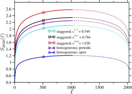
Figure 1: Entropy of finite chains of length $L=2048$ vs subsystem size $\ell$: the full curves for $\ell\leq L/2$ are calculated numerically; the dashed curves for $\ell\geq L/2$ are the corresponding conformal results, described by Eq. (2) with $c=1/2$ and $c_{1}=0.690413$ for homogeneous chains with periodic boundary conditions, and by Eq. (3) with $g=1$ for open homogeneous chains. For chains with staggered interactions, there are four branches, depending on the type of the couplings on the boundary of the subchain. Data presented here are for staggered chains with $\lambda=0.5$ and with periodic boundary conditions. The fits for $\ell\geq L/2$ using Eq. (2) are fulfilled with $c=1/2$, $c_{1}^{(++)}=1.02009$ (two strong couplings on the boundary), $c_{1}^{(+-)}=c_{1}^{(-+)}=0.78446$ (one strong and one weak coupling) and $c_{1}^{(--)}=0.54883$ (two weak couplings), respectively.

Furthermore, we are interested in the finite-size correction terms for the coefficient $c$ and the boundary entropy $\log_{2}g$ given in Eq. (3). To evaluate $c$ for different system size, we first calculate the entropy difference $\Delta S(L)=S_{L}(L/2)-S_{L/2}(L/4)$. For a chain with periodic boundary conditions, we have $\Delta S(L)=c(L)/3$ and obtain an $L^{-2}$ - correction for the coefficient: $c(L)=0.5-0.623(1)/L^{2}+O(L^{-3})$; for an open chain, we obtain a $L^{-1}$ - correction, $c(L)=0.5+1.339(1)/L+O(L^{-2})$, via $\Delta S(L)=c(L)/6$. To compute the boundary entropy $g(L)$, we make use the relation between $S_{L}^{(p)}$ and $S_{L}^{(o)}$ for periodic and open boundary conditions, respectively, via $2S_{L}^{(o)}(\ell)-S_{L}^{(p)}(\ell)=\log_{2}g(L)+c/3$. In Table 1, the values of $g(L)$ using $\ell=L/2$ and $c=1/2$ are given for system sizes up to $L=4096$, and it shows a correction of $O(1/L)$.

In conclusion, our numerical results for the entanglement entropy of the homogeneous quantum Ising chain agree with all the known conformal predictions.

3.2 Chains with staggered interactions

Now we consider the quantum Ising chain with periodically varying interactions of period 2, corresponding to a chain with staggered interactions: $J_{2i-1}=\lambda$ and $J_{2i}=1/\lambda$. According to Eq. (12), the critical point of the system is located at $h_{c}=1$. This quantum Ising chain with staggered interactions has been solved in Ref. [33], and its critical singularities were found to be the same as for the homogeneous chain. Here we study the entanglement entropy of the staggered chain and check its relationship with the entropy of the homogeneous chain.

First, we calculate the entanglement entropy, $S_{L}(\ell)$, as a function of the subsystem size $\ell$, for a finite chain. As shown in Fig. 1 for a chain of length $L=2048$ with $\lambda=0.5$, there are four branches with a twofold degeneracy, depending on the type of the couplings ($\lambda$ or $\lambda^{-1}$) at the boundaries of the subsystem. For each $\ell$, the largest and smallest value of $S_{L}(\ell)$ correspond to the case in which both boundary couplings are strong (denoted by $(++)$) and weak ($(--)$), respectively, and the twofold degeneracy lying in between occurs when one boundary coupling is strong and one weak ($(+-)$ and $(-+)$). All branches are well fitted by the conformal form in Eq. (2) with coefficient $c=1/2$ corresponding to the central charge of the homogeneous case, but with different additive constants $c_{1}$. The additive constants for the above mentioned four branches satisfy the relation: $c_{1}^{(++)}+c_{1}^{(--)}=2c_{1}^{(+-)}$. This means that the boundary effect is strictly additive: $c_{1}^{(++)}=2c_{1}^{(+)}$, $c_{1}^{(+-)}=c_{1}^{(+)}+c_{1}^{(-)}$ and $c_{1}^{(--)}=2c_{1}^{(-)}$, here the subscript $+$ ($-$) corresponds to one strong (weak) boundary coupling. For $\lambda=0.5$ we have $c_{1}^{(+)}=0.510045$ and $c_{1}^{(-)}=0.274415$, whereas for $\lambda=0.25$ these are $c_{1}^{(+)}=0.663435$ and $c_{1}^{(-)}=0.262845$. Furthermore, $c_{1}^{(+)}$ ($c_{1}^{(-)}$) is found to be a monotonously increasing (decreasing) function of $1/\lambda\geq 1$, and the average, $c_{1}^{(+-)}/2$, is minimal for the homogeneous chain $\lambda=1$. Consequently, for irrelevant perturbations represented by the staggered interaction the average critical entanglement entropy is increasing, compared with the fixed point value of the homogeneous chain.

To see how the coefficient $c(L)$ for a finite chain of length $L$ approaches the conformal value $c=1/2$, we follow the procedure described in Sec. 3.1 for the homogeneous chain. Like the homogeneous chain, the leading term of the finite-size correction to $c(L)$ is found to be $O(L^{-2})$ for periodic boundary conditions, and $O(L^{-1})$ for open boundary conditions.

3.3 Random chains

The entanglement entropy of the quantum Ising model with random couplings and/or transverse fields can be conveniently studied by the strong disorder renormalization group (RG) method[8, 21]. In this RG representation, the ground state of the quantum Ising model consists of a collection of independent ferromagnetic clusters of various sizes; each cluster of $n$ spins is in a $n$-site entangled state $\frac{1}{\sqrt{2}}(\left|\uparrow\right\rangle^{\otimes n}+\left|\downarrow\right\rangle^{\otimes n})$. The entanglement entropy of a subsystem is just given by the number of the clusters that cross the boundary of the subsystem. In 1D the asymptotic number of such clusters that contribute to the entropy of a subsystem of length $\ell$ has been analytically calculated by Refael and Moore [8] and the disorder average entropy in the long chain limit is found to scale as:

$$\overline{S}(\ell)=\frac{c_{\rm eff}}{3}\log_{2}\ell+c_{1}^{\prime}$$ (23)

where the effective central charge, $c_{\rm eff}=\ln 2/2$, is expected to be universal, i.e. does not depend on the form of disorder, whereas the additive constant, $c_{1}^{\prime}$, is disorder dependent.

For a finite chain of length $L$ with periodic boundary conditions, the entropy of a subsystem of length $\ell$ is expected to behave as:

$$\overline{S}_{L}(\ell)=\frac{c_{\rm eff}}{3}\log_{2}[Lf(\ell/L)]+c_{1}^{\prime}$$ (24)

where the scaling function $f(v)$ is reflection symmetric, $f(v)=f(1-v)$, and $\lim_{v\to 0}f(v)\simeq v$. Consequently $f(v)$ can be expanded as a Fourier series: $f(v)=\sum_{k=1}^{\infty}A_{k}\sin(2k-1)\pi v$, with $\sum_{k=1}^{\infty}A_{k}(2k-1)\pi=1$. We note that for conformally invariant models only the first term of this expansion exists (cf. Eq. (2)).

In our numerical calculations we used a power-law distribution:

$$P_{D}(x)=\frac{1}{D}x^{-1+1/D}\;,$$ (25)

both for the couplings and the transverse fields, which ensures that the random model is at the critical point. Here $D^{2}=\overline{\ln^{2}x}-\overline{\ln x}^{2}$ measures the strength of disorder. For the random chains we have treated finite chains up to a length $L=1024$, and considered at least $10^{4}$ independent realizations for each length $L$, plus different positions of a subsystem in the chain for a given $\ell$.

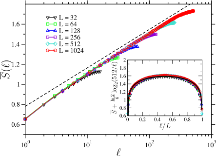
Figure 2: Average entropy of the random chain with uniform disorder (with $D=1$) as a function of $\ln\ell$ for different system sizes $L$. The slope of the broken straight line is given by $1/6$, corresponding to the RG prediction $c_{\rm eff}=\ln 2/2$. Inset: scaling plot of the entropy vs. $\ell$ for different sizes $L$ using the scaling prediction in Eq. (24). The solid line corresponds to the conjecture of conformal invariance, given in Eq. (2), with $c$ replaced by $c_{\rm eff}=\ln(2)/2$ and an additive constant as the fit parameter.

In Fig. 2 we plot the average entropy $\overline{S}_{L}(\ell)$ vs. $\ln\ell$. The curves tend to approach an asymptotic linear behavior with a slope which is, in the large $\ell$ regime, well described by the renormalization group prediction $c_{\rm{eff}}=\ln(2)/2$. To estimate $c_{\rm eff}(L)$ quantitatively for different chain sizes $L$, we average over the entropy in the large $\ell$ region and make use of the relation between $\overline{S}_{2L}$ and $\overline{S}_{L}$, given by

$$\frac{1}{2n+1}\sum_{\ell=L/2-n}^{L/2+n}[\overline{S}_{2L}(2l)-\overline{S}_{L}(l)]=c_{\rm eff}(2L)/3.$$ (26)

The estimated values of $c_{\rm eff}(L)/\ln 2$ are presented in Table 2 for uniform disorder. The results for the two largest finite systems are compatible with the estimate: $c_{\rm eff}/\ln 2=0.501(3)$, which is in excellent agreement with the RG prediction.

Table 2: Finite-size estimates of $c_{\rm eff}/\ln 2$ for the random model using the relation in Eq.(26).

• n	$L=128$	$L=256$	$L=512$
  2	0.531	0.503	0.502
  4	0.532	0.502	0.506
  8	0.533	0.502	0.501
  16	0.534	0.504	0.499

Finally we turn to a study of the form of the average entropy $\overline{S}_{L}(\ell)$ as a function of $\ell$, in particular we are interested in how well it can be approximated by the conjecture of conformal invariance given in Eq. (2) with an effective central charge $c_{\rm{eff}}$. As shown in the inset of Fig. 2, the approximation is seemingly good. To have a quantitative comparison, we have calculated the ratio $\overline{r}(L)$, similar to Eq. (22), defined as

$$\overline{r}(L)=\frac{\overline{S}_{L}(L/2)-\overline{S}_{L}(L/4)}{\overline{S}_{2L}(L)-\overline{S}_{L}(L/2)},$$ (27)

whose asymptotic value is given, in terms of the Fourier coefficients, by:

$$\overline{r} = \frac{1}{2}+\log_{2}\left[\sum_{k=1}^{\infty}(-1)^{k+1}A_{k}\right]$$ (28)

$$- \log_{2}\left[\sum_{k=1}^{\infty}(-1)^{k+1}(A_{2k-1}+A_{2k})\right]\;.$$ (29)

For conformal invariant cases, we have $\overline{r}=1/2$. The numerically calculated values of $\overline{r}(L)$, presented in Table 3 for disorder strength $D=0.5$ and $D=1$, deviate significantly from $\overline{r}=1/2$ for large $L$. This means that the higher order terms in the Fourier expansion are not negligible. The scaling function $f(v)$ is presumably universal, i.e. independent of the form of the disorder.

Table 3: The ratio defined in Eq. (27) for the average entropy $\overline{S}_{L}(\ell)$ for disorder strength $D=0.5$ and $D=1$.

• L	$D=0.5$	$D=1.0$
  32	0.548	0.587
  64	0.588	0.605
  128	0.573	0.584
  256	0.619	0.608
  512	0.615	0.606

4 Scaling close to the critical point

So far we have studied the entanglement entropy at the critical point. In this section, we consider the entanglement between two halves of a finite chain with homogeneous interactions, and study its behavior approaching to the critical point $h_{c}=1$.

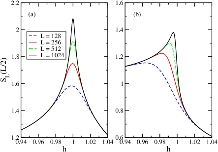
Figure 3: The entanglement entropy of a half of a chain with $J=1$ as a function of the strength of the transverse field $h$, for periodic (a) and open (b) boundary conditions. On increasing the system size $L$, the maximum gets more pronounced, and the position of the maximum tends towards the critical point $h_{c}=1$.

According to Eq. (4) and Eq. (5), a divergence of the maximal entanglement entropy occurs at the quantum critical point, which can be traced back to the divergence of the correlation length with $\xi\sim|h-h_{c}|^{-\nu}$. In a finite system of length $L$, the finite size effects induce a rounding and a shift of the maximum of the entropy, as shown in Fig. 3 for $S_{L}(L/2)$ vs. $h$. In the following we denote the entropy of a half of a finite chain of length $L$ as a function of the transverse field $h$ by $S_{L}(L/2,h)\equiv\hat{\cal S}(L,h)$. The position of the maximum of $\hat{\cal S}(L,h)$, denoted by $h_{m}(L)$, can be used to define a finite-size effective critical point and its shift from the true critical point is expected to scale as: $h_{c}-h_{m}(L)\sim L^{-\lambda}$, where $\lambda$ is the shift exponent. The numerically calculated finite-size transition points are listed in Table 4 both for closed and open chains. The maximum of the entropy $\hat{\cal S}(L,h_{m}(L))$, like $\hat{\cal S}(L,h_{c})$, depends logarithmically on the system sizes $L$ [insets in Fig. 4 and Fig. 5]. As a matter of fact the difference $\Delta S(L)=\hat{\cal S}(L,h_{m}(L))-\hat{\cal S}(L,h_{c})$ approaches a well defined limiting value for $L\to\infty$. Note, however that for open chains $\Delta S(L)$ tends to a finite value, whereas for closed chains the entropy difference goes to zero.

We first study the rounding of the maximum of the entropy. Making use of the finite-size scaling ansatz[34]:

$$\hat{\cal S}(L,h)-\hat{\cal S}(L,h_{m}(L))=\widetilde{F}[L^{1/\nu}(h-h_{m}(L))]\;.$$ (30)

with $\nu=1$, we can make all data for different system sizes perfectly collapse onto a single curve, as shown in Fig. 4 for open chains and Fig. 5 for closed chains. In both cases the scaling function is $\widetilde{F}[\tilde{x}]\sim\tilde{x}^{2}$ for small $\tilde{x}$.

In order to obtain the shift of the finite-size critical points, we take the derivative of both sides of Eq.(30) at $h=h_{c}$:

$$\left.\frac{\partial\hat{\cal S}(L,h)}{\partial h}\right|_{h_{c}}\sim L^{2/\nu}(h_{c}-h_{m}(L))\;.$$ (31)

For open chains the derivative at the l.h.s. is proportional to $L^{1/\nu}$, leading to conventional finite-size scaling relation: $h_{c}-h_{m}(L)\sim L^{-1/\nu}$. For closed chains this derivative has a much weaker $L$-dependence, which can be identified as logarithmic in $L$. From Eq. (31), we then expect the relation: $h_{c}-h_{m}(L)\sim\log_{2}L/L^{2}$. This prediction can be checked by calculating the shift exponent $\lambda$ through the finite-size estimates: $\lambda(L)=\log_{2}[h_{c}-h_{m}(L/2)]-\log_{2}[h_{c}-h_{m}(L)]$ [Table 4]. For open chains the exponent approaches $\lambda=1/\nu=1$ for large $L$, in accordance with our previous discussion. For closed chains the effective shift exponent is around $1.87$ for the largest system size, which, however, cannot rule out a true value $\lambda=2$ with a logarithmic finite-size-correction. In B we present an argument in favor of the $\log_{2}L/L^{2}$ behavior of the shift for closed chains. As a numerical check of this scenario we have calculated the scaling combination: $sc=(1-h_{m}(L))\times L^{2}/(\log_{2}L+a)$, which are shown in Table 4. Indeed the value of $sc$ seems to approach a finite limiting value.

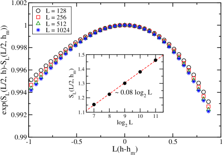
Figure 4: A scaling plot of the entanglement entropy for chains with open boundary conditions. Data collapse is obtained for $\nu=1$, consistent with the universality hypothesis. In the inset is shown the divergence of the value at the maximum as the system size increases. The slope is given by 0.08, consistent with the exact value $1/12$ (cf. Eq. (5)).

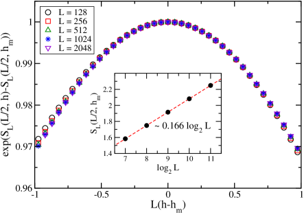
Figure 5: The finite size scaling is performed for chains with periodic boundary conditions, using the scaling form in Eq. (30) and $\nu=1$. The inset shows the logarithmic dependence of the value at the maximum on the system size $L$. The slope is consistent with the theoretical value $1/6$ for a half subchain taken from a closed chain.

Having clarified the finite-size scaling behavior of the rounding and the shift of the maximum of the entropy, let us consider the scaling form of the entropy in the critical region. In the conventional finite-size scaling theory we have the ansatz:

$$\hat{\cal S}(L,h)-\hat{\cal S}(L,h_{c})=F[L^{1/\nu}(h-h_{c})]\;.$$ (32)

The l.h.s. of Eq.(32) can be rewritten as: $\hat{\cal S}(L,h)-\hat{\cal S}(L,h_{m}(L))+\Delta S(L)=\widetilde{F}[\tilde{x}]+\Delta S(L)$, where the argument of $\widetilde{F}(\tilde{x})$ is given by: $\tilde{x}=x-x_{c}$ with $x=L^{1/\nu}(h-h_{c})$ and $x_{c}=L^{1/\nu}(h_{c}-h_{m}(L))$. Now using the fact that $\widetilde{F}[\tilde{x}]$ is quadratic for small $\tilde{x}$ we obtain for the scaling function in Eq.(32):

$$F(x)\approx A(x-x_{c})^{2}+\Delta S,\quad x\approx x_{c}\;.$$ (33)

For open chains in the large $L$ limit, we have $x_{c}>0$ and $\Delta S>0$, so that shift exponent is $\lambda=1/\nu$. On the other hand, for closed chains both limiting values vanish: $x_{c}=0$ and $\Delta S=0$. Therefore conventional finite-size scaling is not valid and the shift exponent is $\lambda>1/\nu$.

We close this section by two remarks. First we note that in Ref [1] the derivatives of the nearest-neighbor concurrence, $\partial_{J}C(1)$, with respect to the control parameter $J$ is studied. The position of the minimum of $\partial_{J}C(1)$, which defines the effective quantum critical point of a finite closed chain of length $L$, is shifted from the true critical point by $L^{-1.87}$ (see Fig. 1, in Ref. [1]), with a shift exponent that is very close to the effective exponent given in Table 4. One might think that the shift of the minimum of $\partial_{J}C(1)$ has the same scaling behavior as discussed here for the position of the maximum of the entropy.

Our second remark concerns random chains. The position of the maximum of the average entanglement entropy of a half chain can be used to define sample dependent pseudocritical point. Its scaling has been studied in detail in Ref. [29].

Table 4: Finite-size critical transverse fields of the homogeneous quantum Ising chain of $L$ sites with periodic [p] and open [o] boundary conditions calculated from the location of the maxima of the entropy for $\ell=L/2$. The effective shift exponents, $\lambda(L)$, are calculated by two point fits. The scaling combinations are: $sc=(1-h_{m}(L))\times L^{2}/(\log_{2}L+a)$ with $a=2-1/\ln 2$ (s. Appendix B), for periodic chains and $x_{c}=(1-h_{m}(L))\times L$ for open chains.

• L	$h_{m}(L)[p]$	$\lambda(L)$	$sc$	$h_{m}(L)[o]$	$\lambda(L)$	$x_{c}$
  128	0.9983031	1.813	3.679	0.9636656	1.077	4.651
  256	0.9995225	1.829	3.656	0.9822266	1.045	4.550
  512	0.9998671	1.845	3.644	0.9912353	1.027	4.487
  1024	0.9999633	1.858	3.641	0.9956543	1.015	4.450
  2048	0.9999900	1.876	3.629	0.9978379	1.007	4.424

5 Discussion

In this paper we have studied finite size effects of entanglement entropy of the quantum Ising chain at/near its order-disorder quantum phase transition. The model considered can be expressed in terms of free fermions, which enables us to perform large scale numerical investigations. Three types of couplings were considered: homogeneous, periodically modulated and random couplings.

For the homogeneous system at the critical point we have verified the finite size form predicted by the conformal field theory, both for periodic and open boundary conditions. We have also calculated the additive constant to the entropy and subleading corrections. In the off-critical region, we have studied the finite-size scaling behavior of the entropy, $S_{L}(L/2)$, in the vicinity of its maximum, and confirmed the intimate connection between entanglement and universality. The position of the maximum, $h_{m}(L)$, can be regarded as an indicator of the effective critical point in the finite sample. For an open chain the shift of $h_{m}(L)$ from the true critical point is shown to be $O(L^{-1})$, whereas for a chain with periodic boundary conditions it is $O(L^{-2}\ln L)$. We have provided analytical results for the off-critical entropy in infinite chains to explain these findings. We expect that the shift of $h_{m}(L)$ for other critical quantum spin chain has the same type differences for open and periodic boundary conditions.

The quantum Ising chain with periodically modulated couplings belongs to the same critical universality class as the homogeneous model. In the case of staggered couplings, we have found that the critical entropy is split into four branches, each of which has the same prefactor (the central charge) of the logarithm but has different additive constants. This is expected to be generic to critical quantum spin chains with all kinds of periodically modulated couplings.

For random quantum Ising chains, we have numerically verified the prefactor of the logarithm predicted by the analysis of the strong disorder renormalization group. The functional form of the average entropy versus subsystem size, which is presumably universal for any strength of disorder, has been found to deviate from the results for conformally invariant models.

The results obtained in this paper, though only based on quantum Ising chains, are expected to be valid in some other cases of quantum spin chains. For example, the XY-chain is related with the Ising chain via an exact mapping, so that the results obtained for the Ising chain can be directly transferred to those for the XY-chain through the mapping. This mapping is also applicable for random cases. Moreover, for random cases the criticality of many quantum spin chains belongs to the same universality class (cf. random XX-chains and random Heisenberg chains), known from the strong-disorder renormalization group, and the universality of the associated effective central charge was numerically confirmed [35]. Therefore, our results for the random cases, e.g. the functional form of the average entropy vs. $\ell$, should be universal for a wide range of models.

Appendix A The correlation matrix for homogeneous chains

For the critical homogeneous chain the free-fermion transformation can be performed analytically, both for closed and for open finite chains. In the following we consider the case where the length of the chain $L$ is even.

A.1 Closed chain

For a closed chain with $J_{L}=J=1$ and $h=1$ the positive eigenvalues of Eq.(11) are two-fold degenerate, which are given by:

$$\Lambda_{k}=2\sin\left[\frac{2k-1}{L}\frac{\pi}{2}\right]\;,$$ (34)

for $k=1,2,\dots,L/2$. One set of the eigenvectors is:

$$\phi^{(1)}_{k}(j) = (-1)^{j}\sqrt{\frac{2}{L}}\sin\left[\frac{2k-1}{L}\left(j-1/2\right)\pi\right]$$ (35)

$$\psi^{(1)}_{k}(j) = (-1)^{j}\sqrt{\frac{2}{L}}\cos\left[\frac{2k-1}{L}j\pi\right]\;,$$ (36)

and the second set is:

$$\phi^{(2)}_{k}(j) = (-1)^{j+1}\sqrt{\frac{2}{L}}\cos\left[\frac{2k-1}{L}\left(j-1/2\right)\pi\right]$$ (37)

$$\psi^{(2)}_{k}(j) = (-1)^{j}\sqrt{\frac{2}{L}}\sin\left[\frac{2k-1}{L}j\pi\right]\;,$$ (38)

Then the reduced correlation matrix is given by:

$$G_{m,n}=\frac{(-1)^{m-n}}{L\sin\left(\frac{\pi}{2L}[2(m-n)+1]\right)}.$$ (39)

A.2 Open chain

For open chains with $J_{L}=0$ the solution at the critical point reads:

$$\phi_{k}(j) = (-1)^{j}\frac{2}{\sqrt{2L+1}}\cos\left[\frac{2k-1}{2L+1}\left(j-1/2\right)\pi\right]$$ (40)

$$\psi_{k}(j) = (-1)^{j+1}\frac{2}{\sqrt{2L+1}}\sin\left[\frac{2k-1}{2L+1}j\pi\right]\;,$$ (41)

and the energy of the free-fermionic modes are given by:

$$\Lambda_{k}=2\sin\left[\frac{2k-1}{2L+1}\frac{\pi}{2}\right]\;.$$ (42)

for $k=1,2,\dots L$. The reduced correlation matrix reads:

$$G_{m,n}=\frac{(-1)^{m+n}}{L+1/2}\left\{\frac{\sin^{2}(\beta_{m,n}^{-}L)}{\sin(\beta_{m,n}^{-})}+\frac{\sin^{2}(\beta_{m,n}^{+}L)}{\sin(\beta_{m,n}^{+})}\right\}$$ (43)

with $\beta_{m,n}^{\pm}=\pi[m\pm(n-1/2)]/(2L+1)$.

A.3 Infinite chain limit

In the infinite system limit, $L\to\infty$, $n/L=O(1)$, $m/L=O(1)$ and $m-n\leq\ell$ for both boundary conditions we recover the known result[26, 27]:

$$G_{m,n}=\frac{2}{\pi}\frac{(-1)^{m-n}}{2(m-n)+1}\;.$$ (44)

Appendix B The shift exponent for closed chains

To explain the finite-size scaling behavior of $\hat{\cal S}(L,h)$ for closed chains, we recall the entropy in the infinite system analytically obtained in Ref. [15, 16]. Here we write it in terms of the variable, $\gamma=(1-h)/(1+h)$, as:

$$S = \frac{1}{12}\left\{\log_{2}\left[\frac{4(1-\gamma)^{4}}{(1+\gamma)^{2}|\gamma|}\right]\right.$$ (45)

$$+ \left.\frac{2}{\pi\ln 2}(1+6\gamma+\gamma^{2})I(\gamma)I(\gamma^{\prime})\right\},$$ (46)

where $I(\gamma)$ denotes the complete elliptic integral of the first kind and $\gamma^{\prime}=\sqrt{1-\gamma^{2}}$. The advantage of the form given in Eq. (46) is that it is valid both for $h<1$ and $h>1$.

We note that the entropy is not symmetric with respect to $h_{c}=1$; if we compare its value at $h$ and $h^{-1}$, it is larger in the ordered phase, $h<1$, by an amount of $\Delta S(h)=S(h)-S(h^{-1})$:

$$\Delta S(h) = \frac{1}{2}\left[\log_{2}\frac{1-\gamma}{1+\gamma}+\frac{4}{\pi\ln 2}I(\gamma)I(\gamma^{\prime})\right]$$ (47)

$$\underset{\gamma\ll 1}{\rightarrow} \gamma\left[-\log_{2}\gamma+2-\frac{1}{\ln 2}\right].$$ (48)

The last equation for small $\gamma$ is valid in the vicinity of the critical point. Next we define for each $h<1$ a transverse field $h^{\prime}>1$ via the relation: $S(h)=S(h^{\prime})$. Close to the critical point the distance between $h^{-1}$ and $h^{\prime}$ is given by:

$$\Delta h=h^{-1}-h^{\prime}\approx\frac{\Delta S(h)}{\partial S/\partial h}\approx\gamma^{2}\left[-\log_{2}\gamma+2-\frac{1}{\ln 2}\right].$$ (49)

which vanishes only at the critical point. Now let us consider a large finite system of length $L$ at the transverse field $h=h(L)$, where the singularity of the entropy starts to be rounded (this happens when $[\hat{\cal S}(L,h)-\hat{\cal S}(\infty,h)]/\hat{\cal S}(\infty,h)$ exceeds some small limiting value). For closed chains, in which there are the same number of couplings and transverse fields, the same is true at the corresponding point, $h^{\prime}(L)$, too. The position of the maximum of $\hat{\cal S}(L,h)$ is about at $h_{m}(L)\approx[h(L)+h^{\prime}(L)]/2$. If the entropy is symmetric at $h$ and $h^{-1}$, the estimate of the transition point would be: $h_{c}^{\rm{sym}}(L)\approx[h(L)+h^{-1}(L)]/2$, and the distance between $h_{m}(L)$ and $h_{c}^{\rm{sym}}(L)$ is about $\sim\Delta h(L)/2$. This value is in the same order as the shift of the finite-size transition point. Making use of the fact that $L\sim\xi\sim\gamma^{-1}$, we obtain from Eq.(49)

$$\Delta h(L)\sim(h_{c}-h_{m}(L))\sim L^{-2}\left[\log_{2}L+a\right]$$ (50)

with $a\approx 2-1/\ln 2$. This means that the true value of the shift exponent is $\lambda=2$, but there is a strong logarithmic correction, which makes the numerical calculation of $\lambda$ very difficult.

References

References

- [1] A. Osterloh, L. Amico, G. Falci, and R. Fazio, Nature 416, 608 (2002).
- [2] T. J Osborne and M. A. Nielsen, Phys. Rev. A 66, 032110 (2002).
- [3] For a review, see: L. Amico, R. Fazio, A. Osterloh and V. Vedral, Rev. Mod. Phys. 80, 517 (2008).
- [4] M. Srednicki, Phys. Rev. Lett. 71, 666 (1993).
- [5] G. Vidal, J. I. Latorre, E. Rico, and A. Kitaev, Phys. Rev. Lett. 90, 227902 (2003); J. I. Latorre, E. Rico, and G. Vidal, Quantum Inf. Comput. 4, 048 (2004).
- [6] C. Holzhey, F. Larsen, and F. Wilczek, Nucl. Phys. B 424 44 (1994); V. E. Korepin, Phys. Rev. Lett. 92 096402 (2004).
- [7] P. Calabrese and J. Cardy, J. Stat. Mech. P06002 (2004).
- [8] G. Refael and J. E. Moore, Phys. Rev. Lett. 93, 260602 (2004).
- [9] M.M. Wolf, Phys. Rev. Lett. 96, 010404 (2006); D. Gioev and I. Klich, Phys. Rev. Lett. 96, 100503 (2006); S. Farkas and Z. Zimborás, J. Math. Phys. 48, 102110 (2007).
- [10] T. Barthel, M.-C. Chung, and U. Schollwöck, Phys. Rev. A 74, 022329 (2006).
- [11] M. Cramer, J. Eisert, and M.B. Plenio, Phys. Rev. Lett. 98, 220603 (2007).
- [12] Y.-C. Lin, F. Iglói and H. Rieger, Phys. Rev. Lett. 99, 147202 (2007).
- [13] R. Yu, H. Saleur and S. Haas, Phys. Rev. B 77, 140402 (2008).
- [14] I. Affleck and A.W.W. Ludwig, Phys. Rev. Lett. 67, 161 (1991).
- [15] I. Peschel, J. Stat. Mech. P12005 (2004).
- [16] B.-Q. Jin and V.E. Korepin, J. Stat. Phys. 116, 79 (2004); A. R. Its, B.-Q. Jin and V.E. Korepin, Fields Institute Communications, Universality and Renormalization [editors I.Bender and D. Kreimer] 50, 151 (2007).
- [17] H.-Q. Zhou, Th. Barthel, J.O. Fraerestad, and U. Schollwöck, Phys. Rev. A74, 050305(R) (2006).
- [18] F. Iglói and R. Juhász, Europhys. Lett. 81, 57003 (2008).
- [19] S.-K. Ma, C. Dasgupta, and C.-K. Hu, Phys. Rev. Lett. 43, 1434 (1979).
- [20] D.S. Fisher, Phys. Rev. Lett. 69, 534 (1992); Phys. Rev. B 51, 6411 (1995).
- [21] For a review, see: F. Iglói and C. Monthus, Physics Reports 412, 277, (2005).
- [22] R. Santachiara, J. Stat. Mech. Theor. Exp. L06002 (2006).
- [23] N.E. Bonesteel and Kun Yang, Phys. Rev. Lett. 99, 140405 (2007).
- [24] G. Refael and J. E. Moore, Phys. Rev. B 76, 024419 (2007).
- [25] F. Iglói, R. Juhász and Z. Zimborás, Europhys. Lett. 79, 37001 (2007); R. Juhász and Z. Zimborás, J. Stat. Mech. Theor. Exp. 2007, P04004 (2007).
- [26] E. Lieb, T. Schultz and D. Mattis, Annals of Phys. 16, 407 (1961).
- [27] P. Pfeuty, Phys. Lett. 72A, 245 (1979).
- [28] F. Iglói and l. Turban, Phys. Rev. Lett. 77, 1206 (1996); F. Iglói, L. Turban, D. Karevski and F. Szalma, Phys. Rev. B56, 11031 (1997).
- [29] F. Iglói, Y.-C. Lin, H. Rieger and C. Monthus, Phys. Rev. B 76, 064421 (2007).
- [30] I. Peschel, J. Phys. A: Math. Gen. 36, L205 (2003).
- [31] J. Cardy, Nucl. Phys. B 324, 581 (1989); J. Cardy and D. Lewellen, Phys. Lett. B 259, 274 (1991).
- [32] J. L. Cardy, O. A. Castro-Alvaredo and B. Doyon, J. Stat. Phys. 130, 129 (2007).
- [33] F. Iglói and J. Zittartz, Z. Physik B70, 387 (1988).
- [34] M. N. Barber, Phase Transitions and Critical Phenomena Vol. 8 [eds. C. Domb and J. L. Lebowitz] 146 (Academic Press, London, 1983).
- [35] N. Laflorencie, Phys. Rev. B 72, 140408(R) (2005); G. De Chiara, S. Montangero, P. Calabrese and R. Fazio, J. Stat. Mech. P03001 (2006).